Hybrid Spatio-Temporal CNN–LSTM/BiLSTM Models for Blocking Prediction in Elastic Optical Networks

Abstract

Elastic optical networks (EONs) must allocate resources dynamically to accommodate heterogeneous, high-bandwidth demands. However, the continuous setup and teardown of connections with different bit rates can fragment the spectrum and lead to blocking. The blocking predictors enable proactive defragmentation and resource reallocation within network controllers. In this paper, we propose two novel deep learning models (based on CNN–BiLSTM and CNN–LSTM) to predict blocking in EONs by combining spatial feature extraction from spectrum snapshots using 2D convolutional layers with temporal sequence modeling. This hybrid spatio-temporal design learns how local fragmentation patterns evolve over time, allowing it to detect impending blocking scenarios more accurately than conventional methods. We evaluate our model on the simulated NSFNET topology and compare it against multiple baselines, namely 1D CNN, 2D CNN, k-nearest neighbors (KNN), and support vector machines (SVMs). The results show that the proposed CNN–BiLSTM/LSTM models consistently achieve higher performance. The CNN–BiLSTM model achieved the highest accuracy in blocking prediction, while the CNN–LSTM model shows slightly lower accuracy; however, it has much lower complexity and a faster learning time.

1. Introduction

Services that require high bandwidth, such as ultra-high-definition video streaming, cloud gaming, telepresence, and virtual reality, are increasing the need for fast optical networks. Traditional optical networks use fixed-grid Wavelength Division Multiplexing (WDM), usually with channel widths of 50 or 100 GHz. This method often leads to unused spectrum when the bandwidth requested is smaller than the channel size, particularly when different types of traffic are combined.

EONs were developed to overcome the limitations of traditional optical networks. They divide large frequency bands into smaller frequency slots, such as 12.5 GHz or 6.25 GHz, which can be combined flexibly according to the bandwidth needed for each connection. By allowing dynamic spectrum allocation, EONs offer a more flexible and cost-effective way to handle the growing network and internet traffic demands [1].

However, the flexibility of EONs can also result in spectrum fragmentation. When connections are repeatedly set up and terminated, available frequency slots can become scattered. As a result, even if there is a large total amount of free spectrum, it may not contain enough continuous slots to accommodate new connection requests [2]. Spectrum fragmentation increases the likelihood of rejecting new connections, which in turn increases connection blocking probability and reduces the overall efficiency of the network [3]. Although many metrics have been proposed to represent fragmentation [4], its impact on blocking probability is difficult to quantify. Therefore, using a comprehensive view of the spectral status of links, as proposed in this work, can be valuable in mitigating the effects of fragmentation.

The issue of spectrum fragmentation can be addressed by performing spectrum defragmentation or rerouting to restore contiguous frequency slots [5]. However, repeated execution of these actions may lead to unnecessary resource consumption, while delaying them could result in blocked connections [6,7]. Therefore, it is important to correctly predict when the risk of blocking increases and intervene at the appropriate time [8].

Predicting network blocking events is a critical challenge. Deep learning techniques can provide powerful predictive capabilities to optimize performance and enhance network reliability. Early machine learning attempts modeled blocking as a classification problem fed with specifically designed traffic features or spectrum occupancy statistics [9,10,11,12].

Blocking prediction has been an important topic in recent research in EONs. Singh and Jukan [13] proposed a reduced-state Markov model for blocking probability estimation in EONs. Moreover, analytical traffic models such as Erlang B have been evaluated for their applicability in EONs. Ujjwal and Thangaraj [14] investigated the limitations of Erlang B in estimating blocking probability under dynamic RSA scenarios. Cheng and Qiu [15] introduced a Long Short-Term Memory (LSTM)-based routing and spectrum assignment (RSA) framework, which learns temporal network dynamics to anticipate spectrum usage and predict blocking trends. Dávalos et al. [16] proposed a machine learning-based triggering strategy for spectrum defragmentation in EONs. Their method estimates the blocking rate using neural networks and activates defragmentation only when necessary, outperforming fixed-time and metric-based triggering approaches by reducing both blocking demands and unnecessary reconfigurations.

The authors in [1] demonstrated that two-dimensional Convolutional Neural Networks (2D-CNNs) trained directly on spectrum status matrices can reach an accuracy of 92.17% in blocking prediction on EONs based on the NSFNET topology, significantly outperforming support vector machines and k-Nearest Neighbors baselines.

Recent works on routing, spectrum assignment, and traffic forecasting indicate that combining spatial convolutions with recurrent units able to model time series yields superior results in optical networks [17]. Current blocking predictors either neglect the temporal dynamics of fragmentation or rely on handcrafted features that fail to generalize across topologies and traffic patterns. As a consequence, network operators still lack actionable and timely alarms that would allow them to schedule defragmentation exactly when it is needed.

Traffic prediction and dynamic resource management in EONs have gained substantial attention with the advent of machine learning (ML) techniques [18,19]. Deep reinforcement learning (DRL) methods have particularly emerged as powerful tools for routing and spectrum assignment (RSA) challenges [20,21]. Panayiotou et al. [17] propose a DRL-based RSA solution leveraging Graph Convolutional Networks (GCNs) for topological feature extraction and Recurrent Neural Networks (RNNs) for aggregating path-level features, addressing the limitations of Conventional Neural Networks (CNNs) in capturing network topology.

The broader survey by Panayiotou et al. [17] discusses the role of CNNs and Long Short-Term Memory (LSTM) networks in traffic prediction for wireless networks, emphasizing their capacity to model spatial and temporal dependencies, respectively. Deep Convolutional Recurrent Neural Networks (DCRNNs) effectively capture spatio-temporal traffic patterns, outperforming traditional methods [22].

Azzouni and Pujolle [23] introduced NeuTM, an LSTM-based framework for predicting traffic matrices in Software-Defined Networks (SDNs), demonstrating low mean square error performance on the GÉANT backbone. For EON-based cloud networks, Monte Carlo Tree Search (MCTS) and artificial neural network (ANN) approaches were evaluated by Aibin and Walkowiak [24] to predict load and minimize blocking. Similarly, Poupart et al. [25] predicted flow sizes to proactively manage routing decisions, while Nie et al. [26] applied Deep Belief Networks (DBNs) to predict traffic in wireless mesh backbones, decomposing traffic dynamics into predictable and irregular components. Most of the high-speed wireless networks, such as 4G and 5G, use EONs as a backbone.

Fault detection and resilience in EONs have also benefited from ML integration. Reddy and Kumar [27] proposed a deep neural network (DNN) combined with a Fuzzy Inference System (FIS) to enhance Shared Backup Path Protection (SBPP), improving the fault restoration ratio while reducing blocking probabilities. Multi-step traffic forecasting has been shown to outperform single-step predictions. Maryam et al. [28] utilized an Encoder–Decoder LSTM (ED-LSTM) model to anticipate future traffic over multiple periods, proposing heuristics like Multi-step Maximum Demand Spectrum Allocation (MMD-SA) and Multi-step Average Demand Spectrum Allocation (MAD-SA), which significantly reduce service disruptions. Vinchoff et al. [29] introduced the GCN-GAN model, integrating GCNs and Generative Adversarial Networks (GANs) to predict bursty traffic patterns with superior mean square error performance compared to LSTM baselines. Aibin et al. [30] further demonstrated the applicability of GCN-GAN for both short- and long-term traffic forecasting.

Emerging research also highlights the importance of explainability. Goścień [31] combined traffic prediction with explainable AI (XAI) techniques (SHAP values), showing that interpreting ML model outputs can lead to improved demand ordering policies and reduced blocking probabilities in software-defined EONs. Topology-aware models have become essential for accurate traffic prediction in elastic cognitive optical networks (ECONs). Li et al. [32] proposed a GCN-Transformer model that jointly captures spectral (spatial features of the spectrum) and temporal traffic features. In multicore optical network environments, Pinto-Ríos et al. [8] employed DRL, specifically TRPO (Trust Region Policy Optimization) and PPO2 (Proximal Policy Optimization 2) agents, to solve the Routing, Modulation, Spectrum, and Core Assignment (RMSCA) problem, outperforming traditional heuristic methods. Finally, reinforcement learning approaches like DeepRMSA [33] and IRRS [34] have been pivotal in addressing spectrum fragmentation and fairness, improving blocking probability and fairness indexes across variable traffic scenarios.

We propose two AI-based predictors (CNN–BiLSTM/LSTM) [35,36] that process a series of consecutive spectrum snapshots. First, convolutional layers uncover local fragmentation patterns in each snapshot. Then, a Long Short-Term Memory (LSTM) or a Bidirectional Long Short-Term Memory (BiLSTM) layer learns how these patterns change over time, forward or both forward and backward. Finally, the model classifies the snapshots based on the probably of the blocking. The proposed model provides actionable blocking predictions that enable proactive spectrum defragmentation in software-defined optical networks. By predicting blocking events in advance, network operators can schedule just-in-time defragmentation to minimize service disruption while avoiding unnecessary reconfigurations.

The key contributions of this paper include the following:

-

We propose two hybrid CNN–LSTM/BiLSTM models for analyzing spectrum data. These models extract spatial features using CNN and temporal features using LSTM/BiLSTM.

-

Evaluating CNN–LSTM and CNN–BiLSTM models, finding CNN–BiLSTM achieves a higher accuracy (94.1%) than CNN–LSTM (92.65%) and existing CNN models (92.17%).

-

We conduct extensive comparisons with methods including 1D CNN, 2D CNN, KNN, and SVM, using accuracy, recall, F1-score, training time, and complexity.

-

A correlation analysis of model hyperparameters with output performance is presented.

The remainder of this paper is organized as follows: Section 2 presents the methodology and problem definition, while Section 3 describes the network simulation and data generation. Section 4 introduces the proposed CNN–LSTM and CNN–BiLSTM architectures. Section 5 details hyperparameter tuning, and Section 6 describes the validation metrics used. Training procedures are summarized in Section 7 and Section 8 presents the evaluation results. Section 9 provides a comparative discussion, and Section 10 concludes the paper with key findings and future directions.

2. Methodology

2.1. Problem Definition

Given a stream of connection requests $r_i=\langle s_i,d_i\rangle$ (source, destination), in an EON, the goal is to allocate sufficient network resources to establish the requested connection. In EONs, two key constraints limit how spectrum can be allocated to new connections: the contiguity constraint and the continuity constraint.

The contiguity constraint requires that the frequency slots assigned to a connection must be adjacent (a group of contiguous and adjacent frequency slots without gaps in between) across the spectrum, ensuring the optical signal can be transmitted efficiently without gaps. The continuity constraint requires that the same set of frequency slots must be available across all the fiber spans (hops) along the end-to-end path between the source and destination, guaranteeing that the signal stays on the same spectral band throughout the route. Jointly, these constraints make routing and spectrum assignment (RSA) challenging, especially under fragmentation, because even if enough total free capacity exists, it may be impossible to find a continuous and contiguous set of slots across the entire path, leading to connection blocking.

The status of EON networks changes after the establishment or termination of each connection. At each time unit, the status of the network can be represented by the network snapshot $\mathbf{X}$. The aim is to identify network snapshots that are likely to lead to blocking in the near future. In this way, we can predict network blocking. Given a stream of ${\mathbf{X}}_i$, the problem can be formulated as learning mapping, calculated as follows:

$$\begin{gathered} f_{\theta }:{\mathbf{X}}_i⟶y_i\in \{0,1\} \\ {\mathbf{X}}_i\in {\mathbb{R}}^{l\times s} \end{gathered}$$

where ${\mathbf{X}}_i$ is the occupancy snapshot capturing the current spectrum allocation, l is the number of links in the network, s is the number of frequency slot per link, and $y_i$ is the binary blocking label (“0” = not-leading-to-blocking, “1” = leading-to-blocking).

2.2. Approach

In this study, the Knowledge Discovery in Databases [37] (KDD) process is adapted to address the prediction of connection blocking events in EONs. The main steps of this process are detailed as follows:

• Data collection: Data are generated by simulating an EON, capturing the network state as snapshots (matrices of link and frequency slot usage) for each connection request and resource allocation/release event.
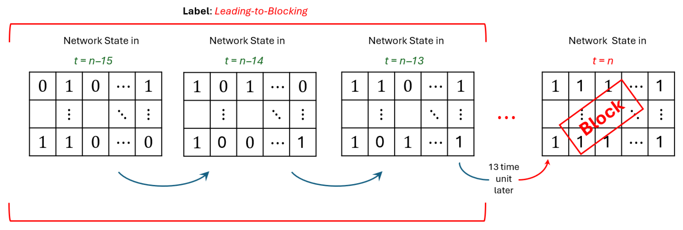
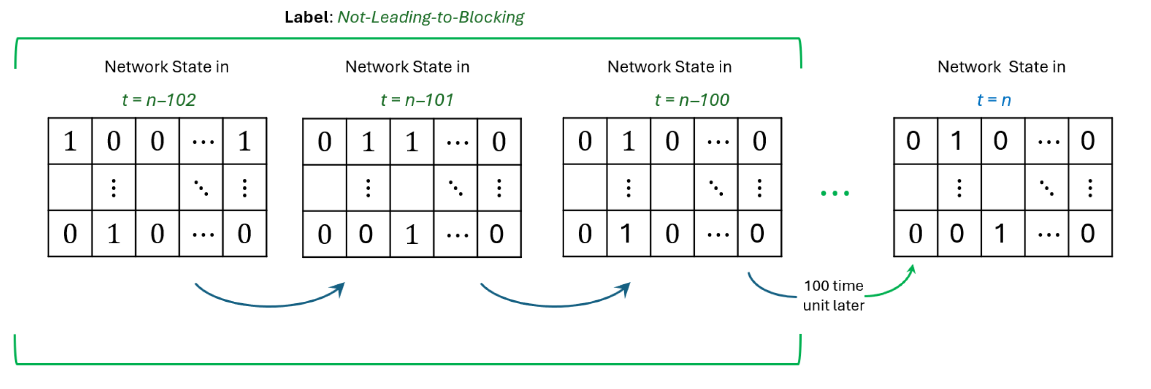
• Data preparation: From all collected snapshots, relevant data is selected: specifically, snapshots just prior to blocking events (13, 14, and 15 time units before) and snapshots not associated with blocking for at least 100 subsequent time units.
• Feature selection and data analysis: Each snapshot is represented as an $l\times s$ matrix (links × frequency slots), which serves as the feature set. Data analysis is performed to identify patterns associated with upcoming blocking events.
• Data preprocessing: Snapshots are reshaped to match the deep learning input requirements and organized into temporal sequences. The dataset is split into training (80%), validation (10%), and testing (10%) sets and labeled as leading-to-blocking or not-leading-to-blocking for 100 time units. This split ratio balances the need for a sufficiently large training set to prevent underfitting while retaining enough validation samples for hyperparameter tuning and early stopping. The traffic samples are generated under homogeneous stochastic processes (Poisson arrivals, exponential holding times), making the 10% validation set representative.
• Model training: Deep learning models are trained on the processed data to learn mappings from network state features to the probability of a future blocking event.
• Model testing: The trained CNN–BiLSTM and CNN–LSTM models are evaluated on unseen data to assess their predictive performance in identifying blocking events at least 13 time units before they occur.

CNN–LSTM and CNN–BiLSTM hybrid models combine spatial pattern detection (CNN) with temporal sequence modeling (LSTM/BiLSTM).

3. Network Simulator and Data Generation

The blocking rate in elastic optical networks depends on both topology (e.g., the number of nodes and links, path lengths, and the number of frequency slots per link) and traffic characteristics (e.g., offered load, connection size distribution, holding times, and inter-arrival processes). These factors jointly determine the level of spectrum fragmentation and the likelihood of rejecting new requests.

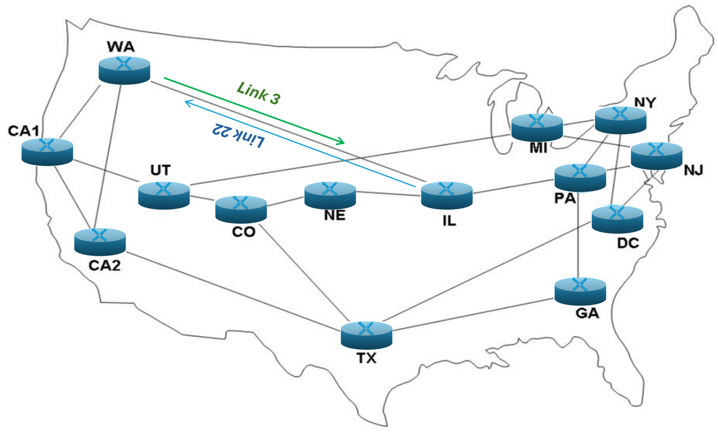
In this study, an EON is simulated using the NSFNET topology (Figure 1) which has been used in the United States and consists of 14 nodes and 21 bidirectional links $(21\times 2=42$ directed links). The 14 nodes in the NSFnet topology represent 14 cities in the USA, and each bidirectional link between cities has independent uplink and downlink channels with their own frequency slots.

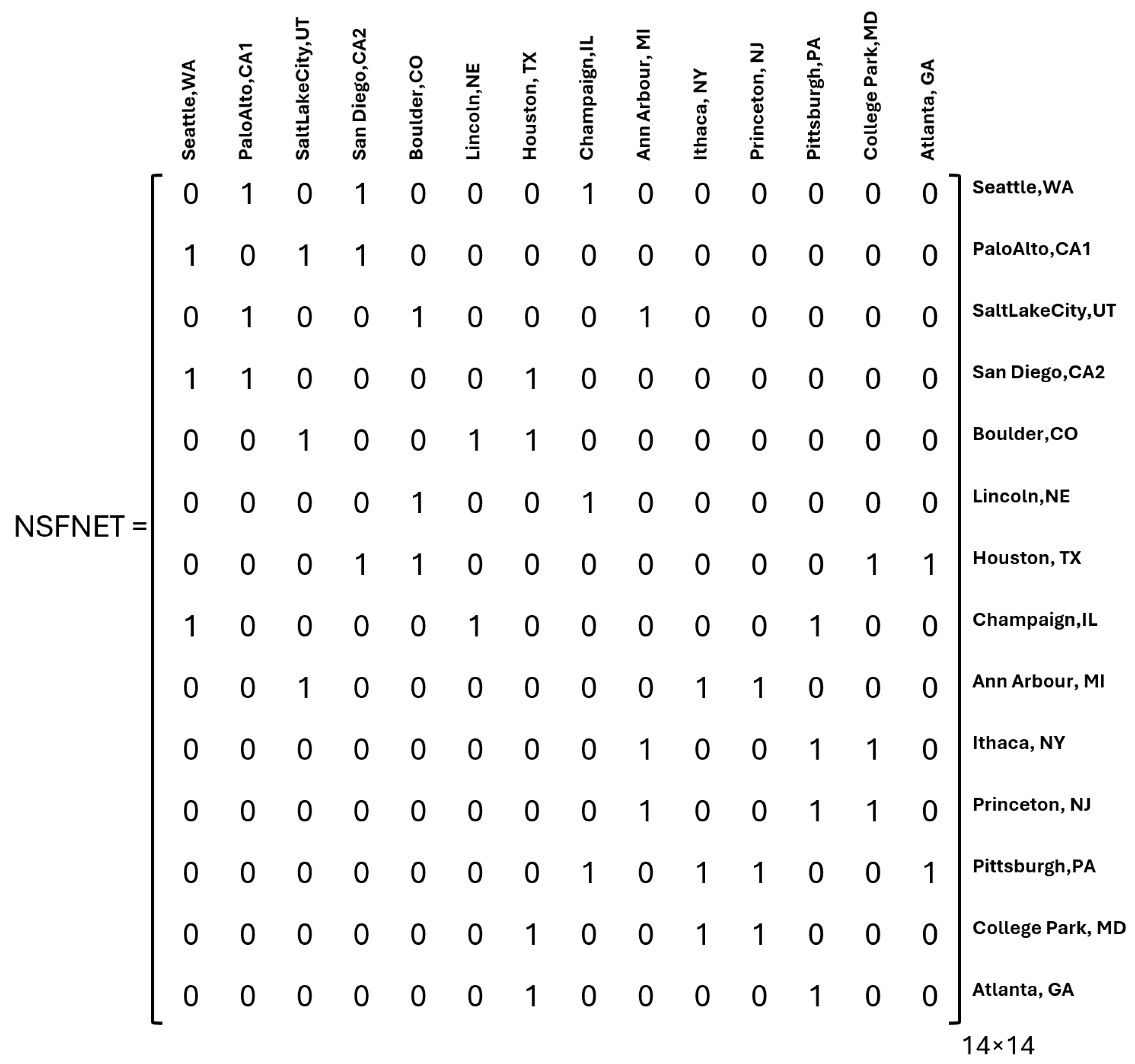
Figure 2 depicts the NSFnet adjacency matrix, which contains 42 ones because, while there are 21 physical links, each link has separate and independent frequency spectra for uplink and downlink directions, resulting in 42 directed links. The NSFnet topology matrix is symmetric due to the bidirectional nature of the links. In the NSFnet topology adjacency matrix, the ones indicate the presence of a direct link between a source node (row) and a destination node (column). For instance, in the first row, the values are $[0,1,0,1,0,0,0,1,0,0,0,0,0,0]$, which indicates that Seattle, WA (node 1) is directly connected to Palo Alto, CA1 (node 2), San Diego, CA2 (node 4), and Champaign, IL (node 8).

For each directed link, a bandwidth of 2 THz is allocated. This bandwidth is divided into equal-sized frequency slots (FS) of 12.5 GHz each. Therefore, each directed link has 160 frequency slots, with each slot providing 12.5 GHz of bandwidth.

The Routing and Spectrum Allocation (RSA) algorithm selects appropriate routes and allocates spectral resources based on network requests [38,39]. The continuity and contiguity of spectrum slots are ensured during spectrum allocation. Traffic simulations were performed using a MATLAB-based simulator (MATLAB R2024a). Statistical characteristics of simulated traffic profiles are as follows:

• Bandwidth: The connection sizes are uniformly distributed between 1FS and 10FS, thereby capturing traffic heterogeneity, which is a typical characteristic of EONs.
• Arrival rate: The connection inter-arrival time (IAT) follows Poisson distribution with average value equal to 1 time unit.
• Holding time: The connection holding times (HTs) follow negative exponential distribution, whose average value is adjusted to reach different network load conditions, which in turn impact blocking probability. The specific HT values used throughout this work are around 250 time units. This leads the network blocking probability to values ranging from 1% to 5%. Changing the connections’ duration parameters would lead the blocking probability to different values, and the prediction time spans explained below should be changed.

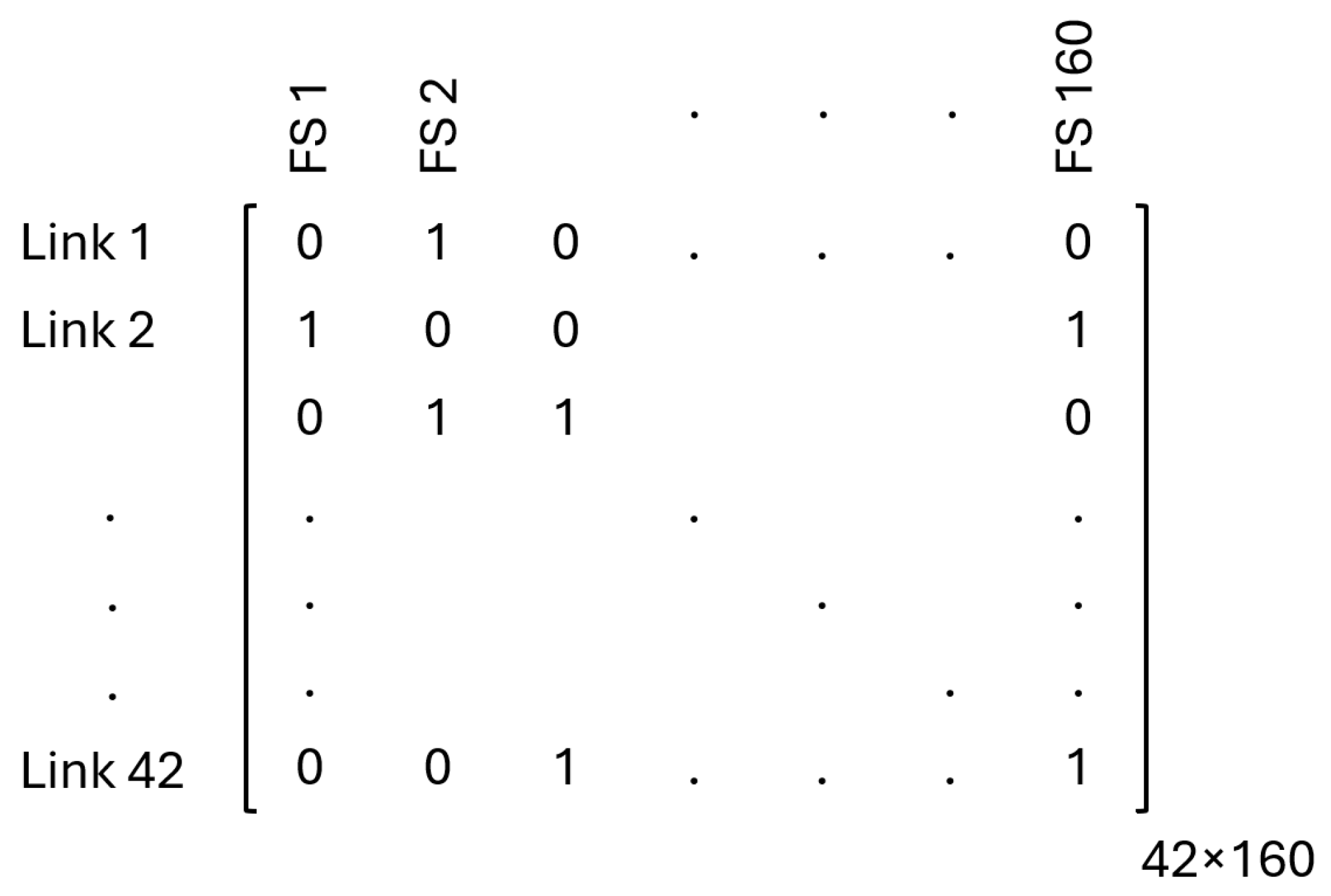
The network state is represented by matrices (42 links × 160 FSs), with snapshots collected continuously, totaling 90,000 samples stored as .csv files.

Data Preparation

The dataset is divided into two classes:

• Leading-to-blocking: snapshots 13 time units before a blocking event.
• Not-leading-to-blocking: snapshots without blocking events within at least 100 subsequent time units.

Three consecutive snapshots taken 15, 14, and 13 time units before a blocking event are labeled as leading-to-blocking (Figure 3). Conversely, three consecutive snapshots for which blocking does not occur within the subsequent 100 time units (taken 102, 101, and 100 time units in the future) are labeled as not-leading-to-blocking (Figure 4). These time parameters could be adjusted accordingly to the network load conditions that impact the blocking.

To allow sufficient time for the network management system to respond and prevent blocking, the blockage should be predicted as early as possible. In this study, for the preliminary analysis, as suggested in [1] we assume that an arbitrary time unit (t.u.) of 13 is sufficient for the network to correct and respond. This value is selected based on the size of the simulated network to illustrate and analyze the concept. In practice, it should be adjusted according to the dynamics of the actual network and the response time of the network administrator. We use the three snapshots taken before the 13 t.u. (i.e., before the blocking) as the training set for blocking prediction. Using three snapshots, rather than a single one, provides the deep learning models with additional information for improved analysis. This number is motivated by a trade-off between predictive accuracy and model complexity [1].

We define not-leading-to-blocking snapshots as those followed by at least 100 t.u. without blocking. This value is arbitrary and serves to illustrate the concept. Assuming a very high number would make the difference between the leading-to-blocking cases overly distinct. The deep learning models are designed to continuously analyze the network and trigger an alarm if a blocking is expected within 13 t.u. However, these values are specific to the IAT and HT used in the simulations of this study and should be adjusted accordingly. To evaluate the model’s performance, we compare its predictions with the actual simulation results.

Data splits include training (80%), validation (10%), and testing (10%). The input data for the models is represented as a numerical matrix of size 42 × 160, capturing a snapshot of the network’s spectral occupancy at a specific time unit (Figure 5). Each element of the matrix indicates the occupancy status of frequency slots across different network links, with occupied frequency slots marked by ones and empty frequency slots represented by by zeros.

4. Proposed Models

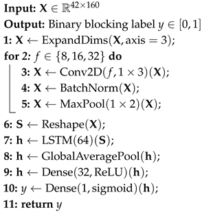
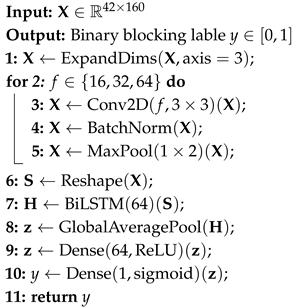
Two deep learning architectures were explored. One model is based on the CNN–LSTM architecture, denoted as Algorithm 1, and the other utilizes the CNN–BiLSTM architecture, referred to as Algorithm 2. Each algorithm possesses different complexity, accuracy, and interpretability. All models process occupancy snapshots $\mathbf{X}\in {\mathbb{R}}^{42\times 160}$, representing the instantaneous optical network state, but differ in their convolutional depth and recurrent capacity.

CNN–LSTM is a family of hybrid deep learning models that combines Convolutional Neural Networks (CNNs) with Long Short-Term Memory (LSTM) networks to analyze data that contains both spatial and temporal patterns. The CNN component extracts spatial features from input data by applying convolution operations, where small filters called kernels move across the input matrix to detect specific patterns. These kernels are trainable parameters that learn to identify important features during the training process.

The Rectified Linear Unit (ReLU) activation function is employed in convolutional layers to introduce nonlinearity into the network, enabling the model to effectively learn complex spatial patterns by activating neurons selectively. Following each convolutional layer, batch normalization is applied to stabilize and accelerate the training process. Batch normalization normalizes the output of each convolutional layer by adjusting and scaling feature distributions, thereby reducing internal covariate shifts, mitigating issues like vanishing gradients, and ultimately leading to improved convergence speed and model stability.

The output of the batch normalization layer is applied to max pooling to simplify and reduce the dimensions of the resulting feature maps. max pooling divides the feature maps into smaller patches and selects the highest value from each patch, effectively preserving the most relevant information. This step reduces the dimensionality of the feature map, lowering computational complexity, decreasing the number of parameters, and improving the model’s robustness by reducing its sensitivity to small variations in the input data.

The extracted spatial features are processed by the LSTM component to capture temporal dependencies. LSTM networks use memory cells and gating mechanisms to remember information across time steps, making them effective for understanding how patterns change over time. Global average pooling is used to convert the variable-length LSTM outputs into fixed-size vectors that can be processed by the final classification layers.

CNN–BiLSTM extends the basic CNN–LSTM architecture by replacing unidirectional LSTM with Bidirectional LSTM (BiLSTM). The BiLSTM processes sequences in both forward and backward directions. This bidirectional processing allows the model to provide a more complete understanding of temporal patterns.

In BiLSTM, one LSTM processes the sequence from start to end, while another processes it from end to start. The outputs from both directions are combined, through concatenating and averaging, to create a comprehensive representation. This approach captures more temporal context compared to unidirectional processing, often leading to better performance in sequence modeling tasks.

After spatial and temporal feature extraction, fully connected layers perform the classification task. These layers consist of neurons that connect to all outputs from the previous layer through learnable weights. To prevent overfitting, a dropout process is employed, which randomly disables a fraction of neurons during training. Activation function ReLU (Rectified Linear Unit) is used to introduce non-linearity, while in the output layer, one neuron and the Sigmoid activation function are used for the classification process.

4.1. Proposed CNN–LSTM (Algorithm 1)

In our proposed CNN–LSTM model, we introduce a reduced-complexity hybrid deep learning algorithm specifically designed for efficient analysis of NSF-NET EON network data containing both spatial and temporal features while significantly reducing computational resources. In a deep learning model, the size of the filters and kernels significantly affects the classification results. Our algorithm is carefully optimized using GridSearchCV to converge better. GridSearchCV is a hyperparameter tuning technique for finding the optimal parameter values for accurate feature extraction and classification.

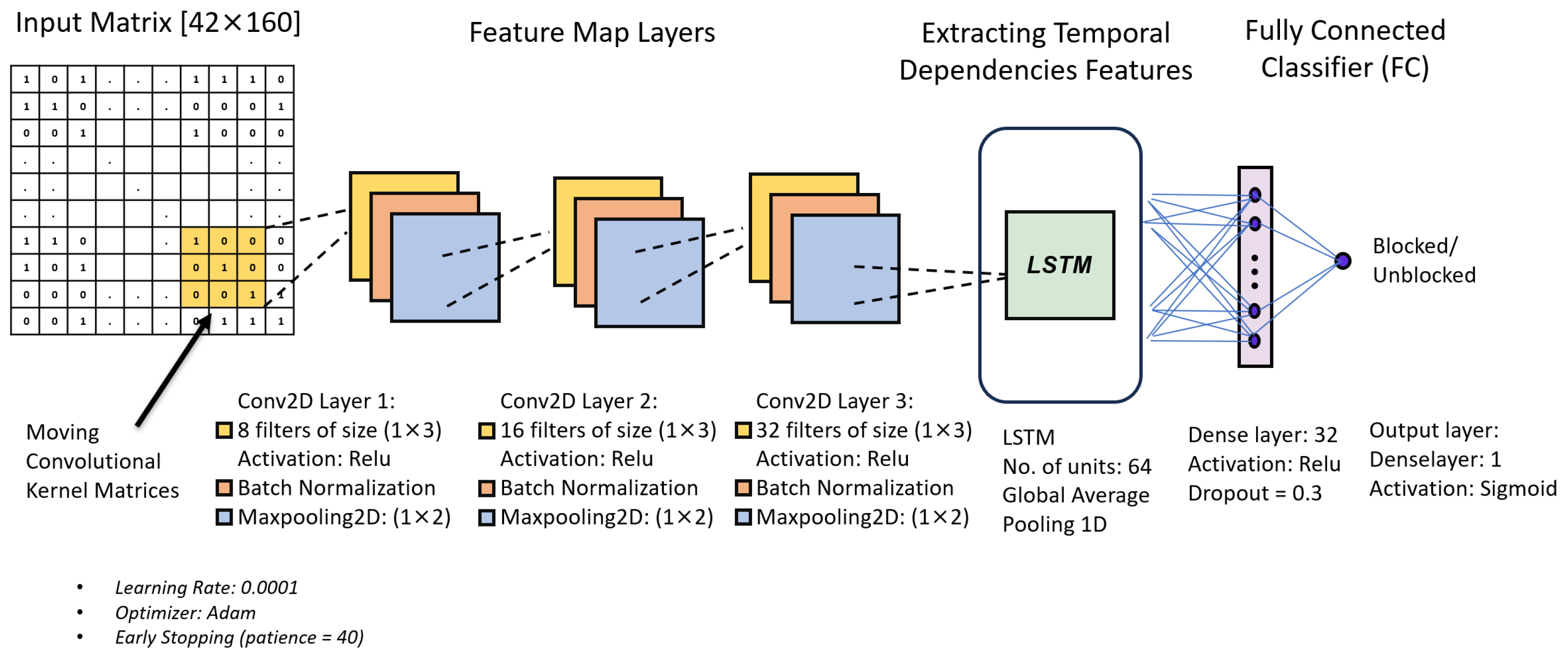
Figure 6 depicts the structure of our proposed CNN–LSTM model. The input to the model is a tensor of shape (42, 160), where 42 represents the number of optical links and 160 denotes the number of frequency slots. This structure allows the model to analyze the spectral usage across multiple links simultaneously. The data is reshaped to ensure compatibility with 2D convolutional operations.

Initially, our method uses a specialized CNN to capture spatial patterns from the input data. The CNN employs three convolutional layers, each using small, row-wise kernels (1 × 3). The first convolutional layer applies eight filters, followed by batch normalization and max pooling (1 × 2), reducing the spectral dimension. Similarly, the second convolutional layer uses 16 filters, and the third uses 32 filters, each followed by batch normalization and max pooling, progressively refining and compressing spectral information.

Subsequently, the extracted features from the CNN layers are reshaped into a sequence format suitable for processing by the LSTM network. The LSTM consists of a single layer with 64 units and is designed to capture dependencies across the set of optical links. A global average pooling operation is applied over the LSTM outputs, reducing the temporal dimension and producing a fixed-size feature vector. This vector is then passed through a dense layer with 32 units and ReLU activation, followed by a dropout (rate = 0.3) to mitigate overfitting. The final dense output layer with sigmoid activation performs binary classification, leading to (blocking vs. unblocking).

The model is trained using the Adam optimizer (learning rate = 0.0001), with early stopping based on validation loss (patience = 40 epochs), and incorporates class weighting based on the frequency of each class in the training set.

The pseudocode of the CNN–LSTM pipeline (Algorithm 1) is as follows:   

Algorithm 1: CNN–LSTM

4.2. Proposed CNN–BiLSTM (Algorithm 2)

To complement the CNN–LSTM model, we introduce a lightweight CNN–BiLSTM architecture. Figure 7 illustrates the architecture of the proposed model. The input is a tensor of shape (42, 160), where 42 denotes the number of optical links and 160 the number of frequency slots. As in the previous model, the data is reshaped to incorporate 2D convolution operations.

After performing hyperparameter tuning as described in Section 5 (within the hyperparameter search space defined in

Table 1. Hyperparameter search space.

Hyperparameter	CNN–LSTM Range	CNN–BiLSTM Range
No. of filters in first convolutional layer	8, 16, 32	16, 32, 64
No. of filters in second convolutional layer	16, 32, 64	32, 64, 128
No. of filters in third convolutional layer	32, 64, 128	64, 128, 256
Size of convolutional kernels	(1,3), (3,3)	(3,3), (5,5)
No. of LSTM/BiLSTM units	32, 64, 128	32, 64, 128
No. of neurons in dense layer units	16, 32, 64	32, 64, 128
Optimizer learning rate	${10}^{-3}$, ${10}^{-4}$, ${10}^{-5}$	${10}^{-3}$, ${10}^{-4}$, ${10}^{-5}$
Training batch size	16, 32, 64	32, 64, 128
Dropout rate	0.2, 0.3, 0.5	0.2, 0.3, 0.5
Max pooling size	(1,2), (2,2)	(1,2), (2,2)

), we obtained the optimal values for the proposed architectures. These optimal hyperparameter values are summarized in

Table 2. Optimal hyperparameter configurations for CNN–LSTM and CNN–BiLSTM models.

Hyperparameter	CNN–LSTM	CNN–BiLSTM
No. of filters in first convolutional layer	8	16
No. of filters in second convolutional layer	16	32
No. of filters in third convolutional layer	32	64
Size of convolutional kernels	(1,3)	(3,3)
No. of LSTM/BiLSTM units	64	64
No. of neurons in dense layer units	32	64
Optimizer learning rate	${10}^{-4}$	${10}^{-4}$
Batch size	32	128
Dropout rate	0.3	0.3
Max pooling size	(1,2)	(1,2)

and illustrated in Figure 7. The model begins with spatial feature extraction layers. This feature extraction module consists of three convolutional layers with progressively increasing filter sizes: 16, 32, and 64. These values are selected based on the hyperparameter tuning analysis, which will be explained in Section 5. Each layer uses 3 × 3 kernels with ReLU activation, followed by batch normalization and max pooling (1 × 2) to reduce dimension, ensuring efficient spectral compression. The output of CNN layers is reshaped to be prepared for the next layer.

A Bidirectional LSTM (BiLSTM) with 64 units is employed to model bidirectional dependencies across optical links. The BiLSTM output is aggregated using global average pooling, followed by a dense layer with 64 units and ReLU activation. A dropout (rate = 0.3) is applied, followed by an output neuron with sigmoid activation for binary classification. Both CNN–LSTM and CNN–BiLSTM models use 64 units in the recurrent layer. In the BiLSTM, the 64 units work in both forward and backward directions, which increases the temporal learning capacity while keeping the same number of units for consistency. The model is trained using Adam optimizer (learning rate = 0.0001) and binary cross-entropy loss, incorporating early stopping (patience = 40 epochs).

The BiLSTM is adopted because spectrum fragmentation evolves with both short- and long-range temporal dependencies; by processing sequences in forward and backward directions, the BiLSTM can capture richer temporal context than a unidirectional LSTM (which processes sequences in a forward direction), leading to improved prediction accuracy.

The pseudocode of the CNN–BiLSTM pipeline is shown in Algorithm 2.   

Algorithm 2: CNN–BiLSTM

4.3. Key Differences Between Proposed Algorithms

The two proposed architectures differ primarily in their CNN depth, recurrent structure, and fully connected layers. Algorithm 1 employs a lightweight CNN architecture, whereas Algorithm 2 utilizes a deeper CNN, impacting their spatial feature extraction capabilities. Additionally, Algorithm 1 incorporates a unidirectional LSTM for temporal modeling, while Algorithm 2 enhances temporal modeling by using a bidirectional LSTM (BiLSTM). Finally, Algorithm 1 uses a fully connected dense layer with 32 units for blocking prediction, whereas Algorithm 2 includes a larger dense layer with 64 units.

Together, these two pipelines systematically explore different neural designs, allowing a clear assessment of their impacts on complexity, accuracy, and interpretability.

5. Hyperparameter Tuning

The performance of deep learning models depends significantly on proper hyperparameter selection. To optimize the CNN–LSTM and CNN–BiLSTM architectures for blocking prediction in elastic optical networks (EONs), we conducted systematic hyperparameter tuning using the GridSearchCV method. This approach ensures that our models achieve optimal performance while maintaining computational efficiency.

GridSearchCV is a systematic technique that explores different combinations of hyperparameters by evaluating model performance across a predefined parameter grid. This method provides a comprehensive search strategy that identifies the optimal parameter configuration for our specific blocking prediction task.

The hyperparameter tuning process follows the following structured approach:

• Define the search space for each hyperparameter.
• Create a grid of all possible parameter combinations.
• Train and evaluate models for each combination using cross-validation.
• Select the hyperparameter configuration (including number of filters, kernel size, number of LSTM/BiLSTM units, dense layer size, learning rate, batch size, dropout rate, and pooling size) that yields the best validation performance.

Table 1 presents the hyperparameters investigated for both CNN–LSTM and CNN–BiLSTM models, along with their respective search ranges.

The total hyperparameter tuning process required approximately 72 h of computation time on 16 GB RAM, AMD Ryzen 7 Microsoft Surface^® Edition 2.00 GHz (Microsoft Corporation, Redmond, WA, USA), evaluating over 18,000 different parameter combinations for both model architectures.

Based on the GridSearchCV results, the optimal hyperparameter configurations for both models are presented in Table 2. These selected configurations represent the final tuned hyperparameters for the CNN–LSTM and CNN–BiLSTM models, and they were used in all subsequent training and evaluation experiments.

It should be noted that the hyperparameters tuned in this work are specific to the NSFNET topology. In general, the optimal values are influenced by both network topology and traffic characteristics. Topological factors such as the number of nodes, link density, and number of frequency slots per link and traffic factors affect the input dimensionality and feature extraction depth required. Consequently, for a larger network or a network with a different topology, hyperparameter re-optimization will be necessary to ensure generalization and robust predictive performance.

Hyper-Parameter Correlation Analysis

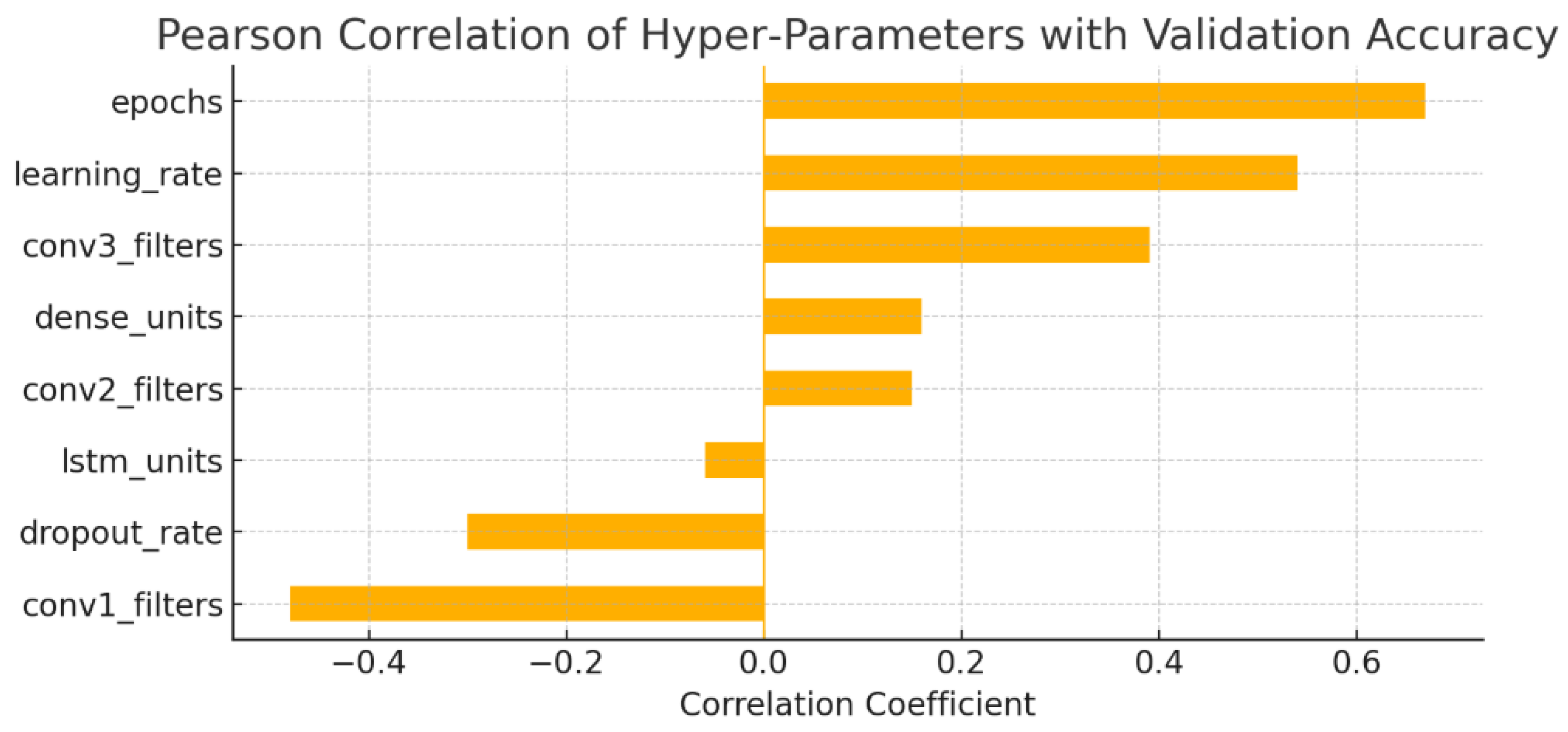
Figure 8 shows the Pearson correlation coefficients between the tuned hyperparameters and the validation accuracy of the CNN–LSTM model. The strongest positive association is observed for the number of training epochs ($\rho \approx 0.67$), suggesting that longer training within the tested range is linked to higher validation accuracy. Learning rate magnitude also shows a positive association ($\rho \approx 0.54$), with step sizes in the moderate ${10}^{-4}-{10}^{-3}$ range tending to achieve better results than smaller values. Increasing the width of the deepest convolutional block (conv3_filters, $\rho \approx 0.39$) was also positively associated with accuracy, while enlarging the first convolutional layer (conv1_filters, $\rho \approx -0.48$) was negatively associated, indicating potential sensitivity to over-parameterization in early layers. Dropout rates above 0.3 showed a negative correlation ($\rho \approx -0.30$), which may reflect the removal of too many informative features. The remaining parameters (dense-layer size, intermediate convolutional width, and LSTM hidden units) show only weak correlations ($\left|\rho \right|<0.20$).

Figure 9 shows the Pearson correlation coefficients between various hyperparameters and validation accuracy for the CNN–BiLSTM model. The number of training epochs has the strongest positive association ($\rho =0.905$), indicating that within the tested range, longer training was linked to higher validation accuracy. Moderate positive associations were also observed for dense layer units ($\rho =0.291$), learning rate ($\rho =0.247$), second convolutional layer filters ($\rho =0.236$), and dropout rate ($\rho =0.226$), suggesting that adjustments to these parameters can influence performance. By contrast, the third convolutional layer filters showed a negative correlation ($\rho =-0.257$), suggesting that excessive depth in convolutional layers may reduce performance in this setting. Hyperparameters, such as LSTM units ($\rho =0.094$) and first convolutional layer filters ($\rho =0.051$), showed only weak associations, implying limited impact on accuracy within the explored ranges. Overall, these results should be interpreted as descriptive trends rather than causal relationships, providing useful guidance on which hyperparameters were most influential during tuning.

6. Validation Criteria

To ensure a comprehensive assessment of the model’s performance in binary classification leading to (blocking vs. unblocking), we utilize the validation metrics explained below.

6.1. Confusion Matrix

The confusion matrix is a table representation that summarizes the model’s classification performance across both classes:

• True Positives (TPs): Correctly predicted “leading-to-blocking” instances;
• True Negatives (TNs): Correctly predicted “Not-leading-to-blocking” instances;
• False Positives (FPs): Incorrectly predicted “leading-to-blocking” when actually “Not-leading-to-blocking”;
• False Negatives (FNs): Incorrectly predicted “Not-leading-to-blocking” when actually “leading-to-blocking”.

It provides deeper insight into the types of classification errors and is especially useful for analyzing class-specific performance.

6.2. Accuracy

Accuracy measures the proportion of correctly classified samples among all samples:

$$\mathrm{Accuracy}={\displaystyle \frac{TP+TN}{TP+FP+FN+TN}}$$

where $TP$, $TN$, $FP$, and $FN$ represent true positives, true negatives, false positives, and false negatives, respectively.

6.3. Loss

The model is trained using binary cross-entropy loss, defined as follows:

$$\mathrm{Loss}={\displaystyle \frac{1}{N}}{\displaystyle \sum _i}\left[-y_{i}log\left({\widehat{y}}_i\right)-(1-y_i)log(1-{\widehat{y}}_i)\right]$$

where $y_i$ is the true label and ${\widehat{y}}_i$ is the predicted probability and N is the number of samples in the batch. Lower loss values indicate better alignment between predictions and ground truth. It is tracked for both training and validation sets to monitor convergence and overfitting.

6.4. Precision

Precision indicates how many of the predicted positive instances are actually positive:

$$\mathrm{Precision}={\displaystyle \frac{TP}{TP+FP}}.$$

High precision means fewer false positives, which is important in scenarios where false alarms must be minimized. Precision indicates how many of the “leading-to-blocking” predictions were actually correct. High precision reduces false alarms.

6.5. Recall (Sensitivity)

Recall measures how many of the actual positive instances were correctly identified:

$$\mathrm{Recall}={\displaystyle \frac{TP}{TP+FN}}.$$

Recall measures the model’s ability to detect all actual positive cases (“leading-to-blocking”). High recall indicates that most “leading-to-blocking” cases are detected, which is critical in ensuring blocked connections are not missed.

6.6. F1-Score

The F1-score is the harmonic mean of precision and recall:

$$F1=2·{\displaystyle \frac{\mathrm{Precision}·\mathrm{Recall}}{\mathrm{Precision}+\mathrm{Recall}}}.$$

It provides a balanced measure when there is a trade-off between precision and recall. It is a single metric that accounts for both false positives and false negatives.

By analyzing all these metrics together, we can be confident that the model works well in terms of accuracy, stability, and error.

7. Training

All models were trained using Adaptive Moment Estimation (Adam), a type of mini-batch stochastic gradient descent algorithm, with a learning rate $\eta ={10}^{-4}$ and mini-batch sizes of 32 and 128 for Algorithm 1 (CNN–LSTM) and Algorithm 2 (CNN–BiLSTM), respectively. To avoid overfitting and enhance training efficiency, early stopping was applied based on validation accuracy with a patience of 40 epochs. The complete Keras models were saved after convergence. CNN–LSTM and CNN–BiLSTM models were trained and validated using the prepared dataset. Predictions were compared with actual simulation outcomes, emphasizing early detection of potential blocking to facilitate proactive network management.

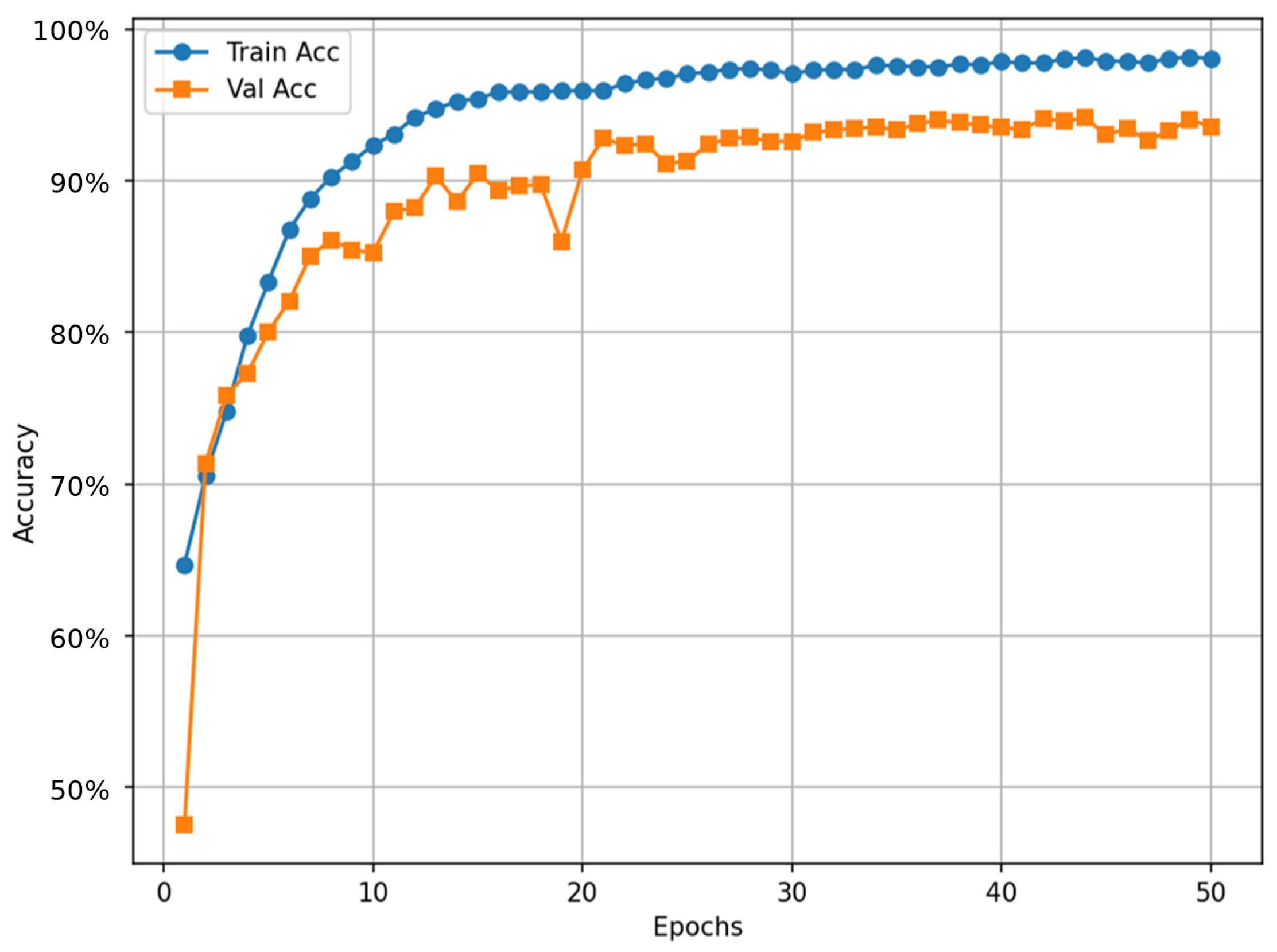
Figure 10 illustrates the training and validation accuracy curves for the CNN–LSTM model over 50 epochs, demonstrating the learning dynamics of the proposed architecture. The training accuracy rises rapidly during the initial epochs, reaching over 90% within the first 10 epochs and gradually converging near 98%. The validation accuracy also exhibits rapid initial improvement, stabilizing around 93%, slightly lower than the training accuracy.

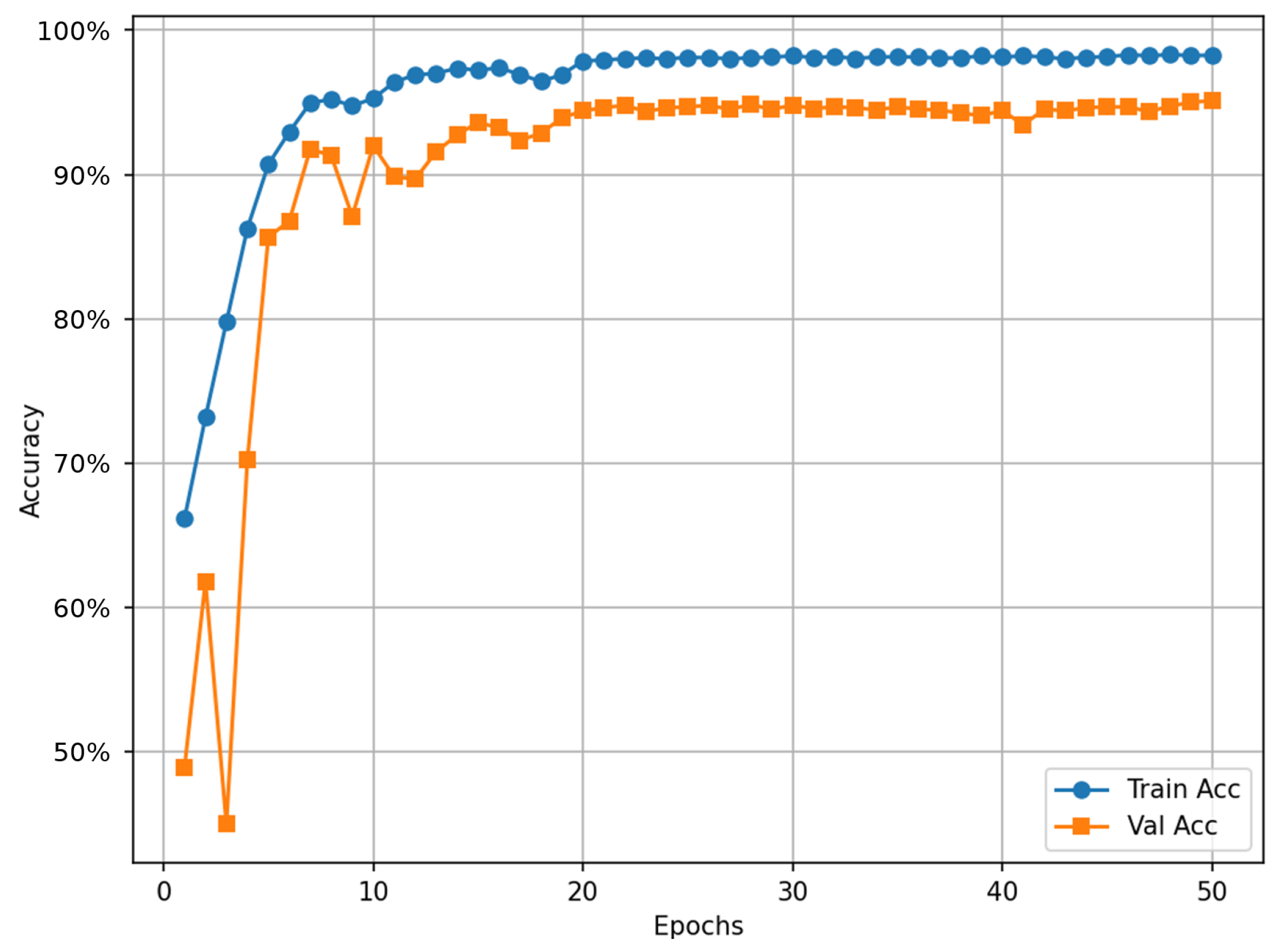
Figure 11 depicts the training and validation accuracy curves of the CNN–BiLSTM model across 50 epochs, highlighting its efficient training dynamics and superior generalization performance. The training accuracy steadily approaches slightly more than 98%, while the validation accuracy experiences initial fluctuations before stabilizing around 95%. The small gap between training and validation curves confirms lower overfitting compared to the CNN–LSTM model.

8. Evaluation and Result

Figure 12 shows the confusion matrix obtained from evaluating the CNN–LSTM model on the test dataset, providing a clear visualization of the model’s predictive performance. The model correctly predicted 839 instances as blocking (True Positives) and accurately classified 1078 instances as non-blocking (True Negatives), demonstrating its robustness. However, it incorrectly classified 77 non-blocking events as blocking (False Positives), and 75 blocking events were misclassified as non-blocking (False Negatives). The overall accuracy reached approximately 92.65%, with precision and recall values of approximately 91.59% and 91.79%, respectively, highlighting the model’s strong capability to accurately detect blocking scenarios while maintaining a balanced error distribution between false alarms and missed detections.

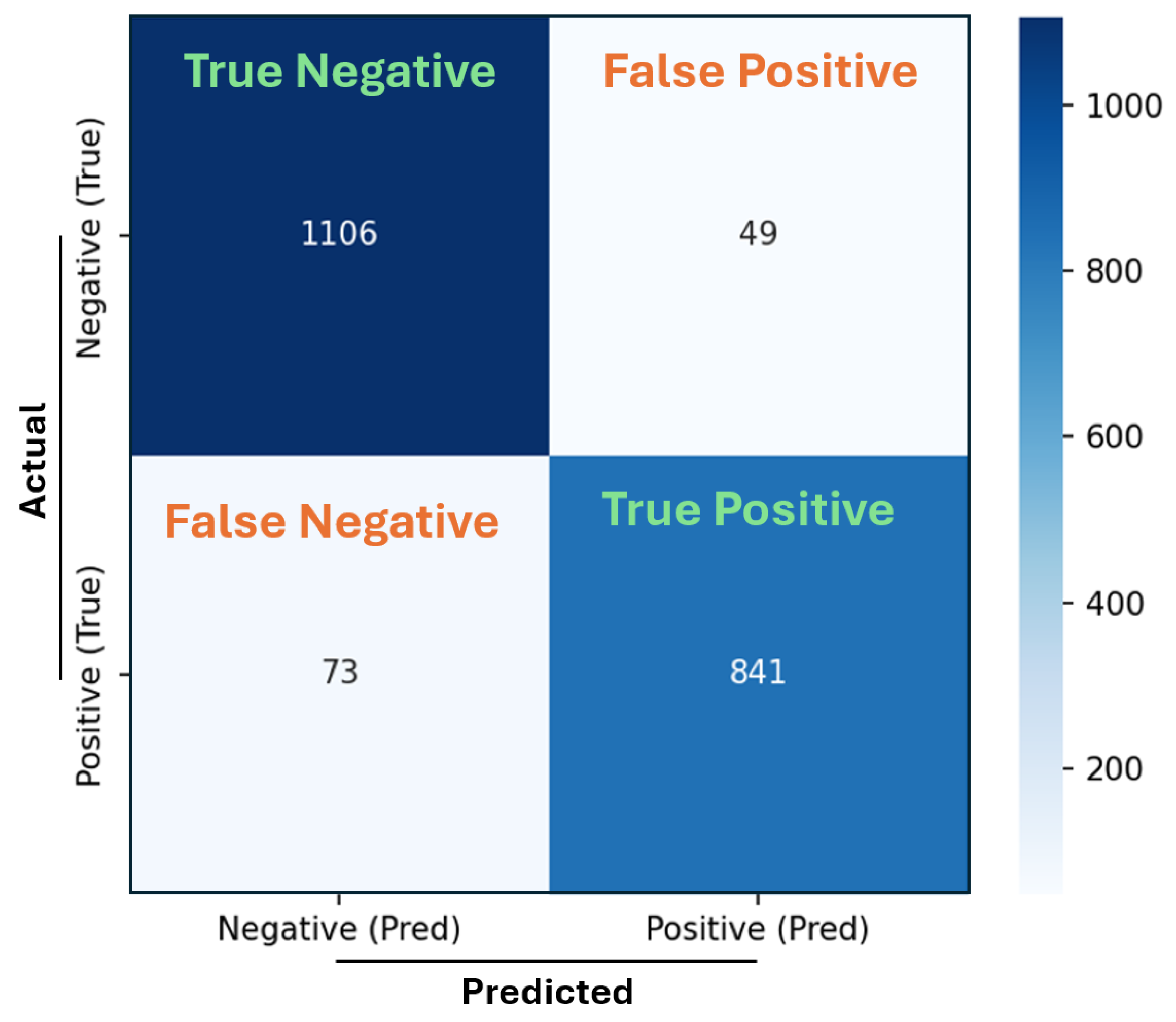
Figure 13 presents the confusion matrix for the CNN–BiLSTM model evaluated on the test dataset, clearly illustrating its superior predictive accuracy. The model correctly identified 841 blocking events as True Positives and 1106 non-blocking events as True Negatives, indicating strong predictive performance with high accuracy, precision, and recall. The model generated fewer incorrect predictions, with only 49 False Positives and 73 False Negatives. Consequently, the CNN–BiLSTM achieved an impressive accuracy of approximately 94.10%, with high precision and recall rates of approximately 94.49% and 92.01%, respectively, underscoring its effectiveness in accurately and consistently predicting blocking scenarios while significantly minimizing false alerts and missed events.

8.1. Complexity, Memory, and Accuracy Comparison

Table 3. Comparison of CNN–LSTM and CNN–BiLSTM models in terms of complexity (number of parameters and memory), validation and test accuracy, and computational cost (FLOPs per request).

Model	#Params	Memory	Validation Acc.	Test Acc.	FLOPs/req
CNN–LSTM (Algorithm 1)	∼0.18 M	∼0.71 MB	$0.9356$	0.9265	∼23 M
CNN–BiLSTM (Algorithm 2)	∼0.72 M	∼2.9 MB	0.9511	0.9410	∼150 M

presents an empirical comparison of the proposed CNN–LSTM and CNN–BiLSTM models in terms of complexity, memory usage, validation accuracy, test accuracy, and computational cost measured by FLOPs (floating-point operations per inference request). The CNN–BiLSTM (Algorithm 2) exhibits better predictive performance, achieving higher validation accuracy (0.9511) and test accuracy (0.9410), compared to the CNN–LSTM (Algorithm 1), which achieves validation and test accuracies of 0.9356 and 0.9265, respectively. However, this improved performance comes at the cost of increased model complexity and computational demands: CNN–BiLSTM consists of approximately 0.72 million parameters, requiring around 2.9 MB of memory and approximately 150 million FLOPs per inference request. In contrast, CNN–LSTM offers a more lightweight alternative with roughly 0.18 million parameters, consuming about 0.71 MB of memory and significantly fewer computational resources (∼23 million FLOPs). Thus, Algorithm 1 significantly reduces complexity to suit resource-constrained environments, compromising some predictive power for faster training. Conversely, Algorithm 2 balances complexity and accuracy by reintroducing bidirectional recurrent layers with moderate convolutional depth.

8.2. Complexity Analysis

Table 4. Complexity calculation for the CNN–LSTM model.

Layer	Complexity	Values	Total
Conv2D (8, $1\times 3$)	$\left(k_h{k}_w{C}_{\mathrm{in}}{C}_{\mathrm{out}}\right)+C_{\mathrm{out}}$	$(1\times 3\times 1\times 8)+8$	32
BatchNorm ($C=8$)	$2C$	$2\times 8$	16
Conv2D (16, $1\times 3$)	$\left(k_h{k}_w{C}_{\mathrm{in}}{C}_{\mathrm{out}}\right)+C_{\mathrm{out}}$	$(1\times 3\times 8\times 16)+16$	400
BatchNorm ($C=16$)	$2C$	$2\times 16$	32
Conv2D (32, $1\times 3$)	$\left(k_h{k}_w{C}_{\mathrm{in}}{C}_{\mathrm{out}}\right)+C_{\mathrm{out}}$	$(1\times 3\times 16\times 32)+32$	1568
BatchNorm ($C=32$)	$2C$	$2\times 32$	64
LSTM (64)	$4\left[(D+H)H+H\right]$	$4\left[(640+64)\times 64+64\right]$	180,480
Dense (32)	$\left(U_{\mathrm{in}}{U}_{\mathrm{out}}\right)+U_{\mathrm{out}}$	$(64\times 32)+32$	2080
Dense (1)	$\left(U_{\mathrm{in}}{U}_{\mathrm{out}}\right)+U_{\mathrm{out}}$	$(32\times 1)+1$	33
Grand total			184,705

and

Table 5. Complexity calculation for the CNN–BiLSTM model.

Layer	Complexity	Values	Total
Conv2D (16, $3\times 3$)	$\left(k_h{k}_w{C}_{\mathrm{in}}{C}_{\mathrm{out}}\right)+C_{\mathrm{out}}$	$(3\times 3\times 1\times 16)+16$	160
BatchNorm ($C=16$)	$2C$	$2\times 16$	32
Conv2D (32, $3\times 3$)	$\left(k_h{k}_w{C}_{\mathrm{in}}{C}_{\mathrm{out}}\right)+C_{\mathrm{out}}$	$(3\times 3\times 16\times 32)+32$	4640
BatchNorm ($C=32$)	$2C$	$2\times 32$	64
Conv2D (64, $3\times 3$)	$\left(k_h{k}_w{C}_{\mathrm{in}}{C}_{\mathrm{out}}\right)+C_{\mathrm{out}}$	$(3\times 3\times 32\times 64)+64$	18,496
BatchNorm ($C=64$)	$2C$	$2\times 64$	128
BiLSTM (64)	$2\times \left(4\left[\right(D+H)H+H]\right)$	$2\left(4\left[\right(1280+64)\times 64+64]\right)$	688,640
Dense (64)	$\left(U_{\mathrm{in}}{U}_{\mathrm{out}}\right)+U_{\mathrm{out}}$	$(128\times 64)+64$	8256
Dense (1)	$\left(U_{\mathrm{in}}{U}_{\mathrm{out}}\right)+U_{\mathrm{out}}$	$(64\times 1)+1$	65
Grand total			720,481

provide the detailed complexity analysis of the CNN–LSTM and CNN–BiLSTM models. In Table 3, the CNN–LSTM model shows a lightweight design with about 185k trainable parameters in total compared to the CNN–BiLSTM model. By contrast, Table 4 shows that the CNN–BiLSTM model contains more than 720k trainable parameters. The deeper convolutional stack and larger dense layer further increase complexity. Although this leads to higher memory requirements and computational cost, the richer temporal modeling capacity improves predictive accuracy, as confirmed in the evaluation results. The tables use the following notations (notations used in Table 4 and Table 5):

• $k_h,k_w$: kernel height and width in convolutional layers.
• $C_{in},C_{out}$: number of input and output channels (filters).
• C: number of channels for batch normalization.
• D: input dimension to the recurrent unit.
• H: number of hidden units in the LSTM/BiLSTM layer.
• $U_{in},U_{out}$: number of input and output neurons in a dense (fully connected) layer.

9. Discussion

To achieve a fair comparison, all baseline methods (e.g., KDD, SVM, 1D CNN, and 2D CNN) were re-implemented following the original papers to ensure methodological consistency. Where source code was available, we used it directly; otherwise, we adhered to the algorithmic descriptions. All methods were trained and tested on the same input format (network state matrices with identical slot granularity) and under identical traffic patterns (Poisson arrivals, uniform bandwidth distribution). Performance metrics (blocking probability, execution time) were measured consistently across methods.

Table 6. Performance comparison of CNN–BiLSTM and CNN–LSTM with baseline methods.

Model	Test Accuracy	Test Loss	Macro F1-Score	Weighted F1-Score	Training Time (s)
CNN–BiLSTM (this work)	0.9410	0.1845	0.9401	0.9409	3771
CNN–LSTM (this work)	0.9265	0.2168	0.9255	0.9265	1966
CNN2D [1]	0.9217	0.2281	0.9208	0.9212	23,561
CNN1D [1]	0.8426	0.4201	0.8425	0.8432	135,960
SVM	0.9091	–	0.9082	0.9093	–
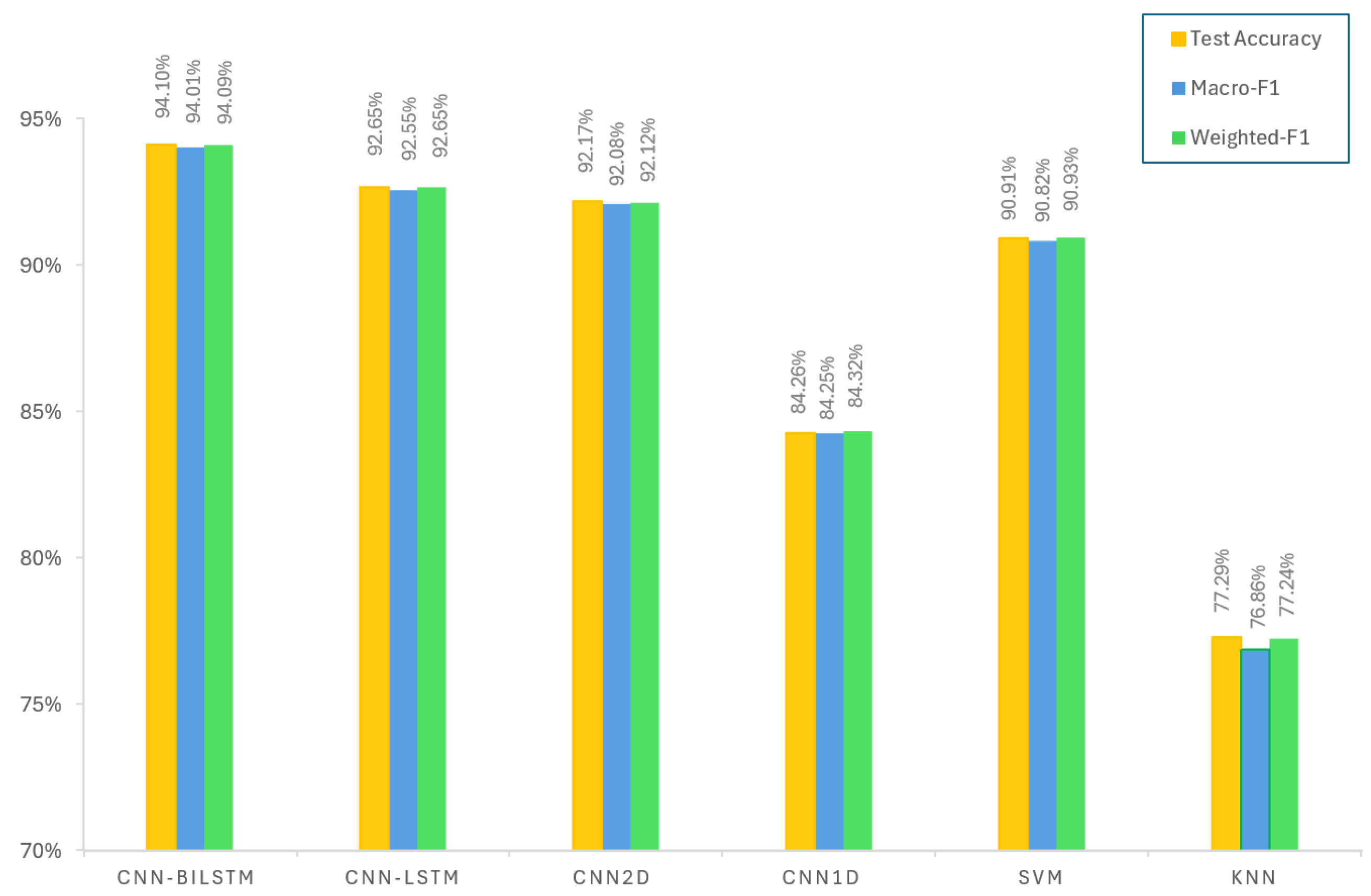
KNN	0.7729	–	0.7686	0.7724	–

and Figure 14 compare the performance of the proposed CNN–BiLSTM and CNN–LSTM models with several baselines, including 2D CNN and 1D CNN from [1], as well as traditional machine learning approaches such as SVM and KNN. The main metrics test accuracy, test loss, macro F1-score, and weighted F1-score show that the CNN–BiLSTM achieves the best results, with a test accuracy of 94.01% and a macro F1-score of 94.01%. This indicates that using 2D CNNs together with a bidirectional LSTM to learn how spectrum fragmentation changes over time provides a clear advantage over unidirectional methods.

CNN–LSTM also performs well, reaching 92.65% test accuracy and weighted F1-scores, but with slightly higher test loss (21.68%) compared to CNN–BiLSTM. The 2D CNN method from [1] shows accuracy (92.17%) but a higher loss (22.81%) compared to our hybrid models, and its training time (23,561 s) is much longer than theirs. The 1D CNN from [1] shows lower performance across all metrics compared to hybrid models and 2D CNNs, and it requires even more training time (135,960 s). The traditional machine learning models SVM and KNN have a lower performance than hybrid deep learning methods. KNN achieves the lowest accuracy (77.29%). These results show that the proposed hybrid CNN–BiLSTM model improves accuracy across different evaluation metrics.

Although the proposed CNN–BiLSTM model needs more training time (3771 s) than the simpler CNN–LSTM (1966 s), its high macro F1-score (94.01%) translates to more accurate alerts for blocking events. These results show that a hybrid approach using both CNNs and recurrent layers can significantly improve blocking predictions while keeping computation manageable. Capturing the local spatial patterns alongside temporal changes in fragmentation is key to achieving a high performance.

10. Conclusions

This paper proposed two models based on CNN–LSTM/BiLSTM. These models are designed to predict spatial fragmentation patterns and their temporal evolution in elastic optical networks. Using a combination of three convolutional layers and a bidirectional LSTM, the proposed method achieved an accuracy of 94.1% and a macro F1-score of 0.94 on the NSFNET dataset. This result outperformed both purely convolutional and standard CNN–LSTM variants.

The model is trained to predict 13 time units ahead of potential blocking events, enabling proactive resource management actions such as spectrum defragmentation or connection rerouting. Additionally, the model is compact, consisting of around 0.72 million parameters, making it suitable for use on standard GPU hardware. The other proposed model, CNN–LSTM, represents a lightweight variant with about 0.18 million parameters and provides reasonable competitive accuracy. However, it has a much shorter training time, suitable for faster and adaptive deployment.

Future work for this research involves expanding the applicability of the proposed model to more complex and larger networks, such as GEANT or other continental-scale mesh topologies, to verify its generalization capability. Applying domain-adaptation methods, such as fine-tuning on selected snapshots, could further enhance the model’s adaptability. Additionally, investigating predictive capabilities over multiple future horizons, such as 5, 10, and 20 steps ahead, would significantly enhance the model’s adaptability and relevance to dynamic, real-world network conditions. Finally, employing graph-aware neural network architectures, such as graph convolutional layers or attention mechanisms on nodes and links, would likely improve the representation of routing constraints that conventional two-dimensional occupancy matrices fail to capture.