On the Capacity of Optical Backbone Networks

Abstract

Optical backbone networks, characterized by using optical fibers as a transmission medium, constitute the fundamental infrastructure employed today by network operators to deliver services to users. As network capacity is one of the key factors influencing optical network performance, it is important to comprehend its limitations and have the capability to estimate its value. In this context, we revisit the concept of capacity from various perspectives, including channel capacity, link capacity, and network capacity, thus providing an integrated view of the problem within the framework of the backbone tier. Hence, we review the fundamental concepts behind optical networks, along with the basic physical phenomena present in optical fiber transmission, and provide methodologies for estimating the different types of capacities, mainly using simple formulations. In particular, we propose a method to evaluate the network capacity that relies on the optical reach to account for physical layer aspects, in conjunction with capacitated routing techniques for traffic routing. We apply this method to three reference networks and obtain capacities ranging from tens to hundreds of terabits/s. Whenever possible, we also compare our results with published experimental data to understand how they relate.

1. Introduction

In recent years, the volume of network traffic has been experiencing almost exponential growth. This phenomenon can be attributed to various factors, such as the widespread adoption of cloud services, the expansion of video distribution platforms and social media, and the emergence of new technologies like 5G and beyond (5G++) [1].

To address this situation, optical networks have emerged as a crucial asset. Optical networks are high-capacity communication infrastructures that utilize light for transmission, processing, and routing of information These networks vary in terms of distance and capacity, falling into several tiers: (1) long-haul networks, such as submarine cables and backbone networks, span extensive geographic distances and offer huge capacities (in the order of dozens of Tbit/s); (2) medium-haul networks, like metro networks, cover cities or metropolitan areas, handling data transmission in the range of hundreds of Gbit/s; (3) short-haul networks, such as access networks, also known as “last-mile networks”, encompass small areas, connecting end-users to the network providers and delivering data rates in the order of a few Gbit/s. In particular, the advent of the fifth-generation fixed network (F5G) allows for supporting access data rates per user larger than 1 Gb/s, with future enhancements promising rates per user up to 10 Gb/s [2].

The most remarkable feature of optical networks is the fact that they use optical fibers as a transmission medium. An optical fiber is a very thin glass filament with a diameter the size of a human hair that has the tremendous advantage of incurring very small losses as the light propagates through it. The first proposal to use optical fibers to carry information was made in 1966 and came from Charles K. Kao [3]. Since that proposal, optical fiber communications have witnessed enormous progress over the last six decades. Several breakthroughs have contributed to that progress; among them, one can refer to the emergence, during the 1990s, of erbium-doped fiber amplifiers (EDFA) and wavelength division multiplexing (WDM), as well as optical coherent detection in the early 20th century [4,5].

Optical amplifiers like EDFAs make it possible to compensate for the fiber losses in the optical domain, avoiding the use of expensive repeaters. Optical coherent detection allows us to increase the number of degrees of freedom to carry information in comparison with traditional direct detection, since it makes use of both the amplitude and phase of the optical signals, while direction detection relies only on intensity. WDM is a fundamental technology in the optical networking field as it enables the transmission of large amounts of data across long distances. It works by simultaneously transmitting multiple optical signals, often referred to as optical channels, through a single optical fiber, with each channel utilizing its own wavelength.

An optical backbone network is structured using interconnected nodes and WDM links in a suitable configuration. Typically, the nodes are based on reconfigurable optical add-drop multiplexers (ROADMs) (for their functionality, see Section 2.2). These ROADMs enable the establishment of paths that traverse the network in optical form, known as lightpaths, which, in turn, correspond to optical channels.

The channel capacity is an important parameter of optical channels. The concept of channel capacity was introduced by Claude Shannon in 1948 [6]. It was defined as the maximum data rate at which information can be reliably transmitted through a noisy channel without errors. The fundamental assumptions behind this definition are that the noise is additive, white, and Gaussian (AWGN), and that the channel is linear, i.e., the capacity always increases with increasing signal power. However, this last assumption does not hold for optical fiber channels, which are non-linear by nature. This behavior implies that the fiber channel capacity does not grow indefinitely; instead, it is limited and reaches a maximum value as the transmitted signal power increases [4,7,8,9].

The problem of estimating the optical channel capacity has been the focus of many studies. Some rely on accurate numerical simulations [9], while others offer detailed analytical models based on either the Gaussian noise (GN) model [10,11,12] or a regular perturbation model [13]. On the contrary, the topic of network capacity has received considerably less attention in the literature, and only recently have some papers been published in this area [14,15,16,17,18]. All these works involved computing the signal-to-noise ratio (SNR) for each optical channel routed in the network, with the capacity of each channel being determined by selecting the modulation format that best suited the SNR and evaluating the corresponding bit rate, with the exception of [17], which though also requiring SNR computations, evaluated the channel capacity using Shannon’s theory instead.

In this paper, we revisit the concept of capacity in optical backbone networks and examine the fundamental principles underlying their operation. We present an alternative approach to evaluate the capacity of optical networks. Rather than using the metric SNR as employed by the other authors, we propose to utilize the metric optical reach, which measures the maximum distance at which an optical channel can propagate effectively, to simplify the computational process. This approach avoids the need to calculate SNRs for all optical channels, which can be cumbersome, especially for large optical networks. Furthermore, we use the network-wide average channel capacity [14] as an intermediate step to assess the network capacity, whereas refs. [15,16,17,18] employ more complex procedures. The paper also relies on an integrated treatment in the sense that it considers various interrelated aspects such as channel capacity, link capacity, and network capacity. A key goal of this work is to understand the trends in capacity evaluation, keeping the analysis as simple as possible, while also investigating how close our results are to the experimental ones reported in the literature.

The rest of the paper is organized as follows: Section 2 provides an overview of the basic principles underlying optical backbone networks and their major physical limitations. Section 3 reviews the concept of channel capacity and introduces the necessary background for determining the spectral efficiency, capacity, and optical reach of an optical channel. In addition, it presents numerical results related to these topics. Section 4 evaluates the link capacity and presents a suitable methodology for computing the network capacity based on the capacitated routing, which is applied afterwards in three reference networks. Finally, Section 5 summarizes and concludes the paper.

2. Basics on Optical Networks and Physical Impairments

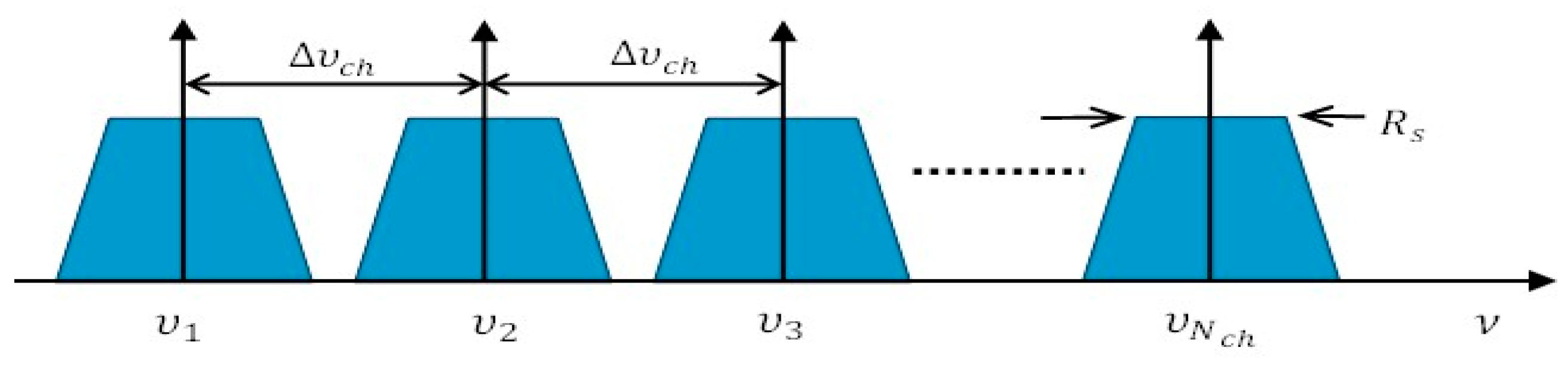
2.1. The Concept of WDM

Figure 1 helps us to understand the concept of WDM. This figure shows $N_{ch}$ optical channels, each characterized by its carrier frequency ${\nu }_k$ (where$k\in \left\{1,\dots ,N_{ch}\right\}$) and symbol rate $R_s$ (in symbols/s or baud), which is related the channel bandwidth through

$$B_{ch}=\left(1+\beta \right)R_s,$$

(1)

with $\beta$ ($0\le \beta \le 1)$ being the roll-off parameter. It is important to note that the frequency $\nu$ in Hz is related to the wavelength$\lambda$ in meters via $\lambda \nu =c$, where $c$ is the speed of the light in the vacuum (approximately $3\times {10}^8\mathrm{m}/\mathrm{s}$). The signal transmitted through the optical channel is assumed to be based on a sequence of symbols at the rate of $R_s$. Each symbol encodes multiple bits of information using the amplitude and the phase of the signal. This process is known as modulation. In a modulation scheme with a symbol constellation of size $M$, each symbol corresponds to ${\log }_{2}M$ bits of information. Examples of modulation schemes used in digital communications include M-ary phase-shift keying (MPSK), which utilizes the phase of the optical signals, and M-ary quadrature amplitude modulation (MQAM), which utilizes both the phase and amplitude.

Figure 1. Spectrum of a WDM signal.

Furthermore, the spacing between the different channels is denoted as $\mathsf{\Delta }{\nu }_{ch}$, subject to the condition $\mathsf{\Delta }{\nu }_{ch}\ge B_{ch}.$ As a consequence, the bandwidth occupied by the WDM signal is equal to $B_{WDM}=N_{ch}\mathsf{\Delta }{\nu }_{ch}$.

When the spacing $\mathsf{\Delta }{\nu }_{ch}$ is very narrow (on the order or tens of GHz) this technique is designated as dense WDM (DWDM). DWDM can be implemented using two approaches: fixed-grid and flexible-grid. In the fixed-grid approach, the channel spacing $\mathsf{\Delta }{\nu }_{ch}$ is kept constant typically at 50 GHz. In contrast, the flexible-grid approach sets $\mathsf{\Delta }{\nu }_{ch}$ as a multiple of an elementary spectral slot of 12.5 GHz and is adjustable according to the requirements of the optical signals being transmitted. DWDM is typically employed in long-haul and high-capacity applications, where it can support over 100 optical channels per fiber. As seen, the number of channels provided depends on $\mathsf{\Delta }{\nu }_{ch}$ and $B_{WDM}$, with the latter parameter being limited by the bandwidth of the EDFAs. Most of the currently deployed DWDM networks operate in the C-band, which is a wavelength range centered around the wavelength of 1548 nm (193.7 THz). Nowadays, standard EDFA technology offers a bandwidth of approximately 4800 GHz (Extended C-band), although more advanced solutions can achieve values up to 6000 GHz (Super C-band). It is worth mentioning that for a channel spacing of 50 GHz, the first solution can support up to 96 channels, while the second one can accommodate up to 120 channels [19].

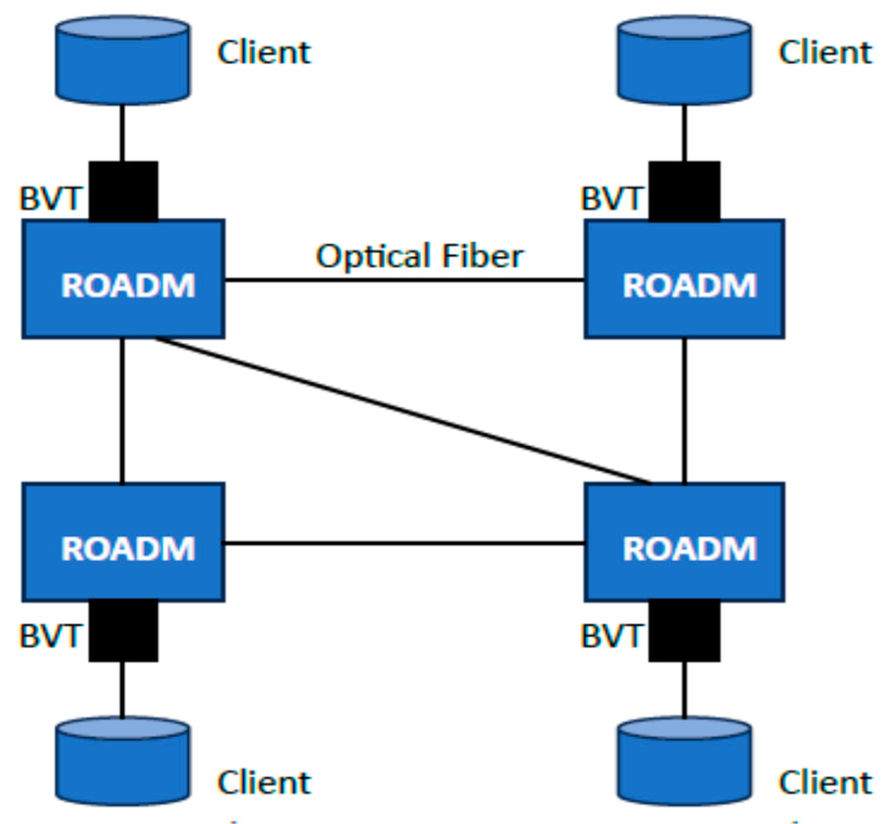
2.2. Optical Network Architecture

This section briefly discusses the architecture of a transparent optical network, with a focus on the backbone tier. Transparent optical networks refer to networks where optical signals are transmitted from the source to the destination without conversion to electrical signals, maintaining their optical nature throughout the network. Therefore, in these networks, all node functionalities (such as multiplexing, switching, routing, etc.) take place in the optical domain, and the node structure is based on ROADMs. The ROADM is responsible not only for locally adding and dropping optical channels, but also for performing optical bypassing through the switching of optical channels from the incoming to the outgoing optical fibers [20]. In addition, they can be remotely configured to establish optical channels and to change their paths and wavelengths, making it a premium function in networks automation. Typically, ROADMs perform demultiplexing and multiplexing of the DWDM signals transmitted in optical fibers and wavelength switching using wavelength selective switches (WSSs). In practice, WSSs are responsible for the dynamism of the ROADM, since they can switch optical channels through the action of the control/management plane.

Figure 2 depicts a simplified architecture of a simple transparent optical network, showing four ROADMs interconnected with optical fibers, as well as bandwidth variable transponders (BVTs) for connecting these network elements to the client equipment. The BVT plays a crucial role in optical networks. First, it is responsible for mapping the signals received on the client side into appropriate containers and adding forward error correction (FEC) codes for error correction purposes. Second, it is responsible for generating optical signals by modulating optical carriers with specific wavelengths on the network side. In this context, BVT can be considered as the source (in the transmitter direction) and the termination (in the receiver direction) of optical channels. BVTs can also be configured remotely to adjust the channel capacity by modifying two key parameters: the number of bits transmitted per symbol, (i.e., the modulation format) and the number of symbols transmitted per second (symbol rate).

Figure 2. Example of an optical backbone network architecture.

A wide range of modulation formats are available, allowing for the trading of spectral efficiency against optical reach. For instance, the utilization of more efficient modulation schemes, such as 128QAM or 64QAM, is limited to optical channels that travel over short distances, while longer distances require the use of less efficient modulation formats, such as quadrature phase-shift keying (QPSK), or even binary phase-shift keying (BPSK). On the other hand, the use of higher symbol rates implies using broader bandwidths, reducing the number of optical channels available in the C-band.

2.3. Major Physical Impairments

Optical reach can be defined as the maximum distance over which an optical signal can be transmitted before its quality of service degrades below a certain metric (bit-error rate (BER), SNR, etc.) threshold. The reach in optical networks is limited by various physical phenomena related to both optical fiber transmission and optical nodes operation. For what concerns fiber transmission, the major impairments are attenuation, chromatic dispersion, and nonlinear effects. On the other hand, optical nodes are affected by impairments such as filter narrowing and crosstalk.

Fiber optic attenuation measures the loss of power in an optical signal as it propagates along an optical fiber and is described by the fiber attenuation coefficient α in dB/km. In the C-band, where it reaches its minimum value, α is typically around 0.2 dB/km. Optical amplifiers are used to compensate for the optical fiber losses. To achieve this, optical amplifiers, typically EDFAs, are placed at discrete intervals along an optical link, with each amplifier exactly compensating the loss incurred by each fiber span. For a link with the length $L$, made up of $N_s$ identical spans, the span length is $L_s=L/N_s$ and the span attenuation is $A_s=\alpha L_s$. Optical amplifiers, besides amplifying the signal, also generate noise known as amplified spontaneous emission (ASE) noise. This noise accumulates as the signal propagates along the link and turns out to be one of the major sources of impairment, significantly affecting the optical reach.

Chromatic dispersion is another limitation and is due to the fact that different wavelengths of a signal travel at different velocities, and therefore, they arrive at the end of the fiber at different times, leading to distortion in the original signal waveform. This occurs because the refractive index of the optical fiber, denoted as $n\left(\lambda \right),$ is wavelength-dependent, and the transmission velocity is defined as $c/n\left(\lambda \right)$. Chromatic dispersion can be characterized using the fiber dispersion coefficient ${\beta }_2$, measured in ${\mathrm{p}\mathrm{s}}^2/\mathrm{k}\mathrm{m}.$ Traditional direction-detection systems, which use simple photodetectors to detect optical signals, require the use of dispersion compensation. This operation is generally achieved by adding sections of a specific type of fiber known as dispersion compensating fiber (DCF) into the standard optical fiber spans. DCF is designed to have the opposite dispersion sign to standard fiber. In coherent detection systems, which employ relatively complex receiver structures, chromatic dispersion can be compensated in the electrical domain through digital signal processing. This solution, which is the one considered in this paper, avoids the use of dispersion compensation in optical domain, leading to the concept of dispersion uncompensated transmission [11].

Another significant impairment in optical fibers is nonlinear interference (NLI) resulting from the Kerr effect. The Kerr effect refers to the dependence of the refractive index of the fiber $n\left(\lambda \right)$ on the transmitted signal power and is quantified by the non-linear fiber coefficient $\gamma$ (measured in ${\mathrm{w}\mathrm{a}\mathrm{t}\mathrm{t}}^{-1}{\mathrm{k}\mathrm{m}}^{-1}$). Unlike attenuation and chromatic dispersion, the Kerr effect is a non-linear phenomenon due to its dependence on optical power. This characteristic makes the optical fiber channel intrinsically non-linear and, in this sense, different from other transmission media used for information transmission that have a linear behavior.

The filter-narrowing effect in optical nodes primarily results from the non-ideal filtering characteristics of WSSs within ROADMs. As a consequence, when an optical signal traverses multiple nodes, the resulting channel bandwidth can be significantly reduced, leading to signal distortion and performance degradation. Despite this situation, there are several methods available in the literature that can be used to mitigate the impact of this impairment (the cascading effects of ROADMs) [21]. Crosstalk in optical networks refers to unwanted interferences between different optical channels. This interference occurs due to imperfect isolation of optical devices like WSSs, resulting in signal leakages responsible for the impairment. Furthermore, crosstalk accumulates as the optical channel traverses multiple network nodes, which increases its damaging effect [22]. However, it is possible to reduce crosstalk to a negligible level by properly designing ROADMs and selecting high-quality WSSs.

3. Channel Capacity

3.1. Capacity of a Communication Channel

According with Shannon’s theory [6], the capacity of a band limited communication channel in the presence of AWGN is given by

$$C_{ch}=B{\log }_2\left(1+\frac{P}{N_{0}B}\right),$$

(2)

where $C_{ch}$ is the channel capacity in bits per second (bit/s), $B$ is the channel bandwidth in Hz, $P$ is the average signal power in watt, and $N_0$ is the noise power spectral density (PSD) in watt/Hz. The signal transmitted through the channel is assumed to be based on a sequence of symbols transmitted at the symbol rate of $R_s$. Each symbol encodes multiple bits of information by modulating the amplitude and/or the phase of the signal.

The minimum bandwidth that a modulated signal can have to allow transmission without inter-symbol interference is defined by the Nyquist criterion and is equal to $R_s$[4]. For such minimum bandwidth, the signal-to-noise ratio becomes

$$SNR=\frac{P}{N_0{R}_s},$$

(3)

and the channel capacity can be written as

$$C_{ch}=R_s{\log }_2\left(1+SNR\right).$$

(4)

3.2. Capacity of an Optical Channel

As previously mentioned, an optical channel can be seen as a communication pathway for transmitting information in the optical domain from a sender to a receiver, using an optical fiber as a transmission medium. This channel is characterized by its carrier frequency ${\nu }_c$in Hz and its occupied bandwidth $B_{ch}$ in Hz, whose minimum value is equal to $R_s$, as discussed earlier.

The capacity of an optical channel is defined as the maximum data rate at which the information can be effectively transmitted through the channel. This capacity is typically expressed in bit/s. Equation (4) can also be applied to compute the capacity of an optical channel, denoted as $C_{ch}$, under the assumption that the noise sources present in these channels are modelled as AWGN sources.

One important noise source in optical systems is ASE noise. This noise is generated inside of optical amplifiers simultaneously with signal amplification and can be effectively described by a random optical field with statistical properties like those of AWGN noise [9]. The PSD of the ASE noise at the end of a chain of $N_s$amplifiers, spaced by fiber spans of length $L_s$, is given by

$$N_{ase}=N_{s}h{\nu }_c{f}_n\left(a_s-1\right),$$

(5)

where $h$ is Planck’s constant (in joule-second), $f_n$ is the noise figure ($f_n={10}^{F_n/10}$, with $F_n$ in dB), and $a_s={10}^{A_s/10}$.

NLI is another significant noise source caused by the Kerr effect in optical fibers, as seen before. Interestingly, it has been demonstrated in [23] through simulations and experiments that the impact of NLI noise on WDM links, supported in dispersion uncompensated fibers, can also be modeled as additive Gaussian noise. Furthermore, it was shown in [11] that under specific conditions, such as the Nyquist limit, the white noise assumption leads to quite accurate results. Note that such a limit is achieved when all the WDM signal channels have a rectangular spectral width and a frequency spacing $\mathsf{\Delta }{\nu }_{ch}$ equal to $R_s$.This permits the characterization of the NLI noise also as an AWGN process with power spectral density of $N_{nli}$. As the ASE and NLI noises are assumed to be uncorrelated, their power spectral densities simply add, resulting in $N_0=N_{ase}+N_{nli}$. In these circumstances, the received signal-to-noise ratio for a given optical channel can be described as

$$SNR=\frac{P_{ch}}{\left(N_{ase}+N_{nli}\right)R_s},$$

(6)

where $P_{ch}$denotes the average output optical power per channel, which is assumed to be equal to the input power, since all losses are compensated for by optical amplifiers.

A rigorous characterization of $N_{nli}$ is not an easy task, and many studies have been published on this topic (see, for example, [11,23]). Fortunately, some closed-form approximations have also been published [10,11,24], which facilitates the evaluation of $N_{nli}.$ One of these approximations, which is based on the white noise assumption, allows us to write the PSD of the NLI at the end of a fiber link with $N_s$ spans in the following way:

$$N_{nli}={\mu }_n{P}_{ch}^3,$$

(7)

where ${\mu }_n$ is the NLI coefficient given by

$${{\mu }_n\approx \left(\frac{2}{3}\right)}^3{N}_s{\gamma }^2{L}_{ef}\frac{\mathrm{l}\mathrm{n}\left({\pi }^2\left|{\beta }_2\right|L_{ef}{B}_{WDM}^2\right)}{\pi {R_s}^3\left|{\beta }_2\right|},$$

(8)

with the $L_{ef}$ being the span effective length given as

$$L_{ef}=\left(1-\exp \left(-2a_N{L}_s\right)\right)/(2{\alpha }_N),$$

(9)

where $L_s$ is the span length and $a_N$ is the fiber attenuation coefficient in Np/km, i.e., ${\alpha }_N={\alpha }_{\mathrm{d}\mathrm{B}/\mathrm{k}\mathrm{m}}/20{\log }_{10}e$. Another relevant parameter to characterize the optical channel is spectral efficiency, measured in bit/s/Hz, which is defined as [9,10]

$$SE=\frac{C_{ch}}{{\mathsf{\Delta }\nu }_{ch}}=2\frac{R_s}{{\mathsf{\Delta }\nu }_{ch}}{\log }_2\left(1+SNR\right),$$

(10)

where factor 2 stems from the fact that the optical fiber channel supports two optical channels with orthogonal polarizations, commonly referred to as polarization multiplexed (PM) optical channels.

By assuming the Nyquist limit, the spectral efficiency $SE$ can be estimated through closed-form calculations using Equations (5)–(10) by making ${\mathsf{\Delta }\nu }_{ch}=R_s$. Note that this approximation is widely used throughout this paper because, when using ${\mathsf{\Delta }\nu }_{ch}>R_s$, the spectral density term $N_{nli}$ cannot be treated analytically [11], and the closed-form Formula (7) cannot be applied. For this reason, we set${\mathsf{\Delta }\nu }_{ch}$ = 64 GHz in Table 1, instead of a multiple of 12.5 GHz, as it would be in more realistic scenarios.

Table 1. Optical fiber and system parameters.

Parameter	Symbol	Value
Fiber Attenuation Coefficient	$\alpha$	$0.22\mathrm{d}\mathrm{B}/\mathrm{k}\mathrm{m}$
Fiber Dispersion Coefficient	${\beta }_2$	$-21.7{\mathrm{p}\mathrm{s}}^2{\mathrm{k}\mathrm{m}}^{-1}$
Fiber Nonlinear Coefficient	$\gamma$	$1.27{\mathrm{W}}^{-1}{\mathrm{k}\mathrm{m}}^{-1}$
Carrier Frequency	${\nu }_c$	$193.41\mathrm{T}\mathrm{H}\mathrm{z}$
Carrier Wavelength	${\lambda }_c$	$1550 \mathrm{n}\mathrm{m}$
Span length	$L_s$	$80\mathrm{k}\mathrm{m},100\mathrm{k}\mathrm{m}$
EDFA noise figure	$F_n$	$5\mathrm{d}\mathrm{B}$
Symbol rate	$R_s$	$64\mathrm{G}\mathrm{b}\mathrm{a}\mathrm{u}\mathrm{d}$
Channel Spacing	${\mathsf{\Delta }\nu }_{ch}$	$64\mathrm{G}\mathrm{H}\mathrm{z}$
Number of Channels	$N_{ch}$	$75$
WDM bandwidth	$B_{WDM}$	$4800\mathrm{G}\mathrm{H}\mathrm{z}$

The obtained results, considering the parameters given in Table 1, are depicted in Figure 3. This figure plots the spectral efficiency as the function of the channel power $\left(P_{ch}\right)$ for different link lengths, considering $L_s=80\mathrm{k}\mathrm{m}$ (Figure 3a) and $L_s=100\mathrm{k}\mathrm{m}$ (Figure 3b). As can be seen, there is a value of the channel power that maximizes the spectral efficiency (${SE}^{max}$). It can be shown that the value of the optimum launch power per channel is given as [11]:

$$P_{ch}^{opt}=\sqrt[3]{\frac{N_{ase}}{2{\mu }_n}}.$$

(11)

Figure 3. Spectral efficiency versus channel power for various link lengths: (a) span length of 80 km; (b) span length of 100 km.

For $L_s=80\mathrm{k}\mathrm{m}$ we have $P_{ch}^{opt}=0.95\mathrm{d}\mathrm{B}\mathrm{m}$ and ${SE}^{max}=18.3\mathrm{b}\mathrm{i}\mathrm{t}/\mathrm{s}/\mathrm{H}\mathrm{z}$, while for $L_s=100\mathrm{k}\mathrm{m}$ we have $P_{ch}^{opt}=2.4\mathrm{d}\mathrm{B}\mathrm{m}$ and ${SE}^{max}=16.3$ bit/s/Hz. These results show that ${SE}^{max}$ decreases by about 2 bit/s/Hz when the span length increases from 80 km to 100 km because of the increase in the ASE noise power. Another conclusion, we can draw from the figure, is that ${SE}^{max}$ also decreases by about 2 bit/s/Hz for every doubling of the link length, and the value of $P_{ch}^{opt}$ is approximately independent of link lengths. These trends had already been identified in [10].

Figure 4 shows the variation of the maximum values of spectral efficiency (${SE}^{max})$as a function of the total link length. As seen, ${SE}^{max}$ decreases in a linear fashion as a function of the link length, when plotted in a logarithmic scale. The spectral efficiency values were computed using Equation (10), which is derived under the hypothesis that the amplitude and phase of the signal at the channel input follow an ideal Gaussian distribution, meaning it is described by a continuous Gaussian constellation (GC). However, in real systems, the input constellations are based on a set of discrete symbols. For a constellation with $M$ symbols, corresponding, for example, to a modulation format such as PM-MQAM, the ideal spectral efficiency is given by $SE=2{\log }_{2}M$ (in bit/s/Hz), where factor 2 accounts for the presence of two polarizations in the channel, as referred to before. Figure 4 also shows the ideal value of SE for different values of $M$. The crossing points between the modulation’s spectral efficiency and the Gaussian constellation’s spectral efficiency enable the evaluation of an upper bound on the maximum reach achieved for each set of symbols (see Table 2).

Figure 4. Maximum value of the spectral efficient (${SE}^{max})$as a function of the total link length, considering a Gaussian constellation (GC) and other discrete constellations with different numbers of symbols (M): (a) span length of 80 km; (b) span length of 100 km.

Table 2. Values of SE related reach as a function of the number of symbols for a PM-MQAM (@$R_s$ = 64 Gbaud).

Number of Symbols (M)	SE (bit/s/Hz)	${\mathit{C}}_{\mathit{c}\mathit{h}}$ (Gbit/s)	Reach (km) ${\mathit{L}}_{\mathit{s}}$ = 80 km	Reach (km) ${\mathit{L}}_{\mathit{s}}$ = 100 km
4	4	256	15,100	9500
16	8	512	3020	1900
64	12	768	720	450
128	14	896	360	225
256	16	1024	180	--------

The results of Table 2 clearly evidence the trade-off between the cardinality of the constellation (number of symbols) and the maximum reach; as the number of symbols increases, reach decreases significantly. For example, one observes a reach reduction between 75% to 80% when the number of symbols quadruple. This reduction increases further to about 95% when the number of symbols increases 16 times. The values of the maximum reach also decrease when the span length increases. By moving from$L_s$ = 80 km to $L_s$ = 100 km, one observes a reach reduction of about 37%. It is also worth mentioning the fact that the results given in Table 2 are closer to the results of Figure 2 of [25], despite these results having been obtained with a more rigorous approach. The current SE record of 17.3 bit/s/Hz was obtained using a modulation format with 4096 symbols and polarization multiplexing (PM-4096QAM) over 50 km [26], which is quite close to the value of 18 bit/s/Hz shown in Figure 4a) for a length of 80 km. Another remarkable experimental result was the achievement of a SE of 14.1 bit/s/Hz at a reach of 500 km using PM-256-QAM) [27]. These two experimental results confirm the previously mentioned trend: a reduction in the reach by approximately 90% when the number of symbols increases by a factor of 16.

According to Equation (10), the optical channel capacity is related to the channel spacing ${\mathsf{\Delta }\nu }_{ch},$ which permits us to write

$$C_{ch}=SE\times R_s\left(1+\beta \right).$$

(12)

Table 2 also presents values for the channel capacity obtained using this equation, considering the Nyquist limit $\beta =0$.

From Equation (12) it can be concluded that two strategies can be employed to increase $C_{ch}$: (1) increasing the spectral efficiency; (2) increasing the symbol rate. The first strategy suffers from the limitations of spectral efficiency already referred. In this way, it is expected a huge reach reduction for increasing values of the capacity. On the other hand, the second strategy increases the sensitivity to noise and nonlinearities and consequently also reduces the reach. However, this reduction can be compensated for by increasing the channel power so that in the end, we only experience a modest decrease in the reach for higher capacity values. The reason for this behavior is that by increasing the channel power in the same proportion as the symbol rate, the power spectral density ($P_{ch}/R_s$) is kept constant, and in this way, the NLI power does not undergo any change (see Equations (7) and (8)).

To give more insights into the problem, let us analyze what happens if we double the channel capacity, starting, for example, with a capacity of 200 Gbit/s based on a PM-QPSK scheme with a symbol rate of 64 Gbaud. By using the first strategy, it is necessary to double the spectral efficiency by going from PM-QPSK (4 bit/s/Hz) to PM-16QAM (8 bit/s/Hz) in order to achieve 400 Gbit/s. However, the last modulation scheme is more sensitive to both noise and nonlinearities, requiring as a consequence a SNR 6.8 dB higher (see Table 3). Therefore, the number of spans supported by PM-16QAM is approximately 4.8 times smaller than that supported by PM-QPSK, which translates into a reach reduction of about 80%, in line with the results given above. Alternatively, we can go to 400 Gbit/s by doubling the symbol rate to 128 Gbaud and keeping the modulation PM-QPSK. In this case, the 50% reduction in reach due to the increases in the noise power (see Equation (6)) can be compensated for by doubling the channel power, ensuring that the reach remains unchanged. A more rigorous analysis of the impact of NLI noise has shown that achieving total reach compensation is unattainable, and in reality, there is an 8% reduction in reach when duplicating the symbol rate (see Figure 2 in [28]).

Table 3. Values of SNR (@${BER}_{pre-FEC}={10}^{-3}$).

Modulation	SNR (dB)
BPSK	6.77
QPSK	9.78
8QAM	14.38
16QAM	16.54
32QAM	20.56
64QAM	22.55
128QAM	26.44

These trends suggest that the optimal strategy for achieving greater optical channel capacities, especially in long-haul networks, is to prioritize increasing symbol rates rather than focusing primarily on spectral efficiencies. Of course, the increase in the symbol rates comes at the cost of requiring larger channel bandwidths, which, in turn, implies a reduction in the number of channels in DWDM transmission. Furthermore, higher symbol rates come at the cost of higher power dissipation rates in the application-specific integrated circuits (ASIC) used in the BVTs [29].

It is important to note that the increase in symbol rates is a current active area of research, with numerous experimental demonstrations yielding results ranging from 100 to 200 Gbaud [30,31,32].

3.3. Optical Reach Evaluation with the Gaussian Model

In our previous analysis, we determined an upper bound for the optical reach as a function of the number of symbols using the spectral efficiency of a signal with a Gaussian constellation. A more realistic approach for assessing optical reach involves using a metric like BER, specifically the BER evaluated before the FEC operation (pre-FEC BER) that takes place inside the BVTs.

In this study, we assume that the threshold is ${BER}_{pre-FEC}={10}^{-3}$. By using the expressions that relate the BER performance with SNR for QPSK [33] and MQAM [34], we arrive at the values given in Table 3.

It also important to be able to determine the data bit rate associated with each modulation scheme, which is given as [4]

$$R_b=2R_s^{\prime }{\log }_{2}M,$$

(13)

where $R_s^{\prime }$ is the net payload symbol rate, which is defined as $R_s^{\prime }=R_s/(1+OH)$, with $OH$ being the FEC and mapping overhead within BVTs. For the purpose of this analysis, we assume an overhead of 28% and a symbol rate of 64 Gbaud, resulting in $R_s^{\prime }=50\mathrm{G}\mathrm{b}\mathrm{a}\mathrm{u}\mathrm{d}.$By utilizing Equation (6) in conjunction with Equations (5) and (7), along with the parameters given in Table 2 and the optimal channel power values (0.95 dBm for $L_s=80\mathrm{k}\mathrm{m}$ and 2.4 dBm for $L_s=100\mathrm{k}\mathrm{m}$), we are able to determine the maximum number of spans required to meet the specified SNR values given in Table 3. This calculation, in turn, allows us to assess the reach of the corresponding optical channel, with the obtained results presented in Table 4. Note that the results for the reach at $L_s$ = 100 km, as presented in Table 4, are close to those in Table I of [35] for $R_s=64$ Gbaud. Similarly, the results for $L_s$= 80 km match well with the findings illustrated in Figure 8 of [29], once again for $R_s=64$ Gbaud.

Table 4. Optical reach values (@${BER}_{pre-FEC}={10}^{-3}$).

Modulation	Data Bit Rate (Gbit/s)	Reach (km) ${\mathit{L}}_{\mathit{s}}$ = 80 km	Reach (km) ${\mathit{L}}_{\mathit{s}}$ = 100 km
PM-BPSK	100	9500	6000
PM-QPSK	200	4750	3000
PM-8QAM	300	1650	1050
PM-16QAM	400	1000	650
PM-32QAM	500	400	250
PM-64QAM	600	250	150
PM-128 QAM	700	100	-----

4. Link and Network Capacity

4.1. Link Capacity

In an abstract way, an optical network can be described as an undirected graph $G\left(V,E\right),$ with $V=\{v_1,\dots ,v_N$} denoting a set of nodes and $E=\{e_1,\dots ,e_K$} denoting a set of links, where $N=\left|V\right|$ is the number of nodes and $K=\left|E\right|$ is the number of links. As mentioned before, in transparent optical networks, all node functionalities take place in the optical domain, and the nodes are built upon ROADMs. Meanwhile, an optical link represents a physical interconnection between two nodes, implemented using optical fibers and optical amplifiers. In bidirectional links, some fibers are used in one direction and others (typically the same number) in the opposite direction. Each optical fiber supports DWDM signals, meaning it carries a specific number of optical channels. For simplicity purposes, we assume that all channels in the links transmit data at the same bit rate.

The capacity of an optical link is determined by both the capacity of individual optical channels and the count of optical channels $N_{ch}$ that it can accommodate. This count is constrained by either the available bandwidth $B_{WDM}$ or the maximum output power $P_{max}$ of optical amplifiers, with $P_{max}$ being limited by the total power$P_{tot}$ carried by the $N_{ch}$ channels; that is, $P_{tot}={N_{ch}P}_{ch}$. When considering the Nyquist limit (${\mathsf{\Delta }\nu }_{ch}$=$R_s)$, and if all the channels have the same modulation format and symbol rate, one can arrive by applying (10) and (12) to the following expression for the link capacity:

$$C_{link}=2{N_{ch}R}_s{\log }_2\left(1+SNR\right),$$

(14)

where $SNR$ is evaluated through Equations (6)–(8).

Figure 5 plots the link capacity as a function of the channel power for four different symbol rate values. The primary conclusion drawn from this figure is that the maximum link capacity ($C_{link}^{max})$ remains constant regardless of the symbol rate. However, this maximum capacity value shifts to higher power levels with increasing symbol rates. This trend is independent of the link length, although the maximum link capacity decreases when the link length increases. As seen, for $L=400\mathrm{k}\mathrm{m}$, $C_{link}^{max}=65.6\mathrm{T}\mathrm{b}\mathrm{i}\mathrm{t}/\mathrm{s}$, while for $L=800\mathrm{k}\mathrm{m}$, we have $C_{link}^{max}=56.1\mathrm{T}\mathrm{b}\mathrm{i}\mathrm{t}/\mathrm{s}$. Table 5 presents several parameters to provide insight, including the optical channel power value that maximizes the link capacity ($P_{ch}^{opt}$) for each symbol rate. Interestingly, the total optical power value remains the same for all the symbol rates. This value is equal to 19.6 dBm, which is well within the capabilities of commercial EDFAs. Furthermore, Table 6 presents some experimental results, reported in the literature, for both the channel and links capacities at various symbol rates. In particular, the results for a symbol rate of 128 Gbaud are quite impressive, revealing values of 1.49 Tbit/s and 52.1 Tbit/s for the channel and links capacities, respectively. However, a drawback of these results is the achieved distance of only 80 km.

Figure 5. Link capacity versus the optical channel power for various symbol rates: (a) link length of 400 km; (b) link length of 800 km.

Table 5. Channel capacities and optical powers per channel.

Symbol Rate (Gbaud)	${\mathit{N}}_{\mathit{c}\mathit{h}}$	${\mathit{C}}_{\mathit{c}\mathit{h}}$ (Tbit/s) $\mathit{L} = 400\mathbf{k}\mathbf{m}$	${\mathit{C}}_{\mathit{c}\mathit{h}}$ (Tbit/s) $\mathit{L} = 800\mathbf{k}\mathbf{m}$	${\mathit{P}}_{\mathit{c}\mathit{h}}^{\mathit{o}\mathit{p}\mathit{t}}$(dBm)	${\mathit{P}}_{\mathit{t}\mathit{o}\mathit{t}}$ (dBm)
32	150	0.44	0.37	−2.15	19.61
64	75	0.88	0.75	0.89	19.64
96	50	1.31	1.12	2.65	19.64
128	37	1.77	1.52	3.89	19.57

Table 6. Published experimental results for channel and links capacities.

Symbol (Gbaud)	${\mathit{N}}_{\mathit{c}\mathit{h}}$	${\mathit{B}}_{\mathit{W}\mathit{D}\mathit{M}}$	${\mathsf{\Delta }\mathit{\nu }}_{\mathit{c}\mathit{h}}$$\left(\mathbf{G}\mathbf{H}\mathbf{z}\right)$	$\mathit{S}\mathit{E}$ (bit/s/Hz)	${\mathit{C}}_{\mathit{c}\mathit{h}}$ (Tbit/s)	${\mathit{C}}_{\mathit{l}\mathit{i}\mathit{n}\mathit{k}}$ (Tbit/s)	L (km)	Ref.
32	117	4400	37.5	6.7	0.25	29.25	1600	[36]
64	59	4400	75.0	6.7	0.50	29.50	650	[36]
96	41	4100	100.0	10.0	1.00	41.00	100	[37]
128	35	4800	137.5	10.9	1.49	52.15	80	[38]

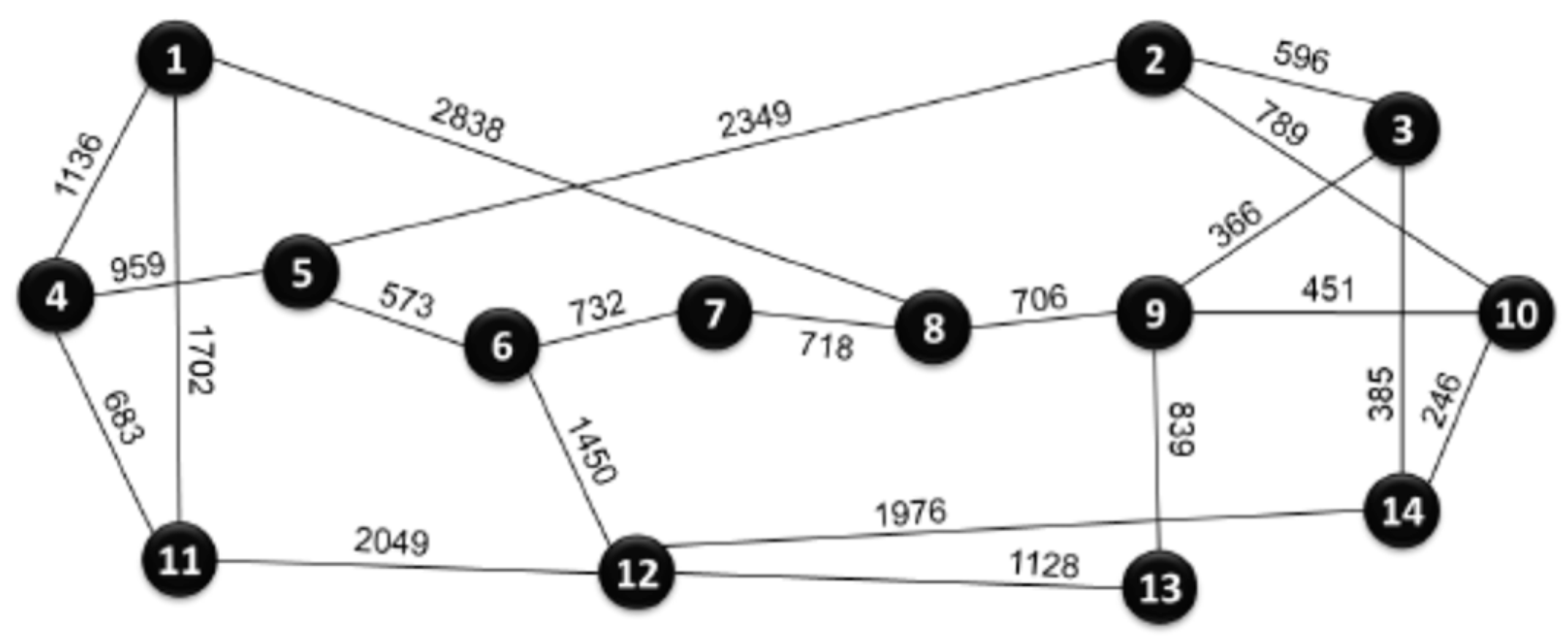
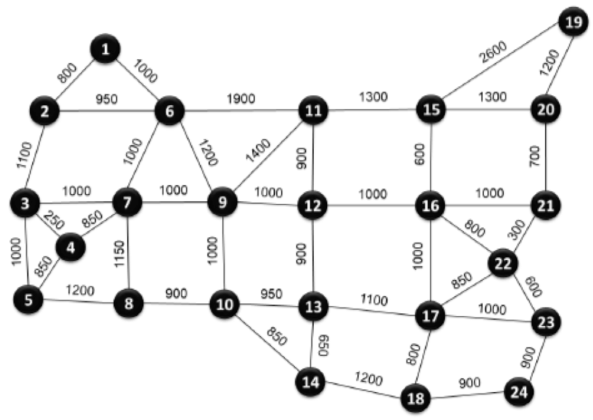
4.2. Network Capacity

Network capacity can be defined as the maximum amount of data that a network can handle per unit of time. This capacity depends on various network properties such as the physical and logical topology (traffic profile), optical reach, link capacity, node structure, etc. Physical topology describes the interconnection pattern of nodes and is typically known in advance. Nodes are considered simultaneously to be the source and destination of traffic. A starting point in the network capacity evaluation is the definition of the traffic demand profile. This profile is defined by the traffic matrix $T=[t_{ij}$], where each entry $t_{ij}$ represents a traffic demand, or in other terms, the volume of traffic flowing from a source node $i$ to a destination node $j$, with $i,j\in V$. In this analysis, it is assumed that the traffic profile is uniform and equal among all node pairs, which corresponds to

$$t_{ij}=\left\{\begin{array}{cc}1& i\ne j\\ 0& i=j\end{array}\right..$$

(15)

Note that this traffic profile describes a full-mesh logical topology in the sense that each node is logically connected to every other node within the network [39]. Another important point in the network capacity evaluation is the link characterization. The link $(i,j)\in E$ can be described by two attributes: (1) length $l(i,j)$, which is a multiple of the span length $L_s$ and equal to $l(i,j)=$ $L_s{N}_s$, as explained above; (2) capacity $c(i,j)$, determined by the number of optical channels $N_{ch}$ available in the links, given by $c\left(i,j\right)=N_{ch}$. As already seen, this number is limited by the bandwidth $B_{WDM}$ and the symbol rate $R_s.$

For each traffic demand, it is necessary to find a path in the physical topology between each pair of nodes. This process is known as routing. Since there are multiple paths between each pair of nodes, the objective is to determine the shortest path using a heuristic like Dijkstra’s algorithm. The shortest path corresponds to the one that minimizes the total path length, defined as the sum of the lengths of all the links traversed by the path. However, in this case, the routing is constrained by the capacity $c\left(i,j\right)$, leading to the concept of the capacitated routing (CR) problem [40]. The objective of this problem is to maximize the number of allocated traffic demands while minimizing the blocking ratio in a network with limited link capacity. In this work, the CR problem is solved through to the following steps:

(1)

Compute the shortest paths:

• Use Dijkstra’s algorithm to find the shortest path for each source–destination pair in the network;
• The total path length is considered as a metric for determining the shortest paths.

(2)

Order the traffic demands:

• Apply a specific sorting strategy (e.g., shortest first, longest first, largest first) to order traffic demands $t_{ij}$.

(3)

Route the demands:

• Route the demands through the precomputed shortest paths obtained in Step 1;
• The routing is conducted according to the orderings considered in Step 2.

(4)

Update residual capacities:

• Whenever a demand is routed, update the residual capacities of all the links traversed by the demand;
• Residual capacity is defined as the difference between the link capacity and its load (number of demands already routed through the link).

(5)

Path selection and blocking:

• First, attempt to use the shortest path obtained in Step 1 for each traffic demand;
• Check the values of residual capacities of all links on the path. If there is enough capacity, use the path;
• If the residual capacities do not allow for using the precomputed path, find an alternative shortest path;

If the computing of an alternative path is not possible because there is not enough capacity, the traffic demand will be blocked.

Furthermore, we assume that each path (also denoted as the lightpath, as referred to before) computed using the CR approach is physically established using an optical channel with a specific wavelength. In other words, a channel $i=\left\{p_i,{\lambda }_i\right\}\in S$ has an associated path$p_i$ and wavelength ${\lambda }_i$ and belongs to the set of optical channels required to implement a logical full-mesh topology $S=\left\{1,2,\dots ,N\left(N-1\right)\right\}$. In this case, one can apply the concepts of channel capacity introduced in Section 3 to compute the total network capacity, which can be written as [17]

$$C_{net}=\sum _{i\in S}{C}_{ch,i},$$

(16)

where $C_{ch,i}$ is the capacity of channel $i$, which, according to (10) and (12), becomes

$$C_{ch,i}=2R_s{\mathrm{l}\mathrm{o}\mathrm{g}}_2(1+SN{R}_i),$$

(17)

with ${SNR}_i$ being the $SNR$ of channel $i$. The ${SNR}_i$ can be readily evaluated using (6), assuming that the optical nodes (ROADMs) are ideal and, as a result, do not affect the calculations. In this context, the number of spans for optical channel $i$ is denoted as $n_{s,i}=L_i/L_s$, with $L_i$ representing the length of path $p_i$. To avoid calculating the ${SNR}_i$ and to reduce computation time, we can take advantage of the analysis undertaken in Section 3 and use the optical reach to obtain the channel’s capacities. For instance, by knowing the lengths of the different paths and utilizing the data from Table 4, we can obtain the capacities of the different channels at two span lengths (80 and 100 km). These capacities are referred to as real capacities, an alternative to ideal or Shannon capacities derived using the spectral efficiencies of the Gaussian constellations shown in Figure 4.

An additional important metric for network analysis is the network-wide average channel capacity, defined as [14]

$${\overline{C}}_{ch}=\sum _{i\in S}{C}_{ch,i}/\sum _{i\in S}{\gamma }_i,$$

(18)

where ${\gamma }_{,i}$ denotes the expected utilization ratio of channel $i$. For the sake of simplicity, it is assumed that ${\gamma }_i=1$ for all $i\in S$. As a result, the sum in the denominator of (18) equals the total number of paths in the network, which, for a full-mesh logical topology, amounts to $N\left(N-1\right).$ With this simplification, the network capacity for a full-mesh logical topology reduces to

$$C_{net}={\overline{C}}_{ch}\times N\left(N-1\right).$$

(19)

For illustrative purposes, we considered the three physical network topologies shown in Appendix A: the COST network ($N=11$, $K=26$, and $\overline{L}=462.6\mathrm{k}\mathrm{m}$), the NSFNET ($N=14$, $K=21,$and $\overline{L}=1211.3\mathrm{k}\mathrm{m}$), and UBN ($N=24$, $K=43$, and $\overline{L}=993.2\mathrm{k}\mathrm{m}$), with $\overline{L}$ being the average link length. The other parameters considered in the analysis are the ones in Table 1. Table 7 and Table 8 give ${\overline{C}}_{ch}$ and $C_{net}$, along with the average path lengths for these networks, considering the real capacities and Shannon capacities, respectively [41]. Note that ${\overline{C}}_{ch}$ was computed using the reach values referred to above, while $C_{net}$ was obtained using Equation (19). As seen, the average channel capacities in the COST239 network are larger than those in the other networks due to the network’s shorter link and path lengths. In fact, the paths in the NSFNET and UBN networks are, on average, 233% and 339% longer than those in the COST239 network, respectively. On the other hand, the UBN network offers a significantly larger capacity compared to the other two networks, despite having the smallest value of ${\overline{C}}_{ch}.$ This is attributed to its capability to support a larger number of optical channels. In practice, the UBN network accommodates 552 optical channels, whereas the NSFNET supports 182 and COST239 only supports 110. Another conclusion we can obtain from these results is that Shannon network capacities outperform the actual network capacities by a factor of about 50%. This is expected, as the Shannon capacity serves as an upper band for the real values. Following the previously mentioned trends, the results show that for a span length of $L_s$ = 80 km, performance is superior compared to $L_s$= 100 km. On average, there is about 13% improvement for real capacities and about 20% improvement for Shannon capacities. On a final note, it can be mentioned that using a more complex methodology [16] reports a capacity of 109.2 Tbit/s for NSFNET, which is quite close to the value of 98.6 Tbit/s given in Table 8.

Table 7. Network-wide average channel and network capacities (real capacities).

Networks	Average Path Length (km)	${\overline{\mathit{C}}}_{\mathit{c}\mathit{h}}$ (80 km) (Gbit/s)	${\overline{\mathit{C}}}_{\mathit{c}\mathit{h}}$ (100 km) (Gbit/s)	${\mathit{C}}_{\mathit{n}\mathit{e}\mathit{t}}$ (80 km) $(\mathbf{Tbit}/\mathbf{s})$	${\mathit{C}}_{\mathit{n}\mathit{e}\mathit{t}}$ (100 km) (Tbit/s)
COST239	682.2	410.9	340.0	45.2	37.4
NSFNET	2268.3	258.2	200.0	47.0	36.4
UBN	2995.9	216.6	168.1	119.6	92.8

Table 8. Network-wide average channel and network capacities (Shannon capacities).

Networks	Average Path Length (km)	${\overline{\mathit{C}}}_{\mathit{c}\mathit{h}}$ (80 km) (Gbit/s)	${\overline{\mathit{C}}}_{\mathit{c}\mathit{h}}$ (100 km) (Gbit/s)	${\mathit{C}}_{\mathit{n}\mathit{e}\mathit{t}}$ (80 km) (Tbit/s)	${\mathit{C}}_{\mathit{n}\mathit{e}\mathit{t}}$ (100 km) (Tbit/s)
COST239	682.2	752.3	672.7	82.8	74.0
NSFNET	2268.3	541.8	459.3	98.6	83.6
UBN	2995.9	496.4	418.1	274.0	230.8

It is worth noting that in our analysis, we used unidirectional traffic demands, i.e., one-way traffic. In this context, a bidirectional flow of information is described by utilizing two unidirectional demands, one for each direction. Alternatively, if bidirectional traffic demands (two-way) are employed, the bidirectional flow can be described with just one demand. The results given in Table 7 and Table 8 for network capacities are based on unidirectional traffic demands, so we can denote these capacities as unidirectional capacities. On the other hand, bidirectional network capacity corresponds to using bidirectional traffic demands. In this case, the values of $C_{net}$ given Table 7 and Table 8 must be halved.

Although Table 5 gives results for the channel capacities considering a link, Table 8 provides results for the average channel capacity considering a network, and it is noteworthy that for $R_s=64\mathrm{G}\mathrm{b}\mathrm{a}\mathrm{u}\mathrm{d}$ and $L=800\mathrm{k}\mathrm{m}$ in the first table, and for $L_s=80\mathrm{k}\mathrm{m}$ and the COST239 in the second table, the capacities are approximately the same (750 Gbit/s). This result arises because the link length of 800 km is close to the average path length of the COST239 network, which is 682 km. It is important to note that a critical point in this analysis is the definition of the span length, which, in both cases in this comparison, is set equal to 80 km. In this way, for $L=800\mathrm{k}\mathrm{m}$, we have 10 spans, while the number of spans varies with the path length. As for the other networks, where the average path lengths are much longer than the link lengths defined in Table 5, it is not possible to make such a comparison.

5. Conclusions

This paper has revisited the problem of estimating the capacity of optical backbone networks, giving attention not only to the channel capacity but also to link and network capacity.

After reviewing the fundamental principles of optical networks and describing the main physical impairments present in these networks, the calculation of spectral efficiency and optical channel capacity was carried out using Shannon’s theory, together with close-form equations available in the literature. Furthermore, an approach was proposed to compute the optical reach, taking into consideration the performance of different modulation schemes.

It was observed that although the maximum values of the spectral efficiency in real networks fall well short of the ideal values, the recent record result of 17.3 bit/s/Hz achieved with M = 4096 symbols (DM-4096QAM) came closer to the theoretical values. The paper also discussed the relationship between channel capacity and variations in the spectral efficiency and symbol rates. It was shown that doubling the capacity through a two-fold increase in spectral efficiency leads to an 80% reduction in the reach. Conversely, when doubling the capacity by doubling the symbol rate, the reach reductions are comparatively modest, not exceeding 10%.

The link capacity was also a focal point of our investigation. This capacity was determined by multiplying the optical channel capacity by the number of channels present in an optical fiber. While the experimental results were not on par with the theoretical predictions, a remarkable value of 52.1 Tbit/s has recently been reported. Finally, the network capacity of three reference networks was computed using a capacitated routing algorithm. The central point of analysis consists in using optical reach values obtained for two scenarios: real capacities and Shannon capacities. It was found that the values of the achieved capacities ranged from tens to hundreds of terabits/s, and that these values are mainly impacted by the path lengths and the number of optical channels accommodated by the network, as well as by the values of the optical reach.

References

- Winzer, P.J.; Neilson, D.T. From Scaling Disparities to Integrated Parallelism: A Decathlon for a Decade. J. Lightw. Technol. 2017, 35, 1099–1115. [Google Scholar] [CrossRef]
- Liu, X.; Li, J.; Wu, X.; Zhu, J.; Zeng, Y.; Liu, D.; Wang, X.; Zhang, D. Fiber-to-the-Room (FTTR) Technologies for the 5th Generation Fixed Network (F5G) and Beyond. In Proceedings of the 2022 IEEE Future Networks World Forum (FNWF), Montreal, QC, Canada, 12–14 October 2022; pp. 351–359. [Google Scholar]
- Kao, K.C.; Hockham, G.A. Dielectric-fibre surface waveguides for optical frequencies. Proc. IEEE 1966, 113, 1151–1158. [Google Scholar] [CrossRef]
- Essiambre, R.-J.; Tkach, R.W. Capacity Trends and Limits of Optical Communication Networks. Proc. IEEE 2012, 100, 1035–1055. [Google Scholar] [CrossRef]
- Winzer, P.J.; Neilson, D.T.; Chraplyvy, A.R. Fiber-optic transmission and networking: The previous 20 and the next 20 years. Opt. Express 2018, 26, 24190–24239. [Google Scholar] [CrossRef]
- Shannon, C.E. A Mathematical Theory of Communication. Bell Syst. Tech. J. 1948, 27, 349–423. [Google Scholar] [CrossRef]
- Mitra, P.P.; Stark, J.B. Nonlinear limits to the information capacity of optical fiber communications. Nature 2001, 411, 1027–1030. [Google Scholar] [CrossRef]
- Ellis, A.D.; Zhao, J.; Cotter, D. Approaching the Non-Linear Shannon Limit. J. Lightw. Technol. 2010, 28, 423–433. [Google Scholar] [CrossRef]
- Essiambre, R.-J.; Kramer, G.; Winzer, P.J.; Foschini, G.J.; Goebel, B. Capacity limits of optical fiber networks. J. Lightw. Technol. 2010, 28, 662–701. [Google Scholar] [CrossRef]
- Bosco, G.; Poggiolini, P.; Carena, A.; Curri, V.; Forghieri, F. Analytical results on channel capacity in uncompensated optical links with coherent detection. Opt. Express 2011, 19, B438–B449. [Google Scholar] [CrossRef]
- Poggiolini, P.; Bosco, G.; Carena, A.; Curri, V.; Jiang, Y.; Forghieri, F. The GN-Model of Fiber Non-Linear Propagation and its Applications. J. Lightw. Technol. 2014, 32, 694–721. [Google Scholar] [CrossRef]
- Bayvel, P.; Maher, R.; Xu, T.; Liga, G.; Shevchenko, N.A.; Lavery, D.; Alvarado, A.; Killey, R.I. Maximizing the optical network capacity. Philos. Trans. R. Soc. A 2016, 374, 2014044. [Google Scholar] [CrossRef]
- Mocozzi, A.; Essiambre, R.-J. Nonlinear Shannon Limit in Pseudolinear Coherent Systems. J. Lightw. Technol. 2012, 30, 2011–2024. [Google Scholar] [CrossRef]
- Souza, A.; Correia, B.; Costa, N.; Pedro, J.; Pires, J. Accurate and scalable quality of transmission estimation for wideband optical systems. In Proceedings of the IEEE 26th International Workshop on Computer Aided Modeling and Design of Communication Links and Networks (CAMAD), Porto, Portugal, 25–27 October 2021. [Google Scholar]
- Vincent, R.J.; Ives, D.J.; Savory, S.J. Scalable Capacity Estimation for Nonlinear Elastic All-Optical Core Networks. J. Lightw. Technol. 2019, 37, 5380–5391. [Google Scholar] [CrossRef]
- Ives, D.J.; Bayvel, P.; Savory, S.J. Routing, Modulation, Spectrum and Launch Power Assignment to Maximize the Traffic Throughput of a Nonlinear Optical Mesh Network. Photon. Netw. Commun. 2015, 29, 244–256. [Google Scholar] [CrossRef]
- Matzner, R.; Semrau, D.; Luo, R.; Zervas, G.; Bayvel, P. Making intelligent topology design choices: Understanding structural and physical property performance implications in optical networks. J. Opt. Commun. Netw. 2021, 13, D53–D67. [Google Scholar] [CrossRef]
- Chen, C.; Xiao, S.; Zhou, F.; Tornatore, M. Throughput Maximization in Multi-Band Optical Networks with Column Generation. arXiv 2023, arXiv:2311.07335. [Google Scholar]
- Deng, N.; Zong, L.; Jiang, H.; Duan, Y.; Zhang, K. Challenges and Enabling Technologies for Multi-Band WDM Optical Networks. J. Lightw. Technol. 2022, 40, 3385–3394. [Google Scholar] [CrossRef]
- Santos, J.R.; Eira, A.; Pires, J. A Heuristic Algorithm for Designing OTN over Flexible-Grid DWDM Networks. J. Commun. 2017, 12, 500–509. [Google Scholar] [CrossRef]
- Rahman, T.; Napoli, A.; Rafique, D.; Spinnler, B.; Kuschnerov, M.; Lobato, I.; Clouet, B.; Bohn, M.; Okonkwo, C.; de Waardt, H. On the Mitigation of Optical Filtering Penalties Originating from ROADM Cascade. IEEE Photonics Technol. Lett. 2014, 26, 154–157. [Google Scholar] [CrossRef]
- Chentsho, P.; Cancela, L.G.C.; Pires, J.J.O. A framework for analyzing in-band crosstalk accumulation in ROADM-based optical networks. Opt. Fiber Technol. 2020, 57, 102238. [Google Scholar] [CrossRef]
- Carena, A.; Curri, V.; Bosco, G.; Poggiolini, P.; Forghieri, F. Modeling of the Impact of Nonlinear Propagation Effects in Uncompensated Optical Coherent Transmission Links. J. Lightw. Technol. 2012, 30, 1524–1539. [Google Scholar] [CrossRef]
- Poggiolini, P.; Carena, A.; Curri, V.; Bosco, G.; Forghierim, F. Analytical Modeling of Nonlinear Propagation in Uncompensated Optical Transmission Links. IEEE Photonics Technol. Lett. 2011, 23, 742–744. [Google Scholar] [CrossRef]
- Gené, J.M.; Perelló, J.; Cho, J.; Spadaro, S. Practical Spectral Efficiency Estimation for Optical Networking. In Proceedings of the ICTON 2023: 23rd International Conference on Transparent Optical Networks, Bucharest, Romania, 2–6 July 2023. Paper Tu.A3.1. [Google Scholar]
- Olsson, S.L.I.; Cho, J.; Chandrasekhar, S.; Chen, X.; Burrows, E.C.; Winzer, P.J. Record-High 17.3-bit/s/Hz Spectral Efficiency Transmission over 50 km Using Probabilistically Shaped PDM 4096-QAM. In Proceedings of the Optical Fiber Communication Conference, San Diego, CA, USA, 11–15 March 2018. Paper Th4C.5. [Google Scholar]
- Chandrasekhar, S.; Li, B.; Cho, J.; Chen, X.; Burrows, E.C.; Raybon, G.; Winzer, P.J. High-spectral-efficiency transmission of PDM 256-QAM with Parallel Probabilistic Shaping at Record Rate-Reach Trade-offs. ECOC 2016-Post Deadline Paper. In Proceedings of the 42nd European Conference on Optical Communication, Dusseldorf, Germany, 18–22 September 2016. Paper Th.3.C. [Google Scholar]
- Poggiolini, P.; Jiang, Y.; Carena, A.; Bosco, G.; Forghieri, F. Analytical results on system maximum reach increase through symbol rate optimization. In Proceedings of the 2015 Optical Fiber Communications Conference and Exhibition (OFC), Los Angeles, CA, USA, 22–26 March 2015. Paper Th3D. [Google Scholar]
- Frey, F.; Elschner, R.; Fische, J.K. Estimation of Trends for Coherent DSP ASIC Power Dissipation for different bitrates and transmission reaches. In Proceedings of the Photonic Networks; 18. ITG-Symposium, Leipzig, Germany, 11–12 May 2017; pp. 137–144. [Google Scholar]
- Li, S.-A.; Huang, H.; Pan, Z.; Yin, R.; Wang, Y.; Fang, Y.; Zhang, Y.; Bao, C.; Ren, Y.; Li, Z.; et al. Enabling Technology in High-Baud-Rate Coherent Optical Communication Systems. IEEE Access 2020, 8, 2020. [Google Scholar] [CrossRef]
- Chen, X.; Raybon, G.; Che, D.; Cho, J.; Kim, K.W. Transmission of 200-GBaud PDM Probabilistically Shaped 64-QAM Signals Modulated via a 100-GHz Thin-film LiNbO3 I/Q Modulator. In Proceedings of the Optical Fiber Communication Conference, São Francisco, CA, USA, 6–10 June 2021. Paper F3C.5. [Google Scholar]
- Yamazaki, H.; Ogiso, Y.; Nakamura, M.; Jyo, T.; Nagatani, M.; Ozaki, J.; Kobayashi, T.; Hashimoto, T.; Miyamoto, Y. Transmission of 160.7-GBaud 1.64-Tbps Signal Using Phase-Interleaving Optical Modulator and Digital Spectral Weaver. In Proceedings of the 2022 European Conference on Optical Communication (ECOC), Basel, Switzerland, 18–22 September 2022. Paper We3D.2. [Google Scholar]
- Pires, J.J.O.; Cancela, L.G.C. Investigating the Impact of Coherent Multipath Interference on Optical QPSK Systems. In Proceedings of the 2017 IEEE International Conference on Communications, Paris, France, 21–25 May 2017. [Google Scholar]
- Cho, K.; Yon, D. On the General BER Expression of One- and Two-Dimensional Amplitude Modulations. IEEE Trans. Commun. 2002, 50, 1075–1080. [Google Scholar]
- Zami, T.; Lavigne, B.; Bertolini, M. How 64 GBaud Optical Carriers Maximize the Capacity in Core Elastic WDM Networks with Fewer Transponders per Gb/s. J. Opt. Commun. Netw. 2019, 11, A20–A32. [Google Scholar] [CrossRef]
- Idler, A.; Buchali, F.; Schuh, K. Experimental Study of Symbol-Rates and MQAM Formats for Single Carrier 400 Gb/s and Few Carrier 1 Tb/s Options. In Proceedings of the 2016 Optical Fiber Communications Conference and Exhibition (OFC), Anaheim, CA, USA, 20–24 March 2016. Paper Tu3A.7. [Google Scholar]
- Matsushita, A.; Nakamura, M.; Yamamoto, S.; Hamaoka, F.; Kisaka, Y. 41-Tbps C-Band WDM Transmission with 10-bps/Hz Spectral Efficiency Using1-Tbps/λ Signals. J. Lightw. Technol. 2020, 38, 2905–2911. [Google Scholar]
- Buchali, F.; Aref, V.; Chagnon, M.; Dischler, R.; Hettrich, H.; Schmid, R.; Moeller, M. 52.1 Tb/s C-band DCI transmission over DCI distances at 1.49 Tb/s/λ. In Proceedings of the 2020 European Conference on Optical Communications (ECOC), Brussels, Belgium, 6–20 December 2020. Paper Mo1E-4. [Google Scholar]
- Pires, J.J.O.; O’Mahony, M.; Parnis, N.; Jones, E. Scaling limitations in full-mesh WDM ring networks using arrayed-waveguide grating OADMs. Electron. Lett. 1999, 35, 73–75. [Google Scholar] [CrossRef]
- Pióro, M.; Medhi, D. Design Modeling and Methods. In Routing, Flow, and Capacity Design in Communication and Computer Networks; Morgan Kaufman Publishers, Elsevier: San Francisco, CA, USA, 2004; pp. 105–149. [Google Scholar]
- Freitas, A. Channel and Network Capacity. Master’s Thesis, University of Lisboa, Lisboa, Portugal, October 2023. [Google Scholar]
- Ribeiro, J. Machine Learning Techniques for Designing Optical Networks to Face Future Challenges. Master’s Thesis, University of Lisboa, Lisboa, Portugal, June 2023. [Google Scholar]