A Survey on Routing Solutions for Low-Power and Lossy Networks: Toward a Reliable Path-Finding Approach

Abstract

Low-Power and Lossy Networks (LLNs) have grown rapidly in recent years owing to the increased adoption of Internet of Things (IoT) and Machine-to-Machine (M2M) applications across various industries, including smart homes, industrial automation, healthcare, and smart cities. Owing to the characteristics of LLNs, such as Lossy channels and limited power, generic routing solutions designed for non-LLNs may not be adequate in terms of delivery reliability and routing efficiency. Consequently, a routing protocol for LLNs (RPL) was designed. Several RPL objective functions have been proposed to enhance the routing reliability in LLNs. This paper analyses these solutions against performance and security requirements to identify their limitations. Firstly, it discusses the characteristics and security issues of LLN and their impact on packet delivery reliability and routing efficiency. Secondly, it provides a comprehensive analysis of routing solutions and identifies existing limitations. Thirdly, based on these limitations, this paper highlights the need for a reliable and efficient path-finding solution for LLNs.

1. Introduction

A Low-power and Lossy Network (LLN) [1] consists of a large number of nodes, often sensor nodes, connected by Lossy channels. The nodes are typically resource-constrained, with limited battery power, memory, and processing capabilities. The channels are unstable, with relatively high packet loss and low packet delivery. LLNs usually have complex traffic patterns that support point–point, point–multi-point, and multi-point–point communication. This means that each node in the network may receive/send packets from/to single or multiple nodes. The network topology can dynamically change over time owing to power depletion and/or node mobility. A typical LLN is shown in Figure 1.

LLNs have several unique characteristics that differ from other types of networks, such as wired networks and ad hoc wireless networks [2,3,4,5]. The characteristics of Lossy channels and nodes, namely their limited energy, memory, and processing capabilities, indicate that the routing solutions designed for non-LLNs may not be adequate in terms of optimising delivery reliability and routing efficiency. By delivery reliability, we mean the ability to successfully deliver data packets from a source node to a destination node with minimum loss and delay as possible. By routing efficiency, we refer to the ability of a routing protocol to transmit data packets between a source node and a destination node in a timely and resource-efficient manner. In other words, it is a measure of how effectively a routing protocol can find the best path to transmit data packets with minimum costs in terms of energy consumption and control overheads.

Routing in LLNs poses a fundamental challenge: determining the optimal path to reach a destination. Over the years, various solutions have sought to address the intricate routing demands in LLNs. However, many of these endeavours often need to account for the full spectrum of factors that influence routing reliability. A routing protocol designed for LLNs should operate within the constraints of Lossy channels and limited node energy and effectively and efficiently achieve the routing function. In other words, all factors that may impact packet delivery reliability and routing efficiency should be considered when making routing decisions. In addition, the routing protocol should also support dynamic topology and link quality changes as caused by power depletion.

In light of these considerations, this paper presents a comprehensive assessment of current solutions for LLNs against performance and security requirements to identify limitations and emphasise the need for a reliable and efficient path-finding solution within the complex network of LLNs. Our research provides a critical analysis of existing routing solutions for LLNs, particularly focusing on the gaps in RPL solutions. We examine the oversight of neglecting essential reliability-effecting factors such as node energy levels and link quality in the path selection process. We thoroughly examine generic routing protocols and RPL objective functions, covering non-malicious and malicious LLNs, to identify areas of improvement for reliable path-finding. Our paper highlights the importance of maximising PDRs by considering the most reliability-effecting factors, even in the presence of malicious nodes. We underscore the absence of solutions capable of making real-time, global optimum decisions that adapt to dynamic network changes. As part of our contribution, we outline a road map for future work that aims to design and implement a robust path-finding solution for LLNs in the presence of PDAs. This forthcoming research endeavours to elevate delivery reliability and enhance routing efficiency in LLNs, bridging the identified gaps in the current state of the art.

In detail, the remainder of this paper is structured as follows. Section 2 illustrates the characteristics of LLNs. Section 3 surveys the generic routing solutions. Section 4 surveys RPL objective functions for non-malicious LLNs and RPL objective functions for malicious LLNs (MLLNs). Section 5 provides a summary of existing surveys on RPL solutions. Section 6 presents further discussions, and Section 7 concludes the paper.

2. Characteristics of Low-Power and Lossy Networks (LLNs)

The term LLN was first introduced by the Internet Engineering Task Force (IETF) group. LLNs typically consist of many sensor nodes interconnected by low-cost and low-data-rate wireless links designed explicitly for it, such as IEEE 802.15.4 [6] and low-power Wi-Fi [7]. Small sensor nodes often have limited central processing unit (CPU), memory, and power resources. These resource limitations create constraints on the (i) maximum code complexity in read-only memory (ROM) and flash, (ii) size of state and buffers in random access memory (RAM), (iii) amount of computation feasible in a period of time, i.e., processing capabilities, and (iv) available energy [8].

The IETF classifies constrained nodes into three classes based on their capabilities: Class 0 (C0), Class 1 (C1), and Class 2 (C2) [9]. C0 nodes are very constrained in memory and processing capabilities. They generally do not have the resources required to be secured against security attacks or to connect directly to the internet. Therefore, C0 nodes often participate in internet communication through gateways or servers. C1 nodes are constrained in code space and processing capabilities but are less constrained than C0 nodes. They have the resources required to communicate without the help of gateways or servers using a protocol stack specifically designed for constrained nodes, such as the Constrained Application Protocol (CoAP) [10] over the User Datagram Protocol (UDP) [11,12]. C1 nodes can be fully integrated into an Internet Protocol (IP) network and support the security functions required on a network. However, memory, code space, and energy resources must be used wisely and efficiently. C2 nodes are the least constrained in terms of memory and processing capabilities. Unlike other classes, C2 nodes can consume less bandwidth and support lightweight and energy-efficient protocols.

Table 1. Classes of constrained nodes.

Class	RAM (Data Size)	ROM/Flash (Code Size)	Example
C0	≪10 KiB	≪100 KiB	Sky mote
C1	∼10 KiB	∼100 KiB	Z1 mote
C2	∼50 KiB	∼250 KiB	Wistmote

shows the different classes of the constrained nodes, their data and code size capabilities, and some examples.

Using constrained nodes to form a network often leads to constraints on the network itself. These constraints on the network can affect (i) routing reliability and (ii) network security. The reliability of routing is often compromised by constraints resulting in high packet loss and low delivery rates owing to Lossy channels and link fragmentation. It may also cause limitations on reaching some nodes over time owing to a lack of energy and topology fragmentation, as nodes may power off at any time. Therefore, LLNs usually exhibit unreliable and unstable links with high packet loss rates and short network lifetimes.

Moreover, constraints on the nodes usually affect network security, making it challenging to secure LLNs using security measures available for wired and unlimited power networks [13]. This makes the task of protecting LLNs against security attacks very challenging, as nodes often do not possess the resources required to implement complex security techniques such as cryptography. The most relevant constraints that may directly limit the ability to secure LLNs are (i) low memory size, which requires a small code size and low code complexity, (ii) low power operation, (iii) low processing capabilities, and (iv) small bandwidth requirements. Given these constraints, security threats impose huge risks as they not only affect network security but may also drain the node resources that are trying to defend against them. Therefore, a security solution for LLNs should balance the trade-off between security and the available resources for the network to perform efficiently.

One of the most common attacks in LLNs is the Packet Dropping Attack (PDA) [14,15,16,17], in which a malicious node joins a network and intentionally drops packets instead of forwarding them. PDAs can be classified into two categories: (i) black-hole and (ii) grey-hole attacks. In black-hole attacks, a malicious node drops all received packets from neighbouring nodes, i.e., control packets and data packets [18,19,20]; meanwhile, in grey-hole attacks, a malicious node selectively drops certain packets and forwards others [21]. One specific form of a grey-hole attack is the Selective Forwarding Attack (SFA), in which a malicious node selectively chooses which packets to discard and when to do so [22]. For example, the malicious node may choose to forward control packets while dropping received data packets for a given duration, such as thirty minutes. Both types of PDA directly affect the (i) availability of network services by isolating nodes from communicating with each other and (ii) routing reliability by dropping packets and reducing packet delivery [23]. The routing information exchanges, i.e., control packets, and forwarding data packets must be available during the entire runtime for the routing protocol to perform correctly. Figure 2 illustrates the two categories of PDAs.

3. Generic Routing Solutions

Most routing protocols are designed for wired networks [24,25] and Mobile Ad-hoc Networks (MANETs) [26,27] in general. The routing protocols can primarily be classified into two main categories: (i) Link-State Routing Protocols (LSRPs) [28,29] and (ii) Distance Vector Routing Protocols (DVRPs) [30,31]. These two categories are discussed in detail in the following sections. A summary of the main generic routing protocols is shown in Figure 3.

3.1. Link-State Routing Protocols (LSRPs)

The LSRP concept was introduced in 1979 by McQuillan [32] to find the best path between a pair of nodes under network topology changes and create stable routing. In LSRP, nodes create a complete network topology map by collecting information from other nodes in the network. Thus, every node maintains routing information to every other node in the network. The first step for the nodes is to send “Hello” messages, also known as keep-alive messages, for neighbour discovery. Then, each node establishes a relationship with its direct neighbours, the first hop, to exchange routing information. This relationship between neighbour nodes is called adjacency, and it can be formed by periodically sending advertisement packets. Advertisement packets are divided into three different types: (i) Link-State Request (LSR), (ii) Link-State Update (LSU), and (iii) Link-State Acknowledgement (LSAck). These advertisement packets contain local topology information about the node itself, directly connected links and the state of those links [33]. The information is then propagated through the entire network using a flooding technique. The collected information is used to (i) produce a Link-State Database (LSDB) for the network topology and (ii) select the best available path, usually the shortest path, between the source and the destination node.

The collected information about the direct neighbours is stored in a table known as the neighbour table. In contrast, the collected information about the entire network topology is stored in the topology table. A third table, namely the routing table, is then created by each node using its own LSDB. The routing table contains information about the shortest available paths to all the advertised neighbours based on some routing metrics. Each entry in the routing table represents a destination node pointing to the next hop, allowing the LSRP to immediately find alternative paths in the case of link failure. To update these tables, LSRP uses the concept of triggered updates, which means that “Hello” messages and advertisements, i.e., control packets, are only resent when topology changes occur in the network. LSRP typically uses the Dijkstra algorithm, i.e., Shortest Path First (SPF), to find the best path between a pair of nodes. The Dijkstra algorithm was created by E. Dijkstra and was published in 1959 to solve the shortest path problem in a directed graph [34]. The algorithm starts at a start node and then searches through the topology map to find the shortest distance between this particular node, the start node, and its direct neighbours in the network. This search process then continues to find the shortest path for all the nodes in the network [35]. In this way, LSRP has the required information to calculate the best available path connecting the source node to any destination node in the network.

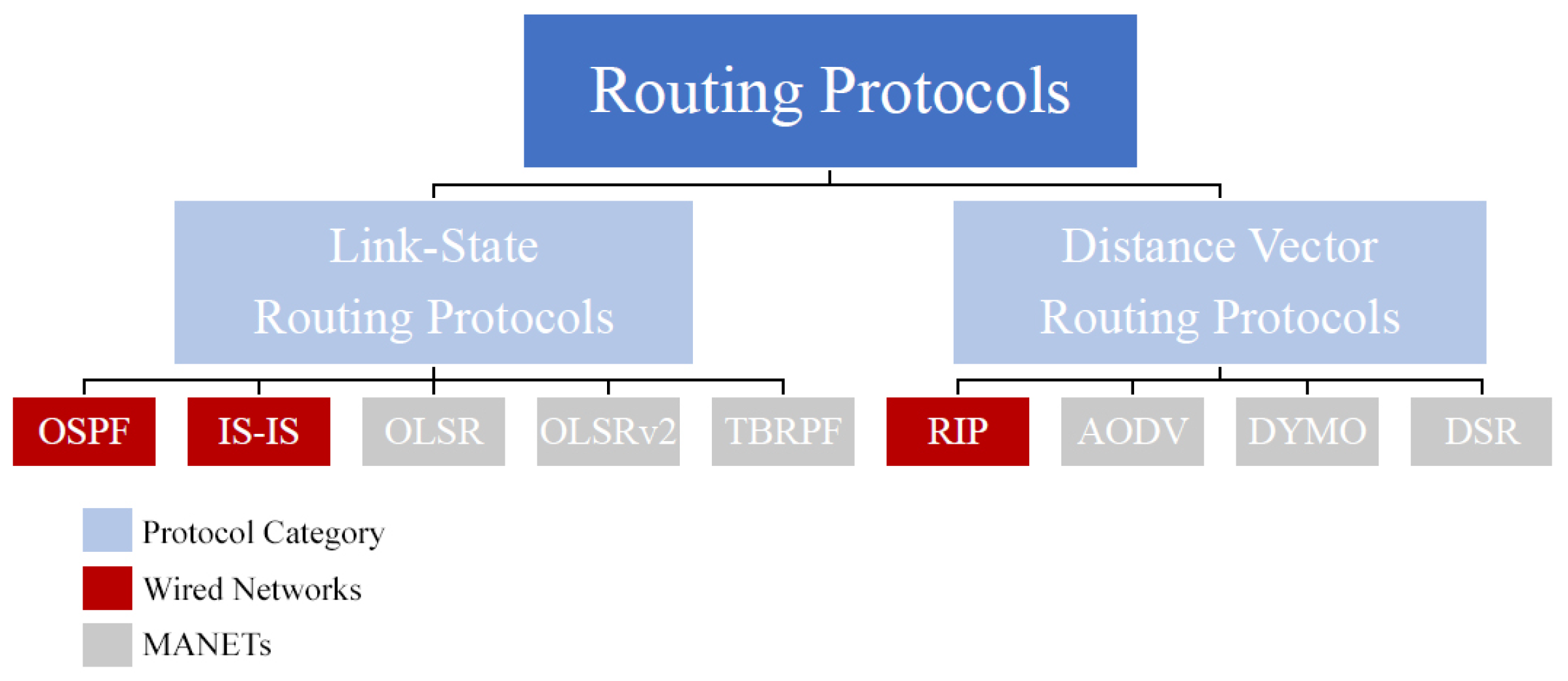
The most common LSRPs designed for wired networks are Open Shortest Path First (OSPF) [36,37,38] and Intermediate System–Intermediate System routing exchange protocol (IS-IS) [39,40]. OSPF allows the network to be divided into small areas, thereby creating a routing hierarchy. This hierarchy implies that a top-level routing area, i.e., the backbone area, connects other network areas. Routing information is exchanged through a group of nodes known as an Autonomous System (AS). The routing in AS takes place on two levels, intra-area and inter-area, depending on the position of the source and destination nodes. If the source and destination are in the same area, then intra-area routing is used, and if they are positioned in different areas, then inter-area routing is used.

Moreover, each node periodically sends “Hello” messages to establish a neighbour relationship. The shortest path to the destination is then calculated using the Dijkstra algorithm based on different link metrics such as link bandwidth and propagation delay. The information regarding the shortest distance to direct neighbours is stored in the neighbour table. In contrast, the routing information is stored in routing tables and updated when required. To store all of this information, i.e., neighbours and routing information, OSPF requires high CPU processing and consumes much memory. Moreover, the topology information of each area is hidden from the other areas in the network, and each area has its own LSDB [41]. Nodes belonging to the same area have an identical area LSDB, and nodes connected to multiple areas have separate LSDBs for each area. This isolation of routing information decreases control overhead and routing traffic caused by propagating the topology changes.

IS-IS was developed in 1987 by the International Organisation Standardisation (ISO) to provide routing for Open System Interconnect (OSI) environments [42,43]. In particular, IS-IS was designed explicitly to work with two ISO protocols: (i) Connection-Less Network Protocol (CLNP) [44] and (ii) End System to Intermediate System protocol (ES-IS) [45]. In IS-IS, the network is divided into routing domains that are divided into small areas. Each routing domain defines boundaries by setting some links as external links. Thus, routing messages in IS-IS are not transmitted through external links or exceed the domain boundaries. This division creates two-level routing hierarchies, Level 1 (L1) and Level 2 (L2), which are equivalent to the intra-area and inter-area in OSPF, respectively. L1 nodes, known as L1-ISs, have the topology map of their own area, and can only exchange routing information with other nodes in the same area. On the other hand, L2 nodes, i.e., L2-ISs, have the L2 topology and can exchange routing information and data packets directly with nodes from other routing domains. In some cases, a node can act as an L1-IS and L2-IS simultaneously, thus having the topology maps for both L1 and L2 domains. Separating the topology maps between levels decreases control overhead and routing traffic, which may be caused by propagating the topology changes through the network.

IS-IS periodically sends “Hello” messages for neighbour discovery to establish a neighbour adjacency. Topology information is then exchanged in the form of a Link-State Packet (LSP) within the area using the flooding technique. Each IS builds an LSDB based on the information received from the LSPs. A routing table is then created containing routing information regarding the best available paths between a source node and the neighbour nodes in the same area. Similar to OSPF, the best routing path is calculated using the Dijkstra algorithm based on different routing metrics, such as bandwidth and delay. Later, in 1990, the existing IS-IS was extended to support routing over the Transmission Control Protocol/Internet Protocol (TCP/IP) in addition to OSI [46]. The integrated IS-IS provides a single routing protocol that can efficiently perform over OSI, TCP/IP, and dual environments.

The most common LSRPs designed for MANETs are Optimised Link-State Routing (OLSR) [47,48], Optimised Link-State Routing version 2 (OLSRv2) [49,50], and Topology Dissemination Based on Reverse Path Forwarding (TBRPF) [51,52]. In OLSR, each node selects a set of direct neighbours known as Multi-Point Relays (MPR). In return, each MPR maintains a set of nodes that have chosen it to be an MPR called MPR selectors. These two sets are used to apply three optimisations: (i) only MPRs generate link-state information, (ii) only MPRs forward LSPs, and (iii) only MPRs advertise links connecting to its MPR selectors. In addition, OLSR establishes a new approach to minimise the number of flooding packets. This approach (i) imposes a time interval after each successful transmission of control packets and (ii) makes the triggered updates optional in case of topology changes. Compared with the traditional flooding technique, this new technique significantly reduces the number of control packets flooding through the network, thus reducing control overhead and bandwidth consumption [53]. OLSR calculates the best available path mainly based on hop counts. Hence, the shortest path between a source and destination node, with the minimum number of hops, is selected. Routing based on hop counts results in less changes in the formed routing paths, thus less updates and a more stable network.

However, shortest links in terms of minimum hop counts may not always be considered reliable paths. Minimum hop count links may lead to heavy use of long links in terms of the physical distance of these links [54]. For example, a source node may choose a long physical distance path with two hops to the destination over a shorter physical distance path with three hops. As a result, the long physical distance links may experience high (i) traffic load, (ii) bandwidth consumption, and (iii) packet loss; thus, lower PDRs occur. Therefore, in some situations, considering shorter physical distance links with extra hops may result in selecting more reliable paths with higher PDRs.

OLSRv2 is the successor of OLSR. It has the same functionality as OLSR with an enhanced ability to overcome the limitation in OLSR caused by using the hop count metric. OLSRv2 provides the ability to select the best path between source and destination nodes based on link metric rather than hop count. Another new feature of OLSRv2 is the use of MANET Neighborhood Discovery Protocol (NHDP) [55] for neighbour discovery. OLSRV2 exchanges “Hello” messages locally using the NHDP. By using NHDP, each node determines the presence of, and connectivity to, its 1-hop and 2-hop neighbours. The 1-hop information provides connectivity to direct neighbours, while the 2-hop information employs the flooding reduction technique.

TBRPF is another LSPR designed for MANETs. TBRPF consists of two main modules: (i) neighbour discovery module and (ii) routing module. The neighbour discovery model performs neighbour discovery using differential “Hello” messages that advertise only the changes in the neighbour status. Thus, the created “Hello” messages are smaller and sent more frequently. This allows TBRPF to detect topology changes and link failures faster than other LSRPs. In the routing module, each node maintains a source tree that provides the shortest paths to all reachable nodes in the network. The source tree is calculated using a modified version of Dijkstra’s algorithm based on partial topology information stored in the topology table. In addition, each node periodically advertises only a subset of its source tree to the neighbouring nodes. These partial advertisements help reduce the overall control overhead in TBRPF compared to other LSRPs. To ensure that all neighbours are updated with the advertised part of the source tree, i.e., subtree, TBRPF uses a combination of periodic and differential updates. Periodic updates advertise new neighbours of the subtree and ensure that each neighbour has information regarding the subtree, even if it does not receive all the updates. Differential updates ensure the fast propagation of each topology change to all nodes affected by the updates. Hence, each node advertises (i) periodic topology updates, e.g., every five seconds, and (ii) changes, such as adding or deleting to the subtree in more frequent differential updates, e.g., every two seconds.

Furthermore, TBRPF uses Reverse-Path Forwarding (RPF) [56] technique to flood LSU. RPF aims to establish loop-free forwarding of packets by forwarding packets in the reverse direction along the source tree. The received topology information is then used to compute the minimum hop count path between a pair of nodes in the source tree. Using RPF and minimum hop count in TBRPF instead of SPF results in more stable routing and less changes in the formed paths. Thus, less exchange of LSUs in comparison with other flooding techniques used in other LSRPs. In contrast, routing based on hop count only, without considering the link quality, may result in choosing unreliable paths with low bandwidth and PDRs. Therefore, TBRPF provides the option of selecting paths based on link metrics, e.g., signal strength, and selecting along paths with higher quality over minimum hop paths.

In general, the main advantage of LSRPs is the complete knowledge of the network topology, which allows nodes to find the shortest path to the destination quickly and efficiently. As well as recalculate the paths immediately in case of topology changes or link failures. In contrast, the two main disadvantages of LSRPs are (i) lack of scalability and (ii) excessive consumption of resources. The lack of scalability means that the routing protocol performance decreases with the increase in network size. This lack of scalability appears mainly as the number of nodes in the network increases, leading to an increase in advertisements and topology updates. Even though most LSRPs use triggered updates or partial updates, they often have high traffic loads as topology changes must propagate globally, which floods the network periodically with unnecessary packets. This flood tends to create excessive control overhead during path establishment. The more topology changes occur, the more advertisements are resent; thus, the higher control overhead and bandwidth consumption. Consequently, this type of routing is deemed unsuitable for (i) large networks or (ii) unstable networks with rapid topology changes.

Moreover, using an LSRP may impose high costs on the nodes. Each node has to (i) process packets, (ii) generate advertisement responses, and (iii) store massive amounts of topology and routing information. This results in excessive consumption of resources in terms of memory size, CPU processing, and power usage. Therefore, using an LSRP in a constrained network, such as LLN, that (i) often has nodes with very limited resources and (ii) suffers from rapid topology changes due to its Lossy channels, which may result in unstable performance with low PDR and high power consumption.

3.2. Distance Vector Routing Protocols (DVRPs)

The DVRP is a combination of the work proposed by Ford and Fulkerson [57] and Bellman [58]; it is referred to as the Ford–Fulkerson algorithm or the Bellman–Ford algorithm. In DVRP, the routing paths are advertised as vectors of distance and direction. Distance refers to the routing metric, whereas direction refers to the next hop. Each node maintains a routing table, i.e., Distance Vector Table (DVT), which contains the distance between the node itself and all its direct neighbours. In addition, nodes periodically advertise their entire routing table to all direct neighbours and rely on them to pass routing information to their neighbours as well. In this way, nodes learn about remote nodes in the network through second-hand information passed along by their direct neighbours. This is known as routing by rumour, whereby a node obtains information from a direct neighbour regarding remote nodes and accepts it without verifying its accuracy. This method is based on the assumption that the neighbour is trustworthy and has reliable information.

Furthermore, the received routing table entries are then combined with the existing entries. As a result, each node maintains and stores a complete routing table for the entire network. These routing tables are updated periodically. The best available path is calculated using the Bellman–Ford algorithm based on minimising the cost of each destination. The cost is mainly determined using the hop count metric. Thus, a source node selects the shortest path with minimum hop counts to a destination node. DVRP sends regular updates at a specified time interval, even if there are no changes in the network topology. This periodic update is a major source of routing information inconsistency and thus leads to a routing loop. Routing loops usually occur due to (i) link failure between a pair of nodes or (ii) two nodes sending routing updates simultaneously. Some DVRPs use the split horizon technique to overcome this problem by (i) preventing reverse route updates between two nodes and (ii) setting the maximum number of hops to 15.

The most common DVRP designed for wired networks is the Routing Information Protocol (RIP) [59,60,61,62]. The RIP is based on the Bellman–Ford algorithm that uses hop count as a routing metric to find the shortest path between a pair of nodes in terms of hops. Each node creates its own routing table that contains the routing information to all its direct neighbours. Then, it periodically advertises the entire content of the routing table to all direct neighbours. When a node receives an advertisement packet, it adds all entries to its routing table. This process ensures that every node has complete knowledge of all the paths in the network. A node can discover a link failure if it does not receive any advertisement packets from a direct neighbour for a long time. A directly connected neighbour has a hop count of 0, further nodes can be reached up to 15 hops, and any node after that, i.e., the 16th hop, is considered an unreachable node [63]. Hence, RIP is limited to networks whose longest path between a source node and a destination is 15 hops, which makes it unsuitable for large networks that require more than 15 hops to reach further destinations. Moreover, since RIP uses a fixed routing metric, i.e., hop counts, to select the best paths, it is often considered an appropriate metric in situations where paths need to be chosen based on real-time metrics, such as link quality metrics.

The most common DVRPs for MANETs are Ad-hoc On-Demand Vector (AODV) [64,65,66], Dynamic MANET On-Demand (DYMO) [67,68], and Dynamic Source Routing (DSR) [69,70]. AODV is an on-demand routing protocol in which a node searches for a path to another node only when the two nodes need to communicate. AODV uses the hop count metric; thus, the path with minimum hop counts between the source and destination is selected as the best available path. Other real-time metrics, such as link quality, are not considered, which may lead AODV to transmit packets over short but unreliable links. A source node initiates path discovery by flooding the network with route requests (RREQs) with an originator sequence number. The originator sequence number is used in path entry to point towards the source node that created the RREQ. When an RREQ reaches an intermediate node with a path leading to the destination, it sends route replies (RREPs) along the reverse path; otherwise, it retransmits the RREQ to its neighbours [71]. In the case of link failure, mainly owing to topology changes, AODV floods the network with (i) route errors (RERRs) to notify the affected nodes and (ii) new RREQs to find an alternative path. This technique allows nodes to find new paths to destinations immediately and efficiently during path discovery or link failure. Another feature of AODV is the use of the destination sequence number for each path entry. A destination node creates a destination sequence number to overcome Bellman–Ford limitation and ensure loop-free routing.

AODV uses bandwidth efficiently by minimising data traffic and control overhead compared to other DVRPs. It also reduces memory requirements by storing only the needed paths for active communications [72]. However, heavy traffic and control overhead may occur in two scenarios: (i) multiple RREPs may respond to a single RREQ and (ii) link failure where a large number of control packets are required to inform the affected nodes and find new paths. Moreover, AODV experiences a packet drop problem during link failure within active paths between a pair of nodes. This problem reduces efficiency in AODV as well as PDRs.

DYMO has been proposed as an evolution of AODV [64] and can be referred to as AODVv2. It has the same functionality as AODV, with simpler operations, different packet formats, and support for path accumulation. The DYMO operations are (i) path discovery and (ii) path maintenance. Path discovery operates at the source node to find a path to a new destination. In contrast, path maintenance operates to (i) avoid broken links in the routing table and (ii) reduce packet dropping in case of link failure in an active path. During these operations, DYMO uses the same routing messages as AODV, i.e., RREQs, RREPs, and RERRs. The path accumulation allows a single RREQ to create a path to all intermediate nodes forming this path without initiating RREQ themselves. As a result, path accumulation reduces traffic and control overhead in DYMO and packet loss owing to link failure compared to AODV. Although DYMO overcomes the limitation of packet drops in AODV, it still selects paths based on hop counts. Depending on hop count alone may lead to choosing the worst possible paths in many situations where real-time metrics should be considered.

DSR protocol is very similar to AODV as it searches for paths on-demand when a pair of nodes need to communicate with each other. The main difference is that DSR uses source routing instead of routing tables. Source routing allows the source node to select and control the path of its own packets. Each data packet carries the complete list of nodes forming a path to the destination in the header. By adding the source path to the packets header, intermediate nodes forwarding the packets can easily learn and use this routing information in the future. Source routing is a loop-free technique where source nodes determine each path, avoiding any inconsistency caused by using routing tables. As a result, DSR does not require sequence numbers or other techniques to prevent routing loops. DSR comprises two primary operations: (i) path discovery and (ii) path maintenance. Path discovery is used only when a source node attempts to send a packet to a new destination and does not have a path to reach it. Path maintenance is performed by a source node while using a source path to a destination to detect changes in the network topology, such as link failure. Both operations, path discovery and path maintenance, operate entirely on demand [73]. Therefore, unlike other protocols, DSR does not use any periodic routing advertisements, thus reducing traffic and control overheads. Path selection is based on hop counts, similar to other DVRPs, which repeat the possibility of routing over unreliable paths in terms of link quality.

The main advantage of DVRPs is routing based on local information received from direct neighbours rather than global knowledge of the entire network topology, such as LSRP. Hence, it significantly reduces overhead packets and bandwidth consumption compared to LSRP. In contrast, the main disadvantage of DVRPs is the disregard for link quality. Routing in DVRPs is mainly based on the minimum cost of distance, i.e., hop counts. It does not consider the link quality, an essential factor for Lossy channels as in LLNs, but not wired networks or hop-by-hop networks as MANETs for which these protocols are mainly designed. Therefore, using a DVRP in LLNs with a hop count metric only without taking into consideration the link quality may result in routing over unreliable paths with low PDRs.

3.3. Generic Routing Solutions vs. LLN Requirements

As generic routing protocols mentioned in Section 3 were not mainly designed for LLNs, there is a trade-off as these protocols may or may not meet the requirements of LLNs. Therefore, the IETF decided to evaluate these protocols against LLN requirements [74]. If an existing protocol meets these requirements, it can be used as a routing protocol for LLN, which would be very promising. Otherwise, a new protocol needs to be designed with all the requirements of LLN. The IETF has specified five criteria for a desirable routing protocol for LLN to compare the costs and benefits of the existing protocols in terms of these criteria. These criteria are (i) routing state, (ii) loss response, (iii) control cost, (iv) link cost, and (v) node cost.

The routing state reflects the ability to scale reasonably within the memory resources of LLN. Nodes often have very limited memory sizes for storing routing information, such as routing tables. Hence, routing protocols should take into consideration that nodes may be unable to store complete neighbour information. Therefore, it is important to ensure that the routing state scales with the size of the underlying network and within the memory constraints of a battery-powered node. As a result, a routing protocol that scales linearly with the network size fails to satisfy the routing state criterion. Loss response mainly illustrates how a routing protocol responds to link failures owing to loss of channel signal. A routing protocol that only propagates changes in an active path or to local neighbours passes this criterion. In contrast, a routing protocol that requires changes along any path to be propagated across the entire network fails in the loss response criterion.

Moreover, routing protocols require sending control packets for different tasks, such as detecting neighbours, discovering a topology, finding paths, or transmitting routing tables. The process of transmitting and receiving control packets, as well as data packets, costs nodes energy. In LLN, nodes often have limited power with low data rates. Routing protocols need to limit the transmission of control packets while conserving energy to minimise the network’s control overhead and energy consumption. By reducing these factors, routing protocols can significantly enhance network efficiency and longevity. Therefore, it is crucial to optimise routing protocols in terms of control packet transmission and energy consumption to ensure a highly efficient and long-lasting network. A routing protocol fails the control cost criterion if the transmission and receiving rates are not within the data rate limit. Link cost indicates the cost of finding a quality link. The quality of a link is measured using link quality metrics, and for each link, there is a cost associated with finding it. A routing protocol should be able to find the best available link with the minimum cost to pass this criterion. Node cost takes into account the node’s constraints, such as memory and power. A routing protocol that (i) considers these constraints when choosing the best path and (ii) can perform within the constraints of low memory and battery-powered nodes pass the node cost criterion. The IETF used these criteria to assess the routing protocols mentioned in Section 3.1 and Section 3.2, summarising the assessment results in

Table 2. Generic routing protocols assessment for LLNs.

Routing Category	Routing Protocol	Routing State	Loss Response	Control Cost	Link Cost	Node Cost
LSRPs	OSPF [36]	No	No	No	Yes	No
	IS-IS [39]	No	No	No	Yes	Yes
	OLSRv2 [49]	No	*	*	Yes	Yes
	TBRPF [51]	No	Yes	No	Yes	*
DVRPs	RIP [59]	Yes	No	Yes	*	No
	AODV [64]	Yes	No	Yes	No	No
	DYMO [67]	Yes	*	Yes	*	*
	DSR [69]	No	Yes	Yes	No	No

Yes: has satisfied the criterion; No: has not satisfied the criterion; *: need improvements.

[74] along with the symbols description.

As shown in Table 2, the first four protocols, LSRPs, passed the link cost criterion but failed or needed improvement to pass other criteria. LSRPs passed the link cost because these protocols take into consideration the link quality during path selection. In LSRPs, each node must learn the complete network topology map, which leads to large-size routing tables that scale linearly with the growth of network size. Therefore, LSPRs failed to satisfy the routing state criterion. The presence of routing information and topology changes in LSRPs can cause them to fail the control cost criterion. This is because this information needs to be propagated throughout the network, leading to an increase in control overheads. OLSRv2 [49] may have the potential to reduce control overhead to an acceptable level by using the Fisheye routing technique. However, there is no specification of how to accomplish the Fisheye technique; thus, OLSRv2 needs improvement in the control cost criterion.

OSPF and IS-IS require advertising and responding to any loss or changes in the link, i.e., link failure, even if the link is not actively used. As a result, OSPF and IS-IS failed to pass the loss response criterion. In contrast, OLSRv2 makes the triggered updates optional; thus, only some links’ changes are advertised. This raises a problem in topology consistency, as some links may fail but are not advertised through the network. Therefore, OLSRv2 received a “*” in the loss response criterion as it needs improvement. The TBRPF only advertises and responds to link failure in the active paths, so it passed the loss response criterion. OSPF does not consider other routing metrics related to the node itself, such as remaining energy or memory size, during path selection, and so fails the node cost criterion. On the other hand, IS-IS and OLSRv2 provide the option of using other node metrics besides the link metric and, therefore, pass the node cost criterion. TBRPF provides a way to use additional metrics, such as node metrics, but without a specification policy on how to use these additional metrics. Therefore, TBRPF received “*” on the node cost criterion as TBRPF needs improvement to pass this requirement.

The remaining protocols, DVRPs, satisfied the control cost criterion but failed most of the other criteria. RIP passed the control cost criterion because it uses triggered updates for advertising topology changes in active links. The remaining DVRPs are on-demand protocols where nodes generate control traffic only when they need to send data packets and pass the control cost criterion. A routing table of AODV and DYMO contains only the paths for communicating nodes in the network and thus passes the routing state criterion. RIP also passes the routing state criterion because, for each node, the routing table size can be scaled to the number of destinations instead of the number of nodes in the network. In contrast, even though DSR uses source routing, each node stores the source paths for all the destinations in addition to a blacklist of all unidirectional neighbour links; thus failing the routing state criterion. RIP and AODV propagate changes in the links even if they are not actively used and fail the loss response criterion. DYMO assessment shows some potential to meet the loss response criterion but requires precise specifications on how to meet the criterion while maintaining broken links. In contrast, DSR advertises unreachable destinations to the source node and passes the loss response criterion.

Moreover, AODV and DSR fail both link cost and node cost criteria because they only use the hop count metric for path-finding. RIP mainly uses the hop count metric but also provides the option of using other routing metrics. However, using real-time metrics such as link quality in RIP may lead to network instability; therefore, RIP needs additional implementations to pass the link cost criterion. In DYMO, the distance of a link can vary from 1 to 65535; thus, some improvements are required to use the link metric efficiently and pass the link cost criterion. Furthermore, DYMO may have the mechanisms to use node properties but also require additional implementations in order to use them properly and pass the node cost criterion. The remaining DVRPs do not support any node properties as a routing metric and thus fail the node cost criterion. It should be emphasised that none of the protocols, LSRPs or DVRPs, satisfy all the five criteria.

Table 3. Link-state Protocols vs. distance victor protocols.

Link-State Protocols	Distance Vector Protocols
Uses Dijkstra algorithm	Uses Bellman Ford algorithm
Based on link cost	Based on hop count
Triggered updates	Periodic updates
View whole network map	View from neighbour’s view
Send only the changes in the updates	Send entire routing table in the updates

summarises the general differences between LSRPs and DVRPs.

4. A Routing Protocol for LLNs (RPL)

Since none of the routing protocols mentioned in Section 3 meets the requirements of LLN, the IETF designed RPL [1] to provide routing services over IPv6 for LLN within the network and node constraints. This section reviews RPL and RPL routing solutions proposed recently. The solutions are then analysed against the reliable path requirements to identify knowledge gaps.

4.1. RPL Overview

An RPL [1] is explicitly designed to meet the requirements of LLNs, thus satisfying the five criteria mentioned in Section 3.3. Hence, RPL takes into account the limitations in terms of memory size, processing capability, and energy and performs within these constraints. RPL belongs to the DVRP category, which reduces the amount of topology information needed to perform the routing services compared to LSRPs. RPL organises the network topology as a Directed Acyclic Graph (DAG) oriented toward one or more nodes, i.e., DAG root, which acts as a sink. A DAG is divided into Destination-Oriented DAGs (DODAGs) per sink. The DODAG provides multiple forwarding paths towards the root via the so-called parent nodes. Each node in a DODAG selects a next hop node, i.e., parent node, to form a path connecting to the root node [75]. A set of one or more DODAGs creates an RPL Instance and shares the same unique identifier, RPLInstanceID. An example of an RPL Instance comprising two DODAGs with two different DODAG roots, R1 and R2, is shown in Figure 4.

To create and maintain DODAGs, RPL uses four types of control packets: (i) DODAG information object (DIO), (ii) DODAG information solicitation (DIS), (iii) destination advertisement object (DAO), and (iv) DAO acknowledgement (DAO-ACK) [76]. The four types of RPL control packets are illustrated in Figure 5. A DIS message allows new nodes to request DIO packets from neighbour nodes. A DIO message is considered the primary source of routing control information in an RPL. It contains essential information such as RPLInstanceID, node Rank, and routing metrics, which allows nodes to discover an RPL Instance, select a parent node, and maintain a DODAG. A DAO message is used to propagate destination information upward along the DODAG. Furthermore, nodes send a DAO-ACK as a response to receiving a DAO message. All RPL control packets are defined based on the Internet Control Message Protocol (ICMPv6) [77].

RPL provides a rank-based data-path technique to detect and repair loops when they occur in the network. This technique avoids routing loops by giving a rank for each node related to its position in the DODAG. As shown in Figure 6, a node with a high rank represents a far away node from the root, while a node with a low rank represents a close node to the root. Thus, packets are transmitted from the high-rank nodes toward the low-rank nodes until they reach the root. In other words, RPL does not prevent loops from happening but (i) tries to ensure that packets are transmitted forward to the root and (ii) triggers repairs as soon as possible when necessary [78]. In the case of link failure, RPL fixes links on-demand for the actively used links; thus, it reduces control overhead and avoids wasting energy in repairing unused paths [79]. Moreover, RPL uses an objective function to define how nodes select the best path toward the DODAG root within an RPL instance. The selection of parent nodes is based on different routing metrics, i.e., link and node metrics [80]. Thus, RPL separates packet processing and forwarding functions from the path-finding function. This separation of functions allows new objective functions to be plugged into RPL without altering other functions of RPL.

The IETF presents two main objective functions for RPL: (i) objective function zero (OF0) [81,82,83,84] and (ii) minimum rank with hysteresis objective function (MRHOF) [85,86,87]. Both of these objective functions are based on a single routing metric. OF0 uses the hop count as a routing metric to select the best parent from a set of neighbours in the DODAG. The hop count metric captures the number of hops, i.e., the number of relay nodes, involved in relaying or forwarding packets between a source and destination node. Usually, using hop counts as a routing metric provides stability to the network, as the shortest path in terms of hops often remains the same unless the node forming the path moves or runs out of battery. Another advantage of using the hop count is the simplicity of the metric, as computing and minimising the number of hops between a source node and a destination requires a simple addition.

However, the hop count metric only considers the number of hops for path selection. It does not consider the routing reliability issues caused by link quality or the node energy. Selecting the shortest path with minimum hop counts may lead to (i) routing over unreliable paths in terms of link quality and (ii) heavy use of long links in terms of physical distance. As a result, links may experience high traffic loads and bandwidth consumption, resulting in higher packet loss. In addition, relying on the same nodes to forward the packets over a long period imposes extra costs on the nodes, especially in terms of energy. This often leads to unbalanced use of energy resources around the network as nodes with low battery are chosen over nodes with full battery because they form the shortest path in terms of hop counts.

MRHOF uses the ETX routing metric for path selection. The ETX [88] is a link quality metric defined as the expected number of transmissions required to successfully transmit a packet through the link, including the retransmissions. Moreover, the total ETX of a path between a source and a destination is the sum of the ETX for each link forming this path. The ETX value of a link is calculated based on the links’ forward and reverse delivery ratios. Each node computes the ETX for the direct neighbours and selects the node with the minimum ETX value as a parent node. Thus, MRHOF allows nodes to find the minimum ETX paths to a root in the DODAG. The main advantage of using ETX as a routing metric is achieving a high throughput compared to the hop count metric [89].

In contrast, simplistically, using the ETX may not lead to selecting the most desirable paths. A path with the smallest ETX value may contain fewer hops with long physical distances or, in the worst-case scenario, a single long hop. This usually occurs as the path with more hops tends to have a higher ETX value, even if the links forming the path have better transmission rates. The decision to select paths with fewer hops of lower transmission rates may affect the network by (i) causing bottlenecks, in the case of a single long hop, and/or (ii) consuming more energy to reach the further apart nodes.

4.2. RPL Objective Functions for Non-Malicious LLNs

Over the years, multiple objective functions have been proposed to address the limitations of the main RPL objective functions, i.e., OF0 [81] and MRHOF [85]. The proposed objective functions differ in terms of (i) metrics used for path-finding optimisations and (ii) optimisation methods used for selecting the best path. The routing metrics can generally be divided into (i) link metrics and (ii) node metrics [80]. In contrast, the path-finding methods can be divided, based on existing objective functions, into (i) single metric method, (ii) combined metrics method, and (iii) fuzzy logic method. The existing objective function, as well as the main RPL objective functions mentioned in Section 4.1, can broadly be divided into groups based on the path-finding methods and the metrics used. The main objective functions [81,85] are discussed previously in Section 4.1, and the RPL objective function solutions for non-malicious LLNs are discussed in more detail below. The analysis of RPL objective functions for non-malicious LLNs is summarised in Table 4, while Table 5 provides a summary of the groups.

4.2.1. Single Metric Method

The first group of objective functions typically uses a single routing metric with a single metric method to select the best path. The single routing metric can belong to node or link metrics in this group. The objective function solutions with a node metric in this group include the OF0 [81], energy total consumed (ENTOT) [90], and energy-based objective function (Energy-OF) [91]. OF0 [81] selects the shortest paths in terms of hops. The latter two objective functions [90] and [91] are based on energy metrics, typically measured by the remaining node energy or energy consumption. Thus, the path with less energy cost is selected. In contrast, the objective function solutions that select the best paths based on a single link metric include the default MRHOF [85] discussed in Section 4.1, the average delay (AVG-DEL) [92], the received signal strength indicator-based (RSSI-based) solution [93], and the elaborated cross-layer RPL objective function (ELITE) [94].

Demicheli [90] proposed ENTOT, which uses energy consumption as a routing metric. ENTOT aims to balance the energy around the network by considering the energy consumption of each node along the path. The total energy consumption of a path is equal to the sum of the energy consumption of all the nodes forming this path. As a result, ENTOT selects the path with less energy consumption as the optimal path to reach the DODAG root. Simulation results show high performance for ENTOT in terms of energy consumption and network lifetime compared to MRHOF [85].

Kamgueu et al. [91] also proposed a similar idea to [90] and introduced Energy-OF. Energy-OF uses the node’s remaining energy as a routing metric. The Energy-OF aims to (i) prolong the network lifetime and (ii) distribute energy equally between the nodes by selecting the node with the highest remaining energy as a parent node. The Energy-OF approach uses a real-time battery level estimation model proposed in [95] to compute the node’s remaining energy. The battery model uses the current energy consumption of the node during each node state and its duration to estimate the node’s remaining energy. The experiments show that Energy-OF prolongs the network lifetime and distributes energy almost evenly between nodes, i.e., energy balanced, compared with MRHOF [85].

Although [90,91] reduce energy consumption and provide energy balance in RPL, they select routing paths based on the node’s energy level, which only addresses the routing reliability issues caused by power constraints and ignore other reliability issues that may cause by link quality.

Gonizzi et al. [92] proposed AVG_DEl to minimise the average delay towards the DODAG root. The AVG_DEL assumes that (i) the DAG root runs with a 100% duty cycle, and (ii) the nodes run with very low and different duty cycles, e.g., under 1%, at the media access control (MAC) layer [96]. The term duty cycle describes all forms of periodically switching off some functions, leaving them on only for a certain percentage of the time. In LLN, wireless radio transceivers often consume high power when they are switched on. Thus, nodes usually (i) switch off their radio transceivers as long as possible to save power and (ii) use a periodic wake-up to turn on their radio and listen for packet transmission. Nodes with long sleeping intervals cause longer delays compared to nodes with short sleeping intervals. The AVG_DEL results show a significant decrease in the end-to-end, mainly in the faraway nodes from the DAG root, i.e., leaf nodes, compared to MRHOF [85].

Lee et al. [93] proposed RSSI-based IPv6 that uses RSSI as a routing metric to improve the transmission performance in RPL. The RSSI-based IPv6 aims to (i) select stable links using the RSSI metric and (ii) dynamically change the length of IPv6 fragments. The RSSI metric estimates the packet loss rate in the links, while the dynamic fragmentation reduces the Frame Error Rate (FER) [97] in that link. This makes RSSI-based IPv6 more suitable for transmitting long IPv6 packets in RPL. The experimental results show that RSSI-based IPv6 reduces both FER and transmission time, thus improving the transmission performance.

Safaei et al. [94] proposed ELITE that introduces a new routing metric known as Strobe per Packet Ratio (SPR). SPR measures the number of transmitted strobes per packet in the MAC layer. ELITE prioritises paths that minimise strobe transmissions, thereby reducing overall transmission activity from source nodes to their destinations. Simulation results from ELITE indicate up to 25% reduction in average SPR and up to 39% improvement in node energy consumption compared to MRHOF [85].

However, [92,93,94] are based on link quality metrics, which only capture routing reliability issues as caused by channel errors or delays and do not address other routing reliability issues related to the node metric, such as the node’s energy.

4.2.2. Combined Metrics Method

The second group of objective functions uses combined routing metrics with a combined metrics method to select the best path. The combined routing metrics in this group can belong to either (i) the same metric category or (ii) different metric categories. This group consists of weighted random forward RPL (WRF-RPL) [98], congestion-aware objective function (CA-OF) [99], queue-utilisation-based RPL (QU-RPL) [100], congestion-aware Q-learning (CAQL) [101], PER-HOP ETX [54], expected lifetime (ELT) [102], lifetime and latency aggregatable metric (L2AM) [103], improved RPL (I-RPL) [104], and coordinator-based RPL (CB-RPL) [105].

Acevedo et al. [98] proposed WRF-RPL, an objective function designed for sensor networks with high traffic loads. WRF-RPL leverages remaining energy and the number of candidate parents as routing metrics to optimise load balancing. Simulation results demonstrate that WRF-RPL surpasses MRHOF [85] in terms of prolonging network lifetime and reducing control overheads. However, it is worth noting that WRF-RPL primarily focuses on remaining energy. It does not address reliability issues caused by link quality.

Al-Kashoash et al. [99] proposed the CA-OF, which uses buffer occupancy (BO) to avoid congestion in RPL. CA-OF concludes that, in high network traffic, most packets lost are caused by the buffer overflow. Therefore, CA-OF takes into account BO to reduce the number of lost packets in the buffer when congestion occurs. The proposed CA-OF combines two routing metrics: (i) BO for packet loss owing to buffer overflow and (ii) ETX for packet loss due to Lossy channels. Each metric has a weight of w corresponding to the buffer-free space and buffer occupancy as w1 and w2, respectively. The weight w1 is associated with ETX, whereas w2 is associated with BO. With low traffic and an empty buffer, w1 becomes 100%; thus, CA-OF selects paths mainly based on ETX. In contrast, with high traffic and a full buffer, w2 becomes 100%; hence, CA-OF selects paths mainly based on BO. As a result, the proposed CA-OF is aware of channel congestion and can forward packets through the least congested links. The simulation results show that CA-OF improves RPL performance in terms of throughput and PDR.

A similar idea as in [99] is proposed by Kim et al. [100] to minimise congestion under high traffic in RPL. The author investigates RPL in high-traffic networks and finds that most packet loss is caused by congestion. Hence, the author proposed QU-RPL to overcome the congestion problem and balance the load between nodes. QU-RPL take into consideration three routing metrics: (i) queue utilisation (QU), (ii) hop count, and (iii) ETX to select the best available path. The QU can be calculated as the number of packets in the queue divided by the total queue size. The experiment results show that QU-RPL balances the load effectively over the nodes and reduces the queue losses, thus increasing PDR.

Ahmed et al. [101] introduced CAQL, which incorporates congestion levels and ETX as routing metrics. CAQL employs a queue learning model based on reinforcement learning to mitigate network congestion and achieve load balancing. Simulation outcomes demonstrate CAQL’s positive impact on PDR, delay reduction, and energy consumption compared to related work.

The objective functions [99,100,101] combine different link metrics to overcome the packet loss limitation caused by congestion. Even though these objective functions improve (i) the routing reliability of packet delivery and (ii) balance the load between nodes, they have a common drawback: they only combine link metrics and do not consider any node metrics that may also affect routing reliability, such as node energy.

Xiao et al. [54] proposed PER-HOP ETX to overcome the long single-hop problem in RPL main objective functions [81,85]. PER-HOP ETX takes into consideration ETX and hop counts to calculate the average ETX value. Hence, the ETX value of each node in the path is distributed by dividing the sum of ETX by the hop count. Simulation results show that PER-HOP ETX selects better paths with high PDR and low latency compared to MRHOF [85] and OF0 [81]. Although PER-HOP ETX combines a link metric, i.e., ETX, and a node metric, i.e., hop count, it does not take into consideration the routing reliability issues caused by power constraints.

Iova et al. [102] proposed ELT, an energy-balancing objective function that distributes energy consumption evenly among nodes to improve network lifetime. This objective function uses the ELT routing metric to estimate the time until a node’s energy is depleted, i.e., residual time. The ELT metric is computed based on (i) forwarding traffic, (ii) ETX, (iii) energy drained, and (iv) residual energy. Thus, the path with the least energy constraint is selected as the best path to the DODAG root. Moreover, ELT provides two additional mechanisms to enhance RPL performance. The first mechanism allows for the detection of energy-bottleneck nodes and distributes traffic load evenly between the nodes. The second one allows nodes to select multiple preferred parents rather than just a single parent, as in the original RPL [1], to reduce maintenance costs in case of link failure. The experimental results show that ELT prolongs the network lifetime, avoids bottlenecks, and maintains a stable set of active parents.

Capone et al. [103] proposed L2AM that takes into consideration link quality and energy consumption. L2AM aims to balance energy by considering energy consumption so that each node consumes the same amount of energy. Therefore, the author proposed an Exponential Lifetime Cost (ELC) routing metric that takes into account (i) transmission power on the link and (ii) node residual energy. The ELC is then combined with the ETX metric in such a way that the weight of residual energy increases exponentially as the residual battery capacity decreases. Simulation results demonstrate that L2AM selects parent nodes with high energy, prolonging the network lifetime without affecting link reliability.

Cao and Yuan [104] proposed a new objective function called I-RPL. This objective function utilises five different routing metrics, which include the child number of a parent, candidate parent number, hop count, ETX, and energy consumption. I-RPL improves the calculation of path ETX to avoid selecting paths with long single-hop links. The simulation results indicate that I-RPL outperforms OF0 [81] and MRHOF [85] in terms of PDR, end-to-end delay, and energy consumption.

Ghosh and Chand [105] proposed CB-RPL that combines three routing metrics: ETX, hop count, and remaining energy. This objective function incorporates coordinator nodes responsible for handling control packets in the network. The coordinator nodes help to reduce network traffic and conserve energy by optimising control packet transmissions. The simulation results demonstrate that CB-RPL performs better than MRHOF [85] and OF0 [81] in various performance metrics such as PDR, delay, energy consumption, and throughput.

Although the objective function solutions [102,103,104,105] combine link quality and node’s energy metrics for path selection, they do not consider the issue of how to make global, i.e., end-to-end, optimum decisions for path selection in real time.

4.2.3. Fuzzy Logic Method

The third group uses combined routing metrics based on fuzzy logic methods. Zadeh first introduced fuzzy logic in [106] as a framework that can deal with uncertainty and approximation inputs. Unlike traditional logic based on binary true/false values, fuzzy logic allows for representing partial truth or partial membership in a set. In other words, it allows for a degree of “fuzziness” in the way of reason about things. Therefore, fuzzy logic is often used to solve problems that involve decision-making in uncertain or imprecise situations, resulting in making accurate and efficient decisions as possible [107]. As shown in Figure 7, fuzzy logic consists of four main components:

• Fuzzification—the process of converting specific input values into a certain degree of fuzzy set membership.
• Fuzzy rules/knowledge base—the if–then rules to follow are often derived from human expert opinions.
• Inference engine—the way of obtaining the final fuzzy conclusion based on the degree of membership of the input variables to fuzzy sets and detailed fuzzy rules.
• Defuzzification—the process of converting the fuzzy conclusions into detailed output values.

Similar to the second group, the combined routing metrics in fuzzy logic can belong to one or both of the metric categories. These objective functions include composite metric objective function (CMOF) [108], fuzzy-based mobility objective function (FMOF) [109], fuzzy analytic hierarchy process objective function (FAHP-OF) [110], optimisation fuzzy link quality estimation-based routing metric (Opt-FLQE) [111], objective function-based fuzzy (OF-Fuzzy) [112], objective function-based fuzzy logic (OF-FL) [113], objective function energy consumption (OF-EC) [114], and fuzzy logic-based objective function (FLEOF) [115].

Harshavardhana et al. [108] proposed CMOF, a fuzzy logic-based objective function that combines ETX with latency. CMOF addresses the problem of reliability and latency requirements during path selection. The latency metric is measured by the time a packet spends in the transmit queue plus the time it takes to access the channel. By considering ETX and latency as routing metrics, CMOF can select paths with less congestion and good link quality. The following fuzzy rule characterises the highest quality of a link: IF the link has a high ETX value AND low latency, THEN it has high quality. Simulation results show improvement in terms of PDR and latency compared to MRHOF [85].

Urama et al. [109] proposed FMOF, a fuzzy logic method that takes into consideration three routing metrics for path selection. The chosen routing metrics are (i) ETX to measure link quality, (ii) hop count to find the shortest path in terms of the hop, and (iii) RSSI to measure the received signal power. The following fuzzy rule obtains the quality of a link: IF the ETX value is small AND hop count is near AND RSSI is connected, THEN the link is excellent. Simulation results show that FMOF enhances the network performance in terms of PDR, average delay, and control overhead compared to MRHOF [85] and OF0 [81].

Koosha et al. [110] proposed FAHP-OF. This objective function harnesses fuzzy logic for soft-boundary decision-making and employs the Analytic Hierarchy Process (AHP) to combine multiple routing metrics. FAHP considers three routing metrics: ETX, RSSI, and hop count. The selected routing metrics for FAHP-OF are ETX, RSSI, and hop count. AHP uses a scale method table, which matches linguistic importance intensities to numerical numbers. Simulation results show that FAHP-OF maximises network performance in terms of PDR and network lifetime.

A similar idea, as in [108,109,110], is also proposed by Rekik et al. [111], who suggested combining four-link quality estimators as routing metrics using the fuzzy logic method. The proposed OF, namely Opt-FLQE, aims to improve RPL performance in smart grid environments and overcome the limitations of ETX in terms of (i) reliability, (ii) stability, and (iii) reactivity. These terms refer to (i) the ability to capture the real behaviour of a link, (ii) the ability to tolerate transient (short-term) degradation in link quality mainly due to environmental factors, e.g., noise or obstacles, and (iii) the ability to react quickly to persistent changes in link quality, respectively. The combined metrics are (i) smoothened packet reception ratio (SPRR), (ii) smoothened required number of packet retransmissions (SRNPs), (iii) average signal-to-noise ratio (ASNR), and (iv) link asymmetry level (ASL). These metrics measure packet delivery, packet retransmission, channel quality, and link asymmetry, respectively. The fuzzy rule that expresses the goodness of a link in Opt-FLQE is as follows: IF a link has high packet delivery AND low asymmetry AND low packet retransmissions AND high channel quality, THEN it has high quality. The obtained results show that Opt-FLQE is more reliable, stable, and reactive than MRHOF [85]. Thus, improving performance in terms of PLS and delay, specifically in smart grid environments.

The main drawback of these objective functions [108,109,110,111] is the absence of energy metrics, such as remaining energy among the combined metrics, as most of the routing metrics used in [108,109,111] are link metrics. Link quality metrics only capture routing reliability issues as caused by channel errors and do not address other routing reliability issues, such as nodes remaining energy and energy consumption.

Kamgueu et al. [112] proposed OF-Fuzzy, which takes into account both link and node metrics. OF-Fuzzy combines the following routing metrics: (i) ETX for link quality, (ii) delay to minimise the time a packet spends to reach the destination, and (iii) node’s remaining energy to prolong the network lifetime. OF-Fuzzy performs the fuzzification process over two phases to avoid the complexity of combining the three routing metrics directly. In the first phase, ETX and delay are combined to compute link quality where the following fuzzy rule gives the best link quality: IF ETX value is small AND delay is short, THEN the link quality is very fast. In the second phase, the quality value is combined with the remaining energy, and the fuzzy rule that expresses the goodness of a link is as follows: IF the quality value is very fast AND the remaining energy is full, THEN the link is excellent. Experimental results show that OF-Fuzzy has lower PLR, delay, and energy consumption compared to MRHOF [85]. Therefore, it improves the routing reliability and prolongs the network lifetime.

Gaddour et al. [113] proposed OF-FL that takes into consideration four routing metrics, namely ETX, end-to-end delay, hop count, and node’s remaining energy for path selection. The fuzzy rule expresses the goodness of a link in OF-FL can be defined as follows: IF the number of hop count is low AND end-to-end delay is low AND nodes remaining energy is high AND ETX value is small, THEN the link has an excellent quality. The OF-FL performance shows improvement in terms of end-to-end delay, network lifetime, and packet loss ratio compared with the performance of MRHOF [85] and OF0 [81].

A similar idea as in [112,113] is also proposed by Lamaazi and Benamar [114], who introduced the OF-EC. OF-EC considers both link and node metrics, i.e., ETX and energy consumption, for path selection. The energy consumption metric is adopted from ENTOT [90] and combined with ETX using the fuzzy logic method. Moreover, the hop count metric has been used in OF-EC to redirect packet transmission toward the root. The following fuzzy rule gives the quality of a link: IF ETX value is short AND energy consumption is low, THEN the link quality is very good. The obtained results show that OF-EC improves the network performance in terms of PDR, network lifetime, and energy consumption.

Soni et al. [115] proposed FLEOF that uses a Fuzzy Inference System (FIS) to combine three routing metrics: ETX, energy consumption, and hop count. FLEOF aims to address the limitations of RPL’s main objective functions, OF0 and MRHOF. Although FLEOF shows promise, it is still at the conceptual stage and has not been implemented yet. Future research will focus on conducting extensive simulation evaluations to determine FLEOF’s effectiveness compared to other related works.

These fuzzy logic solutions [112,113,114,115] take into account link and node metrics to improve routing reliability, in addition to making global optimum decisions for path selection. However, the main drawback of the fuzzy logic method is the complete dependence on human knowledge and expertise [116,117]. Fuzzy logic relies heavily on human knowledge and expertise to determine the membership functions and fuzzy rules. This can lead to bias and subjectivity in the decision-making process. For example, the author of OF-Fuzzy [112] considers the ETX value small if it is three or less, while any ETX value of 12 or bigger is considered a high value and builds the fuzzy rules based on these considerations. In contrast, the author of OF-FL [113] considers the ETX value small if it is ten or less, and if it is 80 or more, it counts as a high value of ETX. Furthermore, a set of fuzzy rules has been built based on these given values.

Table 4. Analysis of RPL objective functions for non-malicious LLNs.

Optimisation Method	RPL Objective Functions	R1	R2	R3	R4	R5
Single Metric Method	OF0 [81]	✗	✗	✗	✗	✗
	ENTOT [90]	✗	✓	✗	✗	✗
	Energy-OF [91]	✗	✓	✗	✗	✗
	MRHOF [85]	✓	✗	✗	✗	✗
	AVG_Del [92]	✓	✗	✗	✗	✗
	RSSI-based IPv6 [93]	✓	✗	✗	✗	✗
	ELITE [94]	✓	✗	✗	✗	✗
Combined Metrics Method	WRF-RPL [98]	✗	✓	✗	✗	✗
	CA-OF [99]	✓	✗	✗	✗	✗
	QU-RPL [100]	✓	✗	✗	✗	✗
	CAQL [101]	✓	✗	✗	✗	✗
	PER-HOP ETX [54]	✓	✗	✗	✗	✗
	ELT [102]	✓	✓	✗	✗	✗
	L2AM [103]	✓	✓	✗	✗	✗
	I-RPL [104]	✓	✓	✗	✗	✗
	CB-RPL [105]	✓	✓	✗	✗	✗
Fuzzy Logic Method	CMOF [108]	✓	✗	✓	❍	✗
	FMOF [109]	✓	✗	✓	❍	✗
	FAHP-OF [110]	✓	✗	✓	❍	✗
	Opt-FLQE [111]	✓	✗	✓	❍	✗
	OF-Fuzzy [112]	✓	✓	✓	❍	✗
	OF-FL [113]	✓	✓	✓	❍	✗
	OF-EC [114]	✓	✓	✓	❍	✗
	FLEOF [115]	✓	✓	✓	❍	✗

✓—considered; ✗—not considered; ❍—can be improved; R1—link quality; R2—energy level; R3—use optimisation method to make global optimum decision; R4—dynamic adaptation to network changes in terms of topology, link quality, and energy levels; R5—malicious threats.

Table 4. Analysis of RPL objective functions for non-malicious LLNs.

Optimisation Method	RPL Objective Functions	R1	R2	R3	R4	R5
Single Metric Method	OF0 [81]	✗	✗	✗	✗	✗
	ENTOT [90]	✗	✓	✗	✗	✗
	Energy-OF [91]	✗	✓	✗	✗	✗
	MRHOF [85]	✓	✗	✗	✗	✗
	AVG_Del [92]	✓	✗	✗	✗	✗
	RSSI-based IPv6 [93]	✓	✗	✗	✗	✗
	ELITE [94]	✓	✗	✗	✗	✗
Combined Metrics Method	WRF-RPL [98]	✗	✓	✗	✗	✗
	CA-OF [99]	✓	✗	✗	✗	✗
	QU-RPL [100]	✓	✗	✗	✗	✗
	CAQL [101]	✓	✗	✗	✗	✗
	PER-HOP ETX [54]	✓	✗	✗	✗	✗
	ELT [102]	✓	✓	✗	✗	✗
	L2AM [103]	✓	✓	✗	✗	✗
	I-RPL [104]	✓	✓	✗	✗	✗
	CB-RPL [105]	✓	✓	✗	✗	✗
Fuzzy Logic Method	CMOF [108]	✓	✗	✓	❍	✗
	FMOF [109]	✓	✗	✓	❍	✗
	FAHP-OF [110]	✓	✗	✓	❍	✗
	Opt-FLQE [111]	✓	✗	✓	❍	✗
	OF-Fuzzy [112]	✓	✓	✓	❍	✗
	OF-FL [113]	✓	✓	✓	❍	✗
	OF-EC [114]	✓	✓	✓	❍	✗
	FLEOF [115]	✓	✓	✓	❍	✗

✓—considered; ✗—not considered; ❍—can be improved; R1—link quality; R2—energy level; R3—use optimisation method to make global optimum decision; R4—dynamic adaptation to network changes in terms of topology, link quality, and energy levels; R5—malicious threats.

Table 5. Categories of RPL objective functions for non-malicious LLNs and the used metrics.

Optimisation Method	RPL Objective Functions	Routing Metrics	Metrics Category
Single Metric Method (Group 1)	OF0 [81]	Hop Count	Node Metric
	ENTOT [90]	Energy Consumption	Node Metric
	Energy-OF [91]	Node’s Remaining Energy	Node Metric
	MRHOF [85]	ETX	Link Metric
	AVG-DEL [92]	Average Delay	Link Metric
	RSSI-based IPv6 [93]	RSSI	Link Metric
	ELITE [94]	SPR	Link Metric
Combined Metrics Method (Group 2)	WRF-RPL [98]	Remaining Energy and Parent No.	Node Metric
	CA-OF [99]	ETX and Buffer Occupancy	Link Metrics
	QU-RPL [100]	ETX, Hop Count, and Queue Utilisation	Both
	CAQL [101]	Congestion Level and ETX	Link Metrics
	PER-HOP ETX [54]	ETX and Hop Count	Both
	ELT [102]	ETX, Forwarding Traffic, Energy Drained, and Residual Energy	Both
	L2AM [103]	ETX and ELC	Both
	I-RPL [104]	Child No., Parent No., Hop Count, ETX, and Energy Consumption	Both
	CB-RPL [105]	ETX, Hop Count, and Remaining Energy	Both
Fuzzy Logic Method (Group 3)	CMOF [108]	ETX and Latency	Link Metrics
	FMOF [109]	ETX, Hop Count, and RSSI	Both
	FAHP-OF [110]	ETX, Hop Count, and RSSI	Both
	OPT-FLQE [111]	SPRR, SRNP, ASNR, and ASL	Link Metrics
	OF-Fuzzy [112]	ETX, Delay, and Node’s Remaining Energy	Both
	OF-FL [113]	ETX, Delay, Hop Count, and Node’s Remaining Energy	Both
	OF-EC [114]	ETX and Energy Consumption	Both
	FLEOF [115]	ETX, Energy Consumption, and Hop Count	Both

Table 5. Categories of RPL objective functions for non-malicious LLNs and the used metrics.

Optimisation Method	RPL Objective Functions	Routing Metrics	Metrics Category
Single Metric Method (Group 1)	OF0 [81]	Hop Count	Node Metric
	ENTOT [90]	Energy Consumption	Node Metric
	Energy-OF [91]	Node’s Remaining Energy	Node Metric
	MRHOF [85]	ETX	Link Metric
	AVG-DEL [92]	Average Delay	Link Metric
	RSSI-based IPv6 [93]	RSSI	Link Metric
	ELITE [94]	SPR	Link Metric
Combined Metrics Method (Group 2)	WRF-RPL [98]	Remaining Energy and Parent No.	Node Metric
	CA-OF [99]	ETX and Buffer Occupancy	Link Metrics
	QU-RPL [100]	ETX, Hop Count, and Queue Utilisation	Both
	CAQL [101]	Congestion Level and ETX	Link Metrics
	PER-HOP ETX [54]	ETX and Hop Count	Both
	ELT [102]	ETX, Forwarding Traffic, Energy Drained, and Residual Energy	Both
	L2AM [103]	ETX and ELC	Both
	I-RPL [104]	Child No., Parent No., Hop Count, ETX, and Energy Consumption	Both
	CB-RPL [105]	ETX, Hop Count, and Remaining Energy	Both
Fuzzy Logic Method (Group 3)	CMOF [108]	ETX and Latency	Link Metrics
	FMOF [109]	ETX, Hop Count, and RSSI	Both
	FAHP-OF [110]	ETX, Hop Count, and RSSI	Both
	OPT-FLQE [111]	SPRR, SRNP, ASNR, and ASL	Link Metrics
	OF-Fuzzy [112]	ETX, Delay, and Node’s Remaining Energy	Both
	OF-FL [113]	ETX, Delay, Hop Count, and Node’s Remaining Energy	Both
	OF-EC [114]	ETX and Energy Consumption	Both
	FLEOF [115]	ETX, Energy Consumption, and Hop Count	Both

Moreover, the fuzzy logic method is not flexible; it can only support the use of pre-defined rules, the if-then conditions, which makes the method only suitable for specific network scenarios and can not adapt to the network changes as human intervention may be required to update or specify new rules. For example, in OF-FL [113], the if-then rules have been set based on the following network scenario: an area of 600 × 600 m with 100 nodes. Thus, OF-FL considers a destination node with ten hop counts away from the source node as average hops compared to the area size and node density. However, in a different network scenario, e.g., 100 × 100 area with 20 nodes, ten hop counts are considered very far, while the average hop count may lie between three and five hops. Therefore, human intervention is needed to update the fuzzy rules and membership functions to obtain more accurate results for OF-FL in a smaller network area with lower node density.

It should be emphasised that, to the best of our knowledge, none of the existing RPL solutions mentioned in Section 4.2 take into consideration the reliability issues caused by malicious nodes.

4.3. RPL Objective Functions for Malicious LLNs (MLLNs)

Security threats, such as PDAs, can significantly impact the reliability of network routing by disrupting the normal flow of data packets between the source and destination. Available security solutions for wired and ad hoc networks may not be applicable to RPL due to nodes’ limited resources in terms of memory, CPU processing, and power. Multiple RPL security solutions have been proposed to (i) detect and avoid communication with malicious nodes and (ii) perform within the node constraints in LLNs.

Djedjig et al. [118] proposed the trusted RPL that secures RPL by adding a new trustworthiness metric called RPL Node Trustworthiness (RNT). Trust between nodes participating in routing is a very important factor in maintaining secure and reliable transmission. The new metric represents a trust level for each node in the network, which allows nodes to decide whether or not to trust their neighbour nodes as parent nodes during path selection. However, the proposed metric imposes high costs on the node resources; thus, it can not be applied to the constrained nodes in LLNs. As a result, all the security computations and processing have been offloaded into a small hardware device known as the Trusted Platform Module (TPM). The responsibilities of TPM include two main tasks: (i) ensuring secure cryptography and authentication methods during the transmission of control packets and (ii) performing computations and processing of nodes’ behaviours. Although this solution can secure RPL against security threats, it only takes into account the trust level of direct neighbours and does not consider the trust value along the selected path.

The latter drawback was overcome in [119], where Djedjig et al. proposed a trust-based metric, namely the Extended RPL Node Trustworthiness (ERNT), that takes into consideration the trust value of all the nodes forming the path. ERNT is a quantitative and dynamic metric that aims to enhance security in RPL by establishing a trust relationship between the nodes, allowing a node to decide whether or not to trust neighbour nodes in the network. Each node calculates (i) the trust value of its direct neighbour, i.e., first hop, and (ii) the total trust value of all the nodes forming the path. The proposed metric is then integrated into RPL with a new objective function known as the trust objective function (TOF). Owing to the node constraints, a hardware security chip has been embedded in each node to (i) provide authentication and cryptography for control packet transmission and (ii) offload the extra computations and processing for ERNT metric. Experimental results show that TOF has better performance in terms of node trust, leading to the selection of more secured paths compared to MRHOF [85].

However, both solutions [118,119] impose excessive costs on the nodes; thus, they require an impeded security chip as they can not be applied directly to the nodes. In addition, they only take into account the reliability issues caused by malicious nodes, and did not consider other reliability issues caused by the link quality or node energy.

Hassan et al. [120] proposed a security framework for RPL known as the Gini Index-Based Trust Mechanism (GITM). GITM uses a layered system as it separates the process of detecting the security attacks from the nodes in a separate layer. The fog layer is assumed to be reliable, secure, and trustworthy. In this layer, three main processes are performed. By adding a fog layer, nodes present in the network do not calculate trust in themselves. Because it consumes a significant amount of energy, network nodes can also be attacked and compromised, leading to security issues. Therefore, all the trust calculations are performed in the fog layer, which is fully trusted. Simulation results show that GITM significantly detects the attacks and improves detection rate, latency, and energy consumption.

Ahmadi and Javidan [121] proposed the Trust-based RPL Attacks Detection (TRAD) system, leveraging recurrent neural networks (RNNs) to enhance security. The system consists of four modules: (i) behaviour generation, (ii) sequence prediction, (iii) trust analysis, and (iv) attacker detection. The behaviour generation module generates behaviour profiles of sensor nodes during data transmission. The sequence prediction module predicts sequences of expected behaviour using the generated behaviour profiles. Trust analysis assesses the trust level of each node based on deviations from the expected behaviour during data traffic. In the attacker detection module, TRAD uses trust assessments to detect compromised nodes, specifically targeting two notorious RPL attacks: black-hole and grey-hole attacks. Although TRAD offers promising security enhancements, its main challenge lies in the training phase. This phase incurs significant computational overhead and must be conducted on edge sensor nodes, which adds to the complexity of implementation.

Karkazis et al. [122] proposed Packet Forwarding Indication (PFI), a trust-related metric that detects whether the selected parent has actually forwarded the packets. PFI can be defined as the probability that a packet will be successfully transmitted along a path without being dropped. This can be calculated as the number of successful forwarded packets divided by the total number of successful and unsuccessful forwarded packets for each node forming the path. The proposed metric, PFI, has been combined with the hop count metric, i.e., HCPFI, to select short paths and avoid malicious nodes. Experimental results show significant improvements in detecting malicious nodes; thus, better PDR and latency compared to OF0 [81]. Even though HCPFI takes into consideration both node and security metrics, it does not address the reliability issues caused by link quality or node energy.

To overcome some of the limitations of the previous solution [122], Karkazis et al. [123] proposed the Expected Frame Transmissions Packet Forwarding Indication (TXPFI) metric. TXPFI combines two routing metrics: (i) the PFI metric for node trust from [122] and (ii) the TX metric for link quality. The TX metric is similar to the ETX metric except that TX captures the expected number of frame transmissions instead of packets, including retransmissions needed to deliver data successfully. The author also proposed another combination of metrics for PFI with ETX and compared the performance of the two solutions, i.e., TXPFI and PFIETX, against each other. The obtained results prove TXPFI’s efficiency in avoiding malicious nodes and/or unstable links, but PFIETX performs best with the lowest PLR at the expense of long paths.

Thulasiraman and Wang [124] proposed a lightweight trust-based security architecture to select routing paths in RPL based on combined metrics. The metrics used are (i) the node trust to identify malicious nodes in the network and (ii) the average received signal strength indicator (ARSSI) for link quality. The node trust metric adopts a binary trust model that can avoid communication with malicious nodes and minimises the node trust computation at the same time. The simulation results showed better PDR performance than MRHOH [85] but with increased control overheads.

Although [123,124] address the reliability issues caused by malicious attacks and link quality, they do not consider the reliability issues caused by node metrics such as energy consumption or remaining energy.

Airehrour et al. [125] proposed another trust-based solution to secure RPL against PDAs without imposing extra control overheads. The proposed node trust metric provides a feedback-aware security system that computes a trust value for each node based on the forwarding behaviour of direct neighbours. The trust value is computed as the number of packets delivered through a neighbour node divided by the total number of packets sent to this neighbour node. The obtained results show that the node trust metric isolates malicious nodes from routing decisions and enhances throughput compared to MRHOF [85].

Airehrour et al. [126] improved the latter solution [125] and introduced the Secure Trust-aware RPL (SecTrust-RPL). The proposed solution computes trust based on successful packet transmission between nodes to determine their reliability in forwarding packets. SecTrust-RPL uses the following three metrics: (i) direct trust from [125], (ii) neighbour recommendation for trust computation, and (iii) trust aggregation. Direct trust measures the trustworthiness of direct neighbours, i.e., the first hop, while the neighbour recommendation measures trust towards the distant nodes of interest. The third metric, trust aggregation, measures a direct neighbour’s trust value at time t to compare it against a given threshold. Therefore, SecTrust-RPL can (i) detect and isolate malicious nodes and (ii) make adaptive changes related to environmental conditions due to node mobility. Simulation results prove the efficacy of SecTrust-RPL in isolating malicious nodes during path selection, which significantly reduces PLR compared to MRHOF [85].

A similar idea as in [126] is also proposed by Mehta and Parmar [127], who suggested a lightweight trust-based mechanism that uses direct and indirect trust metrics to address the security threats in RPL. Direct trust computes based on node properties for direct neighbours, i.e., first hops, while indirect trust computes for the second hop neighbours based on the opinion of the first hop neighbours. The calculation of the direct trust metric is the same as in [125]. Furthermore, the indirect trust metric multiplies the direct trust values of the first and second hops. The total trust value for each node is then represented as the sum of direct and indirect trust values. Simulation results show that the trust-based mechanism can detect and isolate malicious nodes, thus increasing throughput compared to MRHOF [85].

The main drawback in [125,126,127] is the fact that these solutions are mainly based on trust metrics, which only capture the reliability issues caused by malicious attacks and do not address other reliability issues, such as link quality and remaining energy. Moreover, to the best of our knowledge, none of the existing RPL security solutions mentioned in this section address the reliability issues properly by considering the most affected factors: (i) malicious attacks, (ii) link quality, and (iii) energy. The security solutions are analysed against the reliable path requirements to identify knowledge gaps. A summary of the analysis is given in

Table 6. Analysis of RPL objective function solutions for MLLNs.

RPL Objective Functions	R1	R2	R3	R4
Djedjig et al. [118]	✓	✗	✗	✗
Djedjig et al. [119]	✓	✗	✗	✗
Hassan et al. [120]	✓	✗	✗	✗
Ahmadi and Javidan [121]	✓	✗	✗	✗
Karkazis et al. [122]	✓	✗	✗	✓
Karkazis et al. [123]	✓	✓	✗	✓
Thulasiraman and Wang [124]	✓	✓	✗	✓
Airehrour et al. [125]	✓	✗	✗	✓
Airehrour et al. [126]	✓	✗	✗	✓
Mehta and Parmar [127]	✓	✗	✗	✓

✓—considered; ✗—not considered; R1—malicious threats; R2—link quality; R3—energy level; R4—perform within node constraints.

below.

5. Existing Surveys on RPL

Several surveys have explored routing solutions for LLNs, with a particular focus on RPL. These surveys have shed light on the core intricacies of RPL and its deployment across diverse environments, providing valuable insights into the unique characteristics and inherent limitations of the protocol. Although these efforts have significantly contributed to the understanding of RPL, there is still a need for further research. A comprehensive examination of existing RPL surveys, presented in

Table 7. Summary of existing surveys on RPL.

RPL Survay	Scope	Publication	Year
Ghaleb et al. [128]	RPL core operations and limitations particularly in areas such as efficient downward route construction, load balancing, and metric composition	IEEE Journal	2019
Kharrufa et al. [129]	RPL evaluation in various IoT applications based on enhancement areas and service types	IEEE Journal	2019
Kamgueu et al. [130]	RPL implementations and recent contributions related to topology optimisation, security, and mobility	Elsevier Journal	2018
Witwit and Idrees [131]	RPL implementation, performance, applications evaluation, and improvement	Springer Conference	2018
Aljarrah et al. [132]	RPL objective functions and their impact on RPL performance and key metrics used in the implementation of the objective function	IEEE Conference	2017
Kamble et al. [16]	Categorisation of attacks, prevention of topology attacks in RPL, and examines secure routing protocols within the IoT context	IEEE Conference	2017
Kim et al. [76]	History of research efforts in RPL, experiments conducted on real embedded devices, and RPL adoption in real-world systems and applications	IEEE Journal	2017
Zhao et al. [133]	RPL and P2P-RPL performance evaluations, research challenges, and potential opportunities	Springer Journal	2016
Pongle and Chavan [15]	Security aspects of RPL in the context of IoT, potential attacks, countermeasures to mitigate these attacks, and their consequences on network parameters	IEEE Conference	2015
Gaddour and Koubaa [134]	RPL architecture including performance evaluation, implementation, and enhancement of the RPL	Elsevier Journal	2012

, highlights two essential aspects that require more exploration. Firstly, routing metrics that impact delivery reliability and efficiency within RPL objective functions in LLNs and MLLNs need to be comprehensively explored. Secondly, further investigation is required into the path-finding methodology employed by RPL solutions, and their ability to make optimal decisions globally in real time while adapting to dynamic changes in the network. This underscores the need for a more thorough exploration of these aspects to provide a holistic understanding of reliability issues in RPL, encompassing various influencing factors and potential security threats in LLNs. Our survey aims to offer a detailed understanding of these crucial factors, including both malicious and non-malicious factors, providing valuable insights into RPL’s routing metrics and path-finding methods.

Ghaleb et al. [128] presented an in-depth survey and comparative analysis aiming to address the weaknesses of RPL. The discussion begins by providing an introduction to LLNs, their communication technologies, and the routing requirements based on the RPL standard. The survey intends to assess whether RPL extensions effectively overcome previously reported limitations related to its core operations, including objective functions, routing maintenance, and downward routing primitives. In conclusion, the survey underscores the need for further research efforts, particularly in addressing challenges hindering the adoption of the standard in large-scale deployments. The identified research directions aim to propel the understanding and improvement of RPL in real-world applications.

Kharrufa et al. [129] conducted a systematic review of RPL-based routing protocols, providing technical insights and evaluations of various RPL implementations and optimisation approaches found in the literature. The review assessed the current state of RPL, emphasising its growing interest and relevance in IoT applications. The analysis showed a shift in focus over the years, from early concerns about energy-saving improvements to later considerations of additional functionalities and core design enhancements. The authors recognised RPL as a widely accepted IoT routing protocol and highlighted research trends, including industrial applications, cross-layer design, and security-enabled RPL. The authors also proposed a more flexible framework to address features such as congestion control and mobility, fostering interoperability among various RPL adaptations documented in the literature.

Kamgueu et al. [130] focused on optimising the network topology in the context of RPL. They consider important factors such as the application goals, communication security, and node mobility within the network. To lay the groundwork for their exploration, the authors first revisit fundamental aspects of RPL. They then provide a comprehensive review of objective function implementations proposed to optimise the routing topology construction process. In addition, they uncover the principal threats prevalent in the RPL landscape and discuss proactive efforts and countermeasures devised to effectively mitigate these security challenges. The authors also highlight the dynamic nature of node mobility within RPL networks, emphasising the importance of considering mobility, and shedding light on the enhancements that have been made to the RPL framework to address the challenges associated with the movement of nodes.

Witwit and Idrees [131] provided a comprehensive exploration of the RPL routing protocol, addressing both foundational aspects and practical considerations with a specific emphasis on its applications in IoT and associated challenges. The survey is divided into two main sections. The initial part introduced the survey, reviewed the related literature, and delved into the scientific background and main features of the RPL routing protocol. The subsequent part shifted focus to the latest advancements in RPL research, navigated through challenges in RPL routing, particularly within the IoT landscape, and engaged in discussions while offering additional analysis. The critical role of RPL routing in IoT environments, which are characterised by unreliability and multi-hop interference, is emphasised. The survey also reviewed various routing protocols tailored for LLNs and outlined open research issues and future directions in the field.

Aljarrah et al. [132] presented a comprehensive review of the current and recent advancements in RPL. The focus extends to surveying existing approaches and protocols, aiming for a comparative analysis of the utilised objective functions. The paper summarised the characteristics of main routing metrics, facilitating a comparison that underscores the need for further research on the validity and effectiveness of existing metrics or the development of new ones. As part of future work, the authors proposed an investigation into RPL performance in high-density networks using two objective functions, namely MRHOF and OF0, in various topologies.

Kamble et al. [16] focused on examining the security aspects of LLNs in the context of the IoT. They emphasised the importance of identifying and analysing security attacks on RPL, which is crucial for enabling communication among IoT devices. The paper classified attacks into three main categories: attacks against resources, attacks against the topology, and attacks against network traffic. Attacks on resources involve actions that reduce the network lifetime, while attacks against the topology aim to manipulate the network configuration. Attacks on network traffic focus on capturing and analysing a significant portion of the traffic. The paper also discussed various techniques to protect RPL topologies and highlighted the critical role of secure routing in ensuring the seamless and safe functioning of IoT networks. Additionally, the authors emphasised the need for a universal solution that can be applied to all routing attacks, both present and future.

Kim et al. [76] provided a detailed analysis of RPL, focusing on its usage and evaluation in several published works. The survey finds that RPL has been extensively evaluated through both test-bed experiments and simulations in various application domains. Notably, many evaluations have used prototype implementations on real embedded devices, with ContikiOS and TinyOS being the most popular implementations. The results of the survey indicate that many optional RPL functionalities are not well-supported or necessary in many scenarios, which raises questions about their relevance and impact on the protocol’s simplicity and interoperability.

Zhao et al. [133] conducted a thorough study of the RPL and P2P-RPL protocols. Their study included a detailed evaluation of the routing performance of these protocols, addressing major research challenges, and categorising key research directions while introducing potential technological enhancements. The paper presented the routing specifications of RPL and outlined an implementation framework using NS-3. Experimental evaluations of RPL and P2P-RPL protocols have been conducted, providing insights into their performance. The paper also identified active research areas and challenges related to RPL and addressed these challenges with enabling techniques.

Pongle and Chavan [15] discussed the impact of attacks on RPL network parameters. They presented a survey of existing detection systems and focused on research areas for RPL attack solutions. The authors emphasised the need for research on countering RPL network attacks, particularly those that have not yet been evaluated. The authors proposed mechanisms to counter attacks such as Wormhole, Sybil, clone ID, and black-hole. They have expressed a need for the deployment of detection and prevention mechanisms that are based on detection systems or other suitable alternatives. The implementation of these mechanisms would contribute to a more secure system, ensuring the confidentiality and integrity of RPL.

Gaddour and Koubaa [134] conducted a detailed study of the design objectives and network architecture of RPL. They outline the protocol control headers, network construction operations, and network management mechanisms, including fault tolerance, quality of service (QoS), and security aspects. The researchers also perform an empirical analysis to evaluate the performance of RPL in practical settings. They investigate the impact of various RPL attributes on network behaviour and compare it with other routing protocols. This comparative analysis provides valuable insights into the strengths and potential areas of improvement for RPL.

6. Further Discussions

Based on the above critical analysis of related work, we observe that there is still room for improvements in the existing routing solutions to achieve reliable path-finding in LLNs. More specifically, we have made the following observations.

Firstly, none of the existing solutions designed for LLNs, i.e., RPL solutions, consider the most reliability-effecting factors, particularly node energy level and link quality during a path selection process using a path selection method that can make a global optimum decision based on multiple reliability-effecting factors in real time in adaptation to the network topology, link quality, and energy level changes. Considering these features during path-finding in LLNs may result in achieving reliable paths with high PDRs and extended network lifetime.

Secondly, existing routing solutions designed for LLNs assume that the main causes of reliability issues are non-malicious factors such as link quality and energy levels. None of the existing routing solutions explicitly addresses the issue of maximising PDR, considering the most reliability-effecting factors mentioned above, with the presence of malicious nodes. Detecting malicious behaviours, such as packet dropping, in LLNs is challenging using standard link quality metrics. Malicious nodes can appear legitimate when joining a network but engage in malicious activities during the packet forwarding stage, impacting packet delivery reliability.

Thirdly, even though there are multiple security solutions in the literature that can successfully measure the trustworthiness of participating nodes and isolate malicious nodes from communicating with other nodes in the network, they only consider the reliability issue caused by malicious nodes. To the best of our knowledge, none of the existing security solutions address (i) the reliability issues caused by multiple reliability-effecting factors, particularly energy levels, or (ii) how to make a global optimum decision in real time with adaptation to the network changes.

7. Conclusions

This paper presents our comprehensive research and investigation toward a reliable path-finding solution for LLNs in the presence of PDAs. It discusses the unique characteristics of LLNs and their impact on routing reliability and security. Followed by a critical analysis of the generic routing protocols and RPL objective functions in non-malicious and malicious LLNs. The existing solutions have been critically examined against the requirements for reliable path-finding and identifying areas for further improvements.

Our future work includes designing and implementing a reliable path-finding solution for LLNs with PDAs to improve delivery reliability and routing efficiency in LLNs.