A Multimodel-Based Approach for Estimating Cause of Scanning Failure and Delay in IoT Wireless Network ^†

Abstract

The rapid growth in the IoT network comes with a huge security threat. Network scanning is considered necessary to identify vulnerable IoT devices connected to IP networks. However, most existing network scanning tools or system do not consider the burden of scan packet traffic on the network, especially in the IoT network where resources are limited. It is necessary to know the status of the communication environment and the reason why network scanning failed. Therefore, this paper proposes a multimodel-based approach which can be utilized to estimate the cause of failure/delay of network scanning over wireless networks where a scan packet or its response may sometimes be dropped or delayed. Specifically, the factors that cause network scanning failure/delay were identified and categorized. Then, using a machine learning algorithm, we introduced a multimodel linear discriminant analysis (MM-LDA) to estimate the cause of scan failure/delay based on the results of network scanning. In addition, a one-to-many model and a training data filtering technique were adopted to ensure that the estimation error was drastically reduced. The goal of our proposed method was to correctly estimate the causes of scan failure/delay in IP-connected devices. The performance of the proposed method was evaluated using computer simulation assuming a cellular (LTE) network as the targeted IoT wireless network and using LTE-connected devices as the targeted IoT devices. The proposed MM-LDA correctly estimates the cause of failure/delay of the network scan at an average probability of 98% in various scenarios. In comparison to other conventional machine learning classifiers, the proposed MM-LDA outperforms various classification methods in the estimation of the cause of scan failure/delay.

1. Introduction

With a continuous growth of over 50 billion connected devices worldwide over the Internet [1], one of the most challenging problems is determining how to secure an IoT wireless network and devices that are connected to it. It is of concern that there may be many IoT devices deployed with their default settings that makes them vulnerable to cyberattacks. Such devices are used as a tool by attackers for carrying out distributed denial of service (DDoS) attacks [2], which often results in a large amount of unauthorized communications. Furthermore, there have been many cases of cyberattacks targeting vulnerable IoT wireless devices such as home thermostats, baby monitors, IP cameras, etc. For example, in 2017, an IoT botnet named “Persirai – ELF_PERSIRAI.A” targeted over 1000 different models of Internet Protocol (IP) cameras via an open port (TCP port 81). It was confirmed via Shodan that 120,000 IP cameras were detected as infected [3]. Therefore, “wide-area-network scanning” techniques are necessary to detect compromised IoT wireless devices and provide adequate countermeasures against such threats in an IoT network.

However, when network scans are performed, the status of the scanned device port is reported as “open”, “closed”, or “filtered/blocked”. The problem is that when a network scanning fails to acquire a response from a particular port of a device, the status may be considered as “filtered/blocked” and the reason for such failure (i.e., a failure that occurred because of bad network condition) is not considered. It is possible that a device whose ports are considered as safe, due to the “filtered/blocked” status reported during a bad network condition, may be vulnerable to a cyberattack if the ports are actually open. One possible solution to confirm the real status of the scanned port is to perform a rescan. However, if the port is actually closed, the traffic during the rescanning can interfere with the regular communication of the network, especially in a resource-constrained IoT wireless network. Therefore, in order to perform a network scan reliably and efficiently, it is necessary to know the condition of the network, and whether it is good or not for performing a network scan. Moreover, it is essential to determine the cause of network scan failure/delay [4] in relation to the communication environment status for appropriately scheduling a network scan. Hence, a technique for determining and estimating the cause of network scan failure/delay is required.

In this paper, we propose a multimodel-based approach which can be utilized to estimate the cause of failure/delay of the network scan over wireless networks where a scan packet or its response may sometimes be dropped or delayed. Specifically, various factors that cause network scanning failure/delay are identified and categorized based on the network status. Furthermore, we utilize machine learning algorithms to estimate the cause of failure/delay based on the results of a series of network scanning obtained under various network scenarios (i.e., normal, low signal-to-noise-ratio, and network congestion). Herein, we modify the operation of the conventional linear discriminant analysis (LDA) by generating a multimodel linear discriminant analysis (MM-LDA) based on two discriminant functions. In addition, a one-to-many model approach is applied to the scan data to reduce the estimation error of the scan failure/delay where the scan response samples obtained in various network scenarios overlapped. The goal of our proposed method is to correctly estimate the causes of scan failure/delay in IP-connected devices. The main contributions of this study are summarized as follows.

• Firstly, we estimate the status of the network and examine various attributes of the network that can help to determine an appropriate period that is good for performing a network scan.
• Secondly, we identify the possible cause of network scanning failure/delay and categorize the causes as (i) port blocking, (ii) no network connection, (iii) insufficient communication quality, and (iv) network congestion.
• We devise a method to determine whether the cause of scan failure/delay is any of the four causes identified above.
• In addition, we analyze the differences in the distribution of multiple quality of service (QoS) features from the result of network scanning and identify the feature value that is useful for accurate failure/delay estimation.
• We propose a multimodel LDA (MM-LDA) machine learning algorithm and adopt a one-to-many model approach to classify the cause of scan failure/delay of scan response results.
• Finally, we evaluate the performance of our proposed estimation algorithm using the scan response data acquired through a computer simulation assuming a cellular (LTE) network as the targeted IoT wireless network and using LTE-connected devices as the targeted IoT devices. Three basic network scenarios are simulated: (i) normal, (ii) low SNR, and (iii) network congestion.

Our MM-LDA estimation algorithm correctly estimates the cause of failure/delay of the network scan at an average probability of 98% in various network scenarios and outperforms various conventional machine learning classification algorithms.

The rest of this paper is organized as follows. In Section 2, we review related work to network scanning. Section 3 presents the overview of the cause of network scan failure/delay. This section also describes the cause of scan failure and the network conditions that may lead to the causes. Section 4 introduces our proposed cause estimation algorithm and model for estimating the cause of network scan failure/delay. Section 5 presents the scan failure/delay estimation process. In Section 6, we describe the performance evaluation of our proposed algorithm, and Section 7 concludes the entire paper.

2. Related Work

There have been extensive works on network scanning and methods for detecting anomalies in a network using machine learning algorithm or deep learning. In this section, we review some of the existing approaches and explain the major differences between our work and such methods.

There are several network scanning tools (such as Nmap, Zenmap, Netcat, etc.) and techniques that have been developed to scan a network or device for vulnerability. In [5], Bhuyan et al. surveyed various research in relation to port scanning and its detection techniques. Specifically, they highlighted types of port scanning and made comparisons between various types of port scanning techniques and their detection methods. Similarly, Vivo et al. in [6] reviewed port scanning techniques and their implementation. Shahid et al. [7] performed a comparative study of web application security parameters, highlighting the current trends and future directions. They evaluated the performance of the web application vulnerability scanners based on their capabilities to detect vulnerabilities accurately, precision of detection, and severity levels.

In [8], Al-Alami et al. introduced an IoT vulnerability scanning using the search engine Shodan in order to address the security and privacy concern of IoT devices. They further analyzed the results of the search and stated how these results can be utilized as a tool for attacking an IoT device. In addition, Gvozdenovic et al. [9] introduced IoT-Scan as an alternative to NMap for scanning IoT devices. The IoT-Scan is based on software-defined radio and is capable of performing passive, active, multichannel, and multiprotocol scanning. Xu et al. [10] proposed a network vulnerability scanning technique based on the network context. In addition, they introduced an architecture for building a network context from an existing data source and described how the proposed method can be utilized to convert network data from various sources into a uniform representation. Sun et al. [11] also proposed a new design of automatic scanning method for network vulnerabilities in power system. In their approach, the network vulnerabilities are detected and removed using a genetic algorithm.

In addition, various machine learning classification algorithms and their adaptations, such as linear discriminant analysis (LDA) [12,13,14], support vector machine (SVM) [15], classification and regression tree (CART) [16,17], Gaussian naive Bayes (NB) [18], linear regression (LR) [19], and K-nearest neighbor (KNN) [20], have been proposed. These machine learning classification algorithms are commonly used in network intrusion and anomaly detection. The purpose of such classifiers is to group network traffic into normal and abnormal traffic types.

Kim et al. [21] introduced an intelligent improvement of the Internet-wide scan engine to detect vulnerability faster using k* algorithm. Through experiment, their proposed method was compared to existing Internet-wide scanning methods. Likewise, Lam and Abbas [22] introduced a machine-learning-based anomaly detection method for 5G networks. Specifically, they leverage neural architecture search (NAS) to create a convolutional neural network (CNN) which detects anomalous network traffic. They detected benign traffic by modeling the normal network traffic through various network features. Moreover, in [23], Fernández Maimó et al. proposed a self-adaptive deep-learning-based system for detecting anomalies in 5G networks. In their work, a deep machine learning was utilized to detect anomaly traffic. Specifically, their proposed method consisted of two levels. In the first level, network traffic flow features were extracted and analyzed to detect anomalous activities, while the second level focused mainly on determining the device that is responsible for such anomaly.

Additionally, many studies also considered and focused on IoT security. Simon et al. [24] considered a special type of DDoS attack using commonly available IoT devices such as smart lightbulb, IP cameras, and Raspberry Pi devices. Their work demonstrates how these IoT devices can be used in performing a DDoS attack. In [25], Horak et al. further considered the vulnerability of the production lines that use industrial IoT devices. They analyzed the possible DDoS attacks on the production lines that can be perpetuated by an attacker through the Internet and proposed solutions to mitigate such attacks. Similar to that, Horak et al. [26] also investigated DDoS attacks using a simulation model of the production lines and the IoT security system “Fibaro” to establish whether the network and IoT devices can be misused to compromise production machines in industries. Huraj et al. in [27] proposed a machine learning approach that is based on the use of sampled flow (network traffic samples) to detect and mitigate a DDoS attack using a neural network.

Despite numerous works [28,29,30,31,32,33,34,35,36] on network and device vulnerability detection, network anomaly, intrusion detection, etc., IoT vulnerability and security concerns are still on the rise [37]. Moreover, most models trained based on these classifiers require that the anomaly traffic pattern be collected beforehand. Furthermore, the network environment changes from time to time and it may be difficult to collect such nonconforming samples effectively.

In addition, various network scanning tools do not consider the effect of a wide-area network scan on the network. Therefore, it may lead to network congestion and degradation of the communication quality, especially in the narrow band networks in which IoT wireless devices join. Furthermore, performing a network scan during the active period of an IoT wireless device usage is not effective because the network can easily be overloaded due to the large amount of network scan traffic that may adversely affect regular communication. Moreover, the outcome of a network scan may be unreliable due to a lot of retries and retransmissions of scan packets. Therefore, a method to determine the cause of scan failure/delay is required.

While the existing systems focus on vulnerability/intrusion detection, to the best of our knowledge, our method is the first research that considers effective network scanning by adopting a technique for identifying the cause of network scan failure/delay using our proposed multimodel-based approach. Our work differs from the existing methods in that the proposed method does not detect network vulnerability or network intrusion, but rather addresses the reason for the failure of various existing network scanning tools (i.e., intrusion and vulnerability detection systems) and whether it is in relation to the communication environment status. Moreover, the proposed method achieves high accuracy where the traditional machine learning classifier fails to generalize a new scan response sample.

3. Cause of Network Scan Failures and Delay

When a network scan is performed, the cause of scan failure or no response is unknown, and the security of the network and terminals cannot be guaranteed. It is important to know why there is no response from the network scan to determine the necessary countermeasure. There are cases in which terminals being scanned may not be reachable, and this can be a result of the terminals not being powered on or not being connected to the network. On the other hand, it is possible that the failure to acquire a response from the scanned terminals is a result of wireless network error. Therefore, to ensure that the network and terminals are constantly secure, a technique to determine the cause of scan failure or no response is necessary. First, we identify various network conditions that can impact the outcome of a network scan. The network conditions can be categorized into three scenarios:

• Normal scenario—a condition in which network scan can be carried out smoothly without any negative impact on the network QoS, and scan response is acquired.
• Low SNR (low signal-to-noise ratio) scenario—a condition in which the network is degraded because the propagation loss of a certain terminal is large as a result of the terminal moving at a high speed or positioned behind a building. In this situation, some terminals may not respond to the scan, or the round-trip time (RTT) is large in those terminals.
• Congestion scenario—a condition in which the network is congested as a result of regular communication, and the scan response is not acquired from most terminals or the RTT is large due to retransmission of scan packet.

From the network conditions that may cause the network scan to fail/delay stated above, it is possible to categorize the causes of network scan failure/delay into four categories, as explained in [4]. These causes can be summarized as follows:

• Port blocking—scan responses are obtained for some (but not all) ports in a terminal.
• No network connection—scan responses are not obtained for all ports in a terminal.
• Insufficient communication quality (SNR insufficient)—a few terminals have large latency compared with normal situation.
• Network congestion (NW congestion)—many terminals have large latency compared with normal situation.

The first two causes of scan failure/delay (e.g., port blocking and no network connection) are a result of the situation on the network layers (i.e., errors not caused by wired or wireless channel). In such a situation, it is expected that there will be a response from the open port on the terminal for the cause of scan failure/delay to be considered as “port blocking”, while for “no network connection”, there is no response at all in the ports of the relevant terminal. From these differences, it is possible to distinguish between “port blocking” and “no network connection” by checking whether there is a port with a response from a terminal or not. If there is no response on all the ports for the network scanning to the terminal, it is judged that the terminal is not connected to the network. On the other hand, if there are responses from some ports, the terminal(s) can be judged as “port blocking” (the port that responds is judged as an open port).

It is assumed that the terminal is secure when the port does not return a response; however, the real port status is unknown (i.e., open/close). Therefore, a rescan may be necessary. On the other hand, there may be a momentary interruption or similar, but since these states are expected to be maintained for several hours, a rescan is performed in different appropriate time zones (such as when the terminal power is on).

Furthermore, the last two (e.g., SNR insufficient and NW congestion) are the failure/delay caused by the wireless channel error (i.e., the situation on the PHY/MAC layer). In the insufficient communication quality, the wireless channel condition becomes worse by moving behind buildings or moving at a high speed and is expected to recover in a short time. However, when the time outside the network coverage area is extended for a long time, it is considered to be “no network connection”. On the other hand, in the “network congestion”, communication quality deteriorates at the same time in all terminals, and congestion occurs due to the presence of excessive traffic or interference in the network. In addition, since applying scan traffic in a situation where there is a high network load also interferes with regular communication, it is desirable to perform the network scan at different time zones.

As described above, there are differences in the measures to be taken, so it is necessary to distinguish between these two causes. If the number of frame errors in the physical layer is notified, these can be easily determined, but such information cannot be obtained with existing protocol stacks. Therefore, it is necessary to estimate it from various scan response attributes such as the latency, jitter, RTT, and so on. Since the latency increases due to retransmission in the wireless section, compared with the latency when the communication quality is sufficient, in the case of “insufficient communication quality”, only the scan response latency of some terminals that have become insufficient in communication quality is expected to increase. On the other hand, in the case of “network congestion”, wireless resources are consumed by regular communication, and the scan response latency is expected to increase due to the transmission of scan packets in many terminals.

Considering the characteristics of the four categories of the cause of network scan failure/delay, it is considered possible to distinguish between the four causes of scan failure/delay by evaluating the proportion of terminals connected to the same network whose communication quality has deteriorated from the normal.

Scan Response Data Acquisition

In order to acquire scan response data that can be used to estimate the cause of scan failure, it is important to first perform a network scan and acquire a scan response according to the description presented in Section 3. The process of acquiring the scan response RTT is summarized below:

• The list of target terminals to be scanned (i.e., scan list) is acquired from the targeted IoT wireless network.
• Scans are performed on all the ports of the terminals included in the list.
• The scan response results (such as success, failed, response latency, and round-trip time (RTT)) are measured.
• The scan response features (such as response latency, RTT, jitter, maximum RTT, and minimum RTT) are extracted in order to estimate the cause of scan failure/delay.

In usual cases, the scan response is obtained as multidimensional results (i.e., the scan returns RTT, host type, port status, etc.). However, in our method, additional features, such as minimum RTT, maximum RTT, jitter, etc., are measured from the scan. Thereafter, during the data preparation process, we extract the RTT and other features of each terminal from the multidimensional result of a scan response into a one-dimensional array per feature.

Table 1. Example of scan response in a normal network condition.

Terminal Number	Scan Network	Scan Execution (No. of Packets)	Scan Success (No. of Packets)	Average B RTT (ms)	Scan Jitter (ms)	Scan Maximum RTT (ms)	Scan Minimum RTT (ms)
1	LTE	100	100	11.019	22.438	49.0	8.0
2	LTE	100	100	11.729	29.236	34.000	8.0
3	LTE	100	100	10.919	8.913	23.001	8.0
4	LTE	100	100	11.059	23.932	38.001	8.0
5	LTE	100	100	16.399	3.474	22.0	14.998
6	LTE	100	100	16.509	3.645	22.0	14.998
7	LTE	100	100	16.349	2.984	21.0	14.998
8	LTE	100	100	16.600	4.113	22.949	14.998

shows an example of scan response data obtained by performing network scans in a simulation environment using the process described above. Each row in Table 1 corresponds to each terminal scanned per base station/access point. The values of the features in columns 3–6 correspond to the number of ports of each terminal (i.e., one packet per each port) that are scanned.

4. Cause Estimation Algorithm

In this section, we describe in detail our proposed methods for estimating the cause of network scan failure/delay.

4.1. Overall Estimation Process

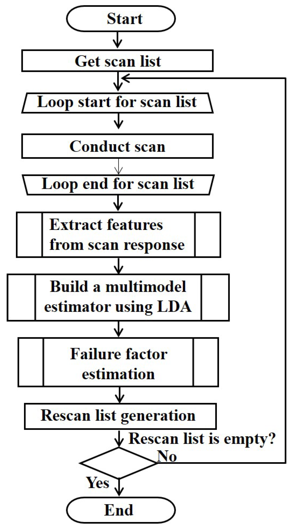
The overall process of the cause estimation algorithm is shown in Figure 1. As shown in Figure 1, the scan list is acquired from the targeted IoT wireless network, and scans are performed on all the ports of the terminals included in the list. Thereafter, the scan response results (such as success, failed, response latency, round-trip time (RTT), etc.) are measured. The scan response features (such as RTT, maximum RTT, jitter, etc.) are extracted and utilized to select the features that are useful for failure factor estimation. Based on the results of the feature selection, we build a multimodel estimator using LDA, as described in Section 4.4. Thereafter, the cause of scan failure/delay is classified into the four causes identified in Section 3—(i) port blocking, (ii) no network connection, (iii) SNR insufficient, and (iv) NW congestion. Terminals that are judged as “SNR insufficient” or “NW congestion” are stored in the rescan list to perform the network scan again, and the process is repeated until the rescan list becomes empty.

4.2. Feature Extraction

Selecting the right feature in any machine learning algorithm is important; however, some features may be more sensitive to the specific cause of failure/delay than others. Using such features in a machine learning algorithm may introduce a bias in the machine learning model. Therefore, in order to avoid this problem, there is a need to determine the importance of the features of the scan response. The scan response RTT is expected to be different in various network scenarios and in each cause of scan failure/delay. For example, in a normal network environment where the communication is not overloaded, the RTT of a scan response is expected to be smaller as compared to when the network is overloaded. It is possible to differentiate the cause of scan failure in these two scenarios. Hence, the scan response RTT is adopted for estimating the failure/delay. However, to achieve the optimal estimation of the cause of scan failure/delay, we find other features that can be combined with the RTT.

To select the best feature that can contribute the most to our cause estimation algorithm, firstly, we performed a series of network scans under various network scenarios. After that, we identified features of the scan response results obtained from the network scans that can be used to distinguish the cause of scan failure/delay. Features such as scan success rate, scan RTT, scan maximum RTT, scan minimum RTT, background traffic packet loss rate, background traffic throughput, etc., may be acquired from a scan response result. However, there are situations in which it is difficult to measure the background traffic; hence, in this paper, we used scan traffic. Secondly, we found the relationship between the scan response RTT and such feature(s) using Pearson correlation coefficient. Thirdly, the significance of each feature was examined and each feature was ranked according to its importance to the factor estimation. Any feature that was ranked as the best feature was extracted and combined with the scan response RTT. The combined data were utilized to build a machine learning model in our estimation algorithm.

4.2.1. Features Significance

To determine the significance of each feature of a scan response, first, we find the correlation between the scan response RTT and other features of the scan response. The correlation coefficient $corr$ for all features in the scan response is calculated as in Equation (1), where N is the number of samples in the scan response, and x and y represent the individual sample points from the scan response RTT and other features, respectively. $\Sigma x$ and $\Sigma y$ are the sample mean of each feature (i.e., the mean sample of the scan response RTT and the mean sample of other features).

$$corr={\displaystyle \frac{N\Sigma xy-(\Sigma x)(\Sigma y)}{\sqrt{[N\Sigma x^2-{(\Sigma x)}^2][N\Sigma y^2-{(\Sigma y)}^2]}}}.$$

(1)

Each feature that is correlated to the scan response RTT is extracted from the scan response. For this, strongly positive or moderately positive correlated features are extracted.

It is possible that a feature may have a high correlation coefficient but contribute less to the factor estimation; therefore, a process to determine the significance of each extracted feature is necessary. In order to determine the significance of each extracted feature when combined with the scan response RTT, statistical multiple linear regression is utilized. In this case, the coefficient of determination (R-squared ($R^2$)) from the linear regression needs to be close to 1. If the $R^2$ is close to 1, the features are considered significant to the factor cause estimation. Otherwise, they are considered as not significant.

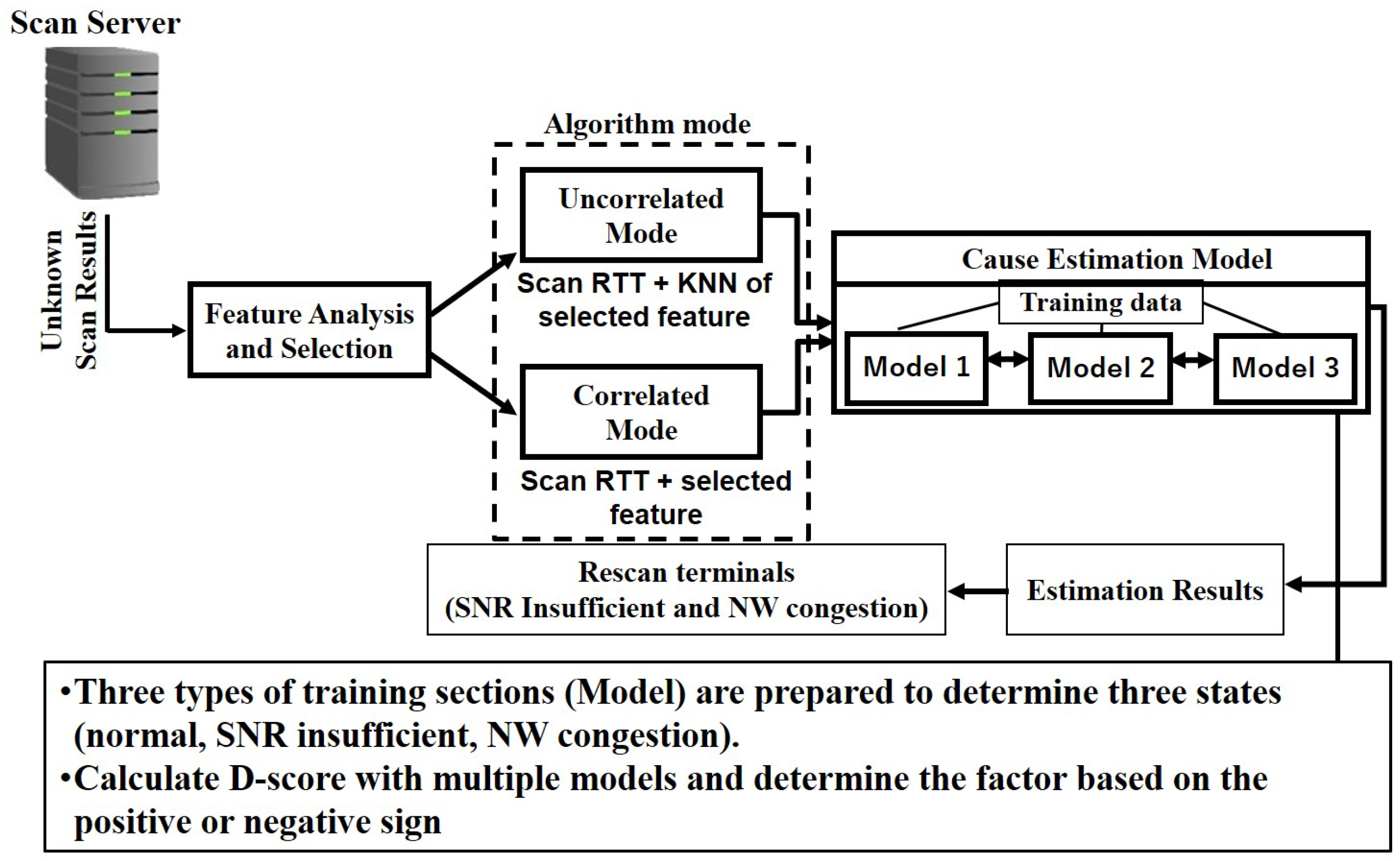
Furthermore, the mode of our factor cause estimation algorithm is divided into two, as shown in Figure 2: uncorrelated mode and correlated mode. In the uncorrelated mode, it is expected that the selected feature has a high/moderate positive correlation coefficient and $R^2$ close to 0 (e.g., $R^2$ = $0.18$). In the correlated mode, however, it is expected that the selected feature has a high positive correlation coefficient and $R^2$ close to 1 (e.g., $R^2$ = $0.8$). Based on these characteristics, the mode of our factor cause estimation is decided. If there are no correlated features, then the uncorrelated mode of the algorithm is used for the failure factor estimation. Additionally, in a situation where the algorithm mode is decided to be an uncorrelated mode, the extracted feature is optimized by calculating the K-nearest neighbor (KNN) [20]. The KNN of the selected feature (i.e., the average value of the distances calculated as in [4]) is combined with the scan response RTT before being passed into the estimation algorithm.

4.2.2. Features Ranking

Another method utilized in our feature selection is the ranking of features. Here, each feature is ranked according to the order of its importance to the factor cause estimation, and the best feature is selected. To determine the importance of features, first, a “chi-square (${\chi }^2$)” statistical test for non-negative feature is used to determine a specified number of features as important. Given a scan response with features $S_1$, $\dots ,$ $S_z$, where z is the total number of features, the scan response features are arranged in a table such that each feature $S_z$ corresponds to the $jth$ column of the table and the values of the data samples $S_{x_m}$ of each corresponding $S_z$ are arranged in the $qth$ row.

Table 2. An example of arrangement of features in a table for feature ranking.

${\mathit{S}}_1$	${\mathit{S}}_2$	${\mathit{S}}_3$	${\mathit{S}}_4$
0	0.022	0.049	0.008
0	0.012	0.034	0.008
0	0.029	0.023	0.008
0	0.009	0.038	0.008
0	0.024	0.022	0.015
0	0.003	0.022	0.015
0	0.004	0.021	0.015
0	0.003	0.023	0.015

shows an example of the arrangement of four scan response features with each $jth$ column of the table corresponding to an unsuccessful scan rate ($s_1$), scan jitter ($s_2$), scan maximum RTT ($s_3$), and scan minimum RTT ($s_4$), respectively. A sample of the scan response data of a feature is denoted as $x_{mq}$, where x represents an individual sample point, m is the index of a sample, and q is the $qth$ row of a sample in the table.

The ${\chi }^2$ is calculated as in Equation (2), where x is the observed value of the data sample of a feature obtained from the scan response results, and m is the index of the value of the feature (i.e., the index of a sample as stated above). E is the expected value of a sample, and it is calculated for each sample value as in Equation (3) by multiplying the sum total $t_q$ of the values of all features in the $qth$ row by the sum total of the values of a feature in the $jth$ column divided by the grand total N. N is calculated as in Equation (4), where $t_q$ is the sum total of the values of all features in a row, and b and n are the index and total number of samples of $t_q$ respectively. Thereafter, the features with the highest $chi$ corresponding to the specified number of features are selected as important features S.

$${\chi }^2=\sum _{m=1}\frac{{(x_m-E)}^2}{E},$$

(2)

$$E=\sum \frac{(t_q\times t_j)}{N}.$$

(3)

$$N=\sum _{b=1}^a{t}_{q_b}.$$

(4)

Furthermore, a recursive feature elimination (RFE) [38] is utilized to select the best feature from the important features described above. The best feature is combined with the scan response RTT to achieve better estimation accuracy. RFE works by recursively removing the feature with the lowest ranking score at each iteration of the algorithm and building a model on those features that remain. It identifies features that can contribute the most to predicting the target class (i.e., the cause of scan response failure/delay).

The process of using RFE is summarized in Algorithm 1 and is performed as follows. From the stored correlated features described above, perform a greedy search to find the best feature by considering smaller and smaller sets of features. Thereafter, train the selected features from S with a classification algorithm (e.g., SVM or LR). Iteratively create models and determine the best or the worst performing feature at each iteration (i.e., find features with the smallest ranking $s_r$). Any feature with the smallest ranking is eliminated. Then, construct the subsequent models with features that are left until all the features are explored. Finally, rank the features based on the order of their elimination and select the top ranked feature $F^1$ as the best feature. For example, using the features stated above (i.e., as in Table 2),

Table 3. An example of features ranking table.

Rank	Features	Weight Score
1	Scan maximum RTT	0.32
2	Scan jitter	0.29
3	Scan minimum RTT	0.25
4	Unsuccessful scan rate	0

shows the ranking table with the weight score (feature ranking score) that is used to eliminate each feature after each iteration. The unsuccessful scan rate is ranked 4 and it is eliminated first, followed by the scan minimum RTT (ranked 3), and then scan jitter (ranked 2) is eliminated after that. The final ranking of the scan response features is completed, with scan maximum RTT having the top rank with a weighted score of $0.32$.

Algorithm 1 Feature ranking.

Require:$S:$ Stored features from scan response Variables: $N:$ Number of correlated features stored Ensure: $F^1:$ Top ranked feature   1: Select the best features from S   2: Train features from S with a classification algorithm (e.g., SVM classifier);   3: Calculate the weight value of each feature;   4: while $N\ne 0$do   5:    Calculate the ranking: ranking of all features in S according to their weight;   6:    Find feature with the smallest ranking: $s_r$ = $argmin\left(ranking\right)$;   7:    Update feature ranked list   8:    Remove feature with the smallest ranking $s_r$ from S    9:    $N\leftarrow N-1$;   10: end while   11: $F^1\leftarrow$ last ranked feature   12: return $F^1$;

4.3. Linear Discriminant Analysis

LDA [39] is a method used to find a linear combination of features that can be used to differentiate two events. The results of such analysis are used in the machine learning classification algorithm. It transforms the features into lower dimension and maximizes the ratio of the between-class variance to the within-class variance; therefore, maximum separation of the classes is guaranteed [22]. LDA spheres the data based on the common covariance and classifies the data to the closest class centroid in the transformed space.

To achieve this, the separability between different classes, which is the distance between the mean of different classes (also known as the between-class covariance), is calculated. Thereafter, the distance between the mean and the samples of each class (also known as within-class covariance) is also computed. From this, the lower-dimensional space which maximizes the between-class covariance and minimizes the within-class covariance is constructed. These properties are unknown beforehand and they are estimated from the training data before being applied to the linear discriminant equation known as discriminant function.

The LDA is given as in Equation (5), where T is the transpose matrix consisting of the rotation of a datum (e.g., vector $\mathit{x}$ and ${\hat{\mathit{\mu }}}_k$). ${\widehat{\mathit{P}}}^{-1}$ is the inverse of the pooled covariance matrix, ${\widehat{\mathit{\mu }}}_k$ is the mean vector of features in the group k, and $log{\widehat{\Pi }}_k$ is the natural log of the prior probability. The pooled covariance matrix is given as in Equation (6), where ${\mathit{x}}_i$ is a sample of scan response result, i is the index of the sample, N is the total number of samples, and K is the total number of group. The prior probability ${\widehat{\Pi }}_k$ is the probability that a sample datum belongs to a group, and is given as in Equation (7), where $N_k$ is the number of samples in a group k.

$${\delta }_k\left(x\right)={\mathit{x}}^T{\widehat{\mathit{P}}}^{-1}{\widehat{\mathit{\mu }}}_k-{\displaystyle \frac{1}{2}}{\widehat{\mathit{\mu }}}_k^T{\widehat{\mathit{P}}}^{-1}{\widehat{\mathit{\mu }}}_k+log{\widehat{\Pi }}_k,$$

(5)

$$\widehat{\mathit{P}}={\displaystyle \frac{{\Sigma }_{k=1}^K{\Sigma }_{g_i=k}({\mathit{x}}_i-{\widehat{\mathit{\mu }}}_k){({\mathit{x}}_i-{\widehat{\mathit{\mu }}}_k)}^T}{(N-1)}},$$

(6)

$${\widehat{\Pi }}_k=(N_k/N),$$

(7)

$${\widehat{\mathit{\mu }}}_k={\Sigma }_{g_i=k}{\mathit{x}}_i/N_K.$$

(8)

Using the discriminant function as stated above, for an unknown data sample x, the discriminant score $D_s$ can be calculated for each class, as explained later. The data sample x is classified into the class having the highest score.

To create a model using the standard LDA, first, the training data are separated into different groups based on the number of scenarios we want to estimate. To separate the training data into different groups, the data samples are divided into equal sizes corresponding to the number of scenarios we wanted to estimate (i.e., 3—normal, low SNR, and congestion). Thereafter, the mean of each group is calculated. Then, the global mean of the whole data and the prior probability of each group are calculated. If the total number of samples of each scenario to be estimated is not known, then the prior probability is estimated by assuming that the total number of samples of each scenario is equal. The next step is to calculate the pooled covariance, as described above. Lastly, the pooled covariance is used to generate the inverse of the pooled covariance. Each variable is then applied to the discriminant function as in Equation (5).

However, the network environment dynamically changes and it is not possible to know the distribution of the scan response beforehand. Generally, the standard LDA requires that the distribution of the data sample must be Gaussian in order for the classifier to preserve the complex structure that is needed to reduce the classification error. In addition, the standard LDA will fail when the information that is needed to discriminate samples is not found in the mean value of the sample. Therefore, a method that can reduce the classification error is required.

4.4. Multimodel Estimator

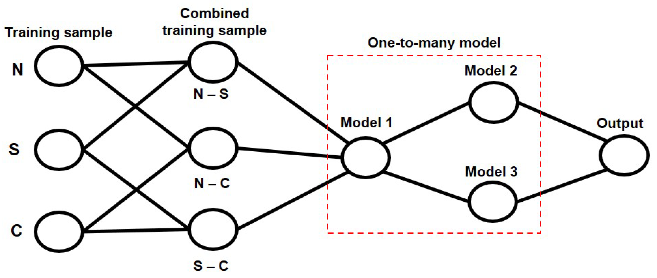
To estimate the cause of scan failure/delay where the conventional machine learning classifiers fail to correctly estimate new samples (i.e., cannot generalize samples of new scan response results), we propose an MM-LDA. Specifically, a two-class LDA is used to build a one-to-many model in our cause estimation algorithm, where three types of training data obtained from different network scenarios (i.e., normal, low-SNR, and congestion) are extracted as described above and combined to build each model. Figure 3 shows the cause estimation process used for the proposed MM-LDA, where the training samples N, S, and C correspond to the scan response results obtained from various scenarios (i.e., N—normal, S—low SNR, and C—congestion). To create the cause estimation model which is used in our estimation algorithm, firstly, as described in Section 4.2, we identify and select from the scan response the best features that can be used to estimate the cause of scan failure/delay and are combined with scan response RTT. Then, the combined data are used to create a training data set for our model. For this, three types of training sections (models) are prepared to determine the causes of scan failure/delay (i.e., normal, SNR insufficient, and NW congestion).

As shown in Figure 3, each separated group of our training data is combined to create a model. The network scan traffic data from various scenarios are combined in the following order: model 1—normal and low SNR, model 2—normal and congestion, and model 3—low SNR and congestion. Thereafter, using a one-to-many model, the combined training samples are passed into the model. Based on the result obtained, the next model to be utilized is determined (e.g., if the scan response is determined to be normal in the first model, then the second model is selected as the next model; otherwise, the third model is selected). This approach will help to reduce the estimation error of the scan failure/delay where the data samples obtained in various scenarios overlapped.

In our MM-LDA, two discriminant functions, $f^1$ and $f^2$, are calculated for each model. The data samples from the combined training data that correspond to each separate group are used to calculate the covariance matrix ${\mathit{C}}_k$ as in Equation (9), where ${\mathit{x}}_k$ are the data samples of a group k, and $N_K$ is the number of samples in the group k. Thereafter, the pooled covariance matrix ${\widehat{\mathit{C}}}_{uv}$ is calculated for each model as in Equation (10), where ${\mathit{C}}_k$ is the data value of the covariance matrix $\mathit{C}$ of a group k in the combined training data, and N is the number of samples of the combined training data. u and v correspond to the group k of the combined training data in each model such that when the training sample from the normal and low SNR scenarios are combined, u = 1 and v = 2. L denotes the number of groups in the combined training sample. Each value of the pooled covariance is calculated separately using the corresponding values of the covariance matrix of the combined training data for each model. Furthermore, the inverse of pooled covariance ${\widehat{\mathit{C}}}_{uv}^{-1}$ is calculated and applied into the discriminant function of each model (e.g., Equation (11)).

$${\mathit{C}}_k={\displaystyle \frac{{\mathit{x}}_k{\mathit{x}}_k^T}{N}},$$

(9)

$${\widehat{\mathit{C}}}_{uv}=\sum _{k=1}^L{\displaystyle \frac{{\mathit{C}}_k{N}_k}{N}}.$$

(10)

In addition, as given in Equations (11)–(16), the mean $\mu$ and the prior probability $log\Pi$ are calculated based on the size of the training data for each separate group (i.e., $k_1$—normal, $k_2$—low SNR, and $k_3$—congestion) of training data in each model.

Model 1:

$$f^1={\mathit{x}}^T{\widehat{\mathit{C}}}_{12}^{-1}{\widehat{\mathit{\mu }}}_{k_1}-{\displaystyle \frac{1}{2}}{\widehat{\mathit{\mu }}}_{k_1}^T{\widehat{\mathit{C}}}_{12}^{-1}{\widehat{\mathit{\mu }}}_{k_1}+log{\widehat{\Pi }}_{k_1},$$

(11)

$$f^2={\mathit{x}}^T{\widehat{\mathit{C}}}_{12}^{-1}{\widehat{\mathit{\mu }}}_{k_2}-{\displaystyle \frac{1}{2}}{\widehat{\mathit{\mu }}}_{k_2}^T{\widehat{\mathit{C}}}_{12}^{-1}{\widehat{\mathit{\mu }}}_{k_2}+log{\widehat{\Pi }}_{k_2}.$$

(12)

Model 2:

$$f^1={\mathit{x}}^T{\widehat{\mathit{C}}}_{13}^{-1}{\widehat{\mathit{\mu }}}_{k_1}-{\displaystyle \frac{1}{2}}{\widehat{\mathit{\mu }}}_{k_1}^T{\widehat{\mathit{C}}}_{13}^{-1}{\widehat{\mathit{\mu }}}_{k_1}+log{\widehat{\Pi }}_{k_1},$$

(13)

$$f^2={\mathit{x}}^T{\widehat{\mathit{C}}}_{13}^{-1}{\widehat{\mathit{\mu }}}_{k_3}-{\displaystyle \frac{1}{2}}{\widehat{\mathit{\mu }}}_{k_3}^T{\widehat{\mathit{C}}}_{13}^{-1}{\widehat{\mathit{\mu }}}_{k_3}+log{\widehat{\Pi }}_{k_3}.$$

(14)

Model 3:

$$f^1={\mathit{x}}^T{\widehat{\mathit{C}}}_{23}^{-1}{\widehat{\mathit{\mu }}}_{k_2}-{\displaystyle \frac{1}{2}}{\widehat{\mathit{\mu }}}_{k_2}^T{\widehat{\mathit{C}}}_{23}^{-1}{\widehat{\mathit{\mu }}}_{k_2}+log{\widehat{\Pi }}_{k_2},$$

(15)

$$f^2={\mathit{x}}^T{\widehat{\mathit{C}}}_{23}^{-1}{\widehat{\mathit{\mu }}}_{k_3}-{\displaystyle \frac{1}{2}}{\widehat{\mathit{\mu }}}_{k_3}^T{\widehat{\mathit{C}}}_{23}^{-1}{\widehat{\mathit{\mu }}}_{k_3}+log{\widehat{\Pi }}_{k_3}.$$

(16)

In our model, the $D_s$ of each terminal is calculated as given in Equation (17) using the selected model.

$$D_s=f^1-f^2.$$

(17)

Finally, in order to optimize the performance of our MM-LDA and reduce bias estimation, which may occur when some features are more sensitive to a particular cause of scan failure/delay than the others or when the causes of scan failure are highly imbalanced in the training dataset (i.e., each cause is not equally represented in the training data), we adopt a method to filter the training set used in creating the MM-LDA model based on the variance of the scan response RTT. Here, we find the variance of the scan response RTT of each separated group of scan response obtained in the three scenarios (normal, low SNR, and congestion). The scan response RTT samples with a variance higher than their group are removed from the training set used in creating the MM-LDA model of that group.

5. Cause of Scan Failure/Delay Estimation

In order to estimate the cause of scan response failure/delay, our proposed MM-LDA calculates the discriminant score ($D_s$) for each terminal connected to a base station, access point, etc., and based on the result of the calculated $D_s$, the normal scan situation is determined if the $D_s$ is positive or equal to 0 (i.e., $D_s\ge 0$), and the abnormal scan situation is determined if $D_s<0$.

To judge each failure factor for all terminals connected to a base station, access points, etc., the number of terminals $D_{count}$ with an abnormal value (i.e., $D_s<0$) are counted. If 0 < $D_{count}$ < ($N_{terminals}\ast D_{thres}$), then the failure factor of the terminals with the abnormal value is judged as SNR insufficient. $N_{terminals}$ is the total number of terminals connected to a base station/access point, while $D_{thres}$ ($D_{thres}$ is a real number with the range of 0–1) is the cutoff threshold between insufficient communication quality and network congestion. On the other hand, if $D_{count}$ ≥ ($N_{terminals}\ast D_{thres}$), the failure factor for all terminals connected is judged as NW congestion. All terminals are judged as normal when $D_{count}$ = 0.

Thereafter, the next step is to determine whether there is a scan response result for each terminal that does not fall under either SNR insufficient or NW congestion. In such a situation, if there is no response at all ports of the terminal, it is determined as no network connection for the terminals, while for terminals that have a response from any port, the ports with no response are judged as port blocking. The complete estimation process is summarized as follows.

• Extract the scan response RTT and other features from the scan response results of each scenario.
• Calculate the correlation of several features in each scenario.
• Similarly, calculate the multiple linear regression and determine if the features are significant and should be selected as correlated features or uncorrelated features.
• Apply the RFE algorithm on the selected features and ranked features based on their importance to the factor cause estimation, as in Algorithm 1.
• Combine the scan response RTT data and the top ranked feature.
• Normalize missing data by replacing them with a constant negative value in the range of [−999, −1], etc. This is to prevent bias influence on the cause estimation result.
• Create a training dataset, which is used to build estimation models using MM-LDA. Divide the training data into three datasets and build three models.
• For each terminal connected to a base station, access points, etc., using a one-to-many model, pass the scan response RTT samples into the first model, and the discriminant score $D_s$ is calculated. If the $D_s$ is positive or equal to 0 (i.e., $D_s\ge 0$), a normal scan situation is determined, and the second model is selected. Otherwise (i.e., $D_s<0$), an abnormal scan situation is determined, and the third model is selected. Calculate $D_s$ for each terminal and judge the cause of scan failure/delay based on the result of the selected model.
• Count the number of terminal ($D_{count}$) with $D_s$ < 0. If 0 < $D_{count}$ < ($N_{terminals}\ast D_{thres}$), then the terminal with the abnormal value is estimated as SNR insufficient. If $D_{count}$ ≥ ($N_{terminals}\ast D_{thres}$), then all terminals are estimated as NW congestion. All terminals are estimated as normal when $D_{count}$ = 0.
• For each terminal that is not estimated as SNR insufficient communication quality or NW congestion, check if there is no response from all ports. If there is no response at all ports of the terminal, the cause for the terminal is estimated as no network connection. Otherwise, the terminal is judged as normal, and the cause for the ports of the terminal with no response are estimated as port blocking.

6. Evaluation

We evaluate the estimation accuracy of the failure factor estimation algorithm. The performance evaluation is conducted using the scan response results acquired through a computer simulation using ns-3 (version 3.30) [40]. The scanning mechanism used in our simulator is similar to that of state-of-the-art scanning tools, such as Masscan, which is capable of transmitting up to 10 million packets per second. The scan response data in the “normal”, “low SNR” (a scenario in which the propagation loss of a certain terminal is large), and “congestion” scenarios are acquired assuming a cellular system (LTE). This simulation does not consider “port blocking” and “no network connection”. A port that is blocked by a firewall is considered safe and is reported as “filtered” or “blocked”, while the result of the network scan when there is “no network connection” will result in a time-out, and no actual data can be gathered when these causes of scan failure/delay occur.

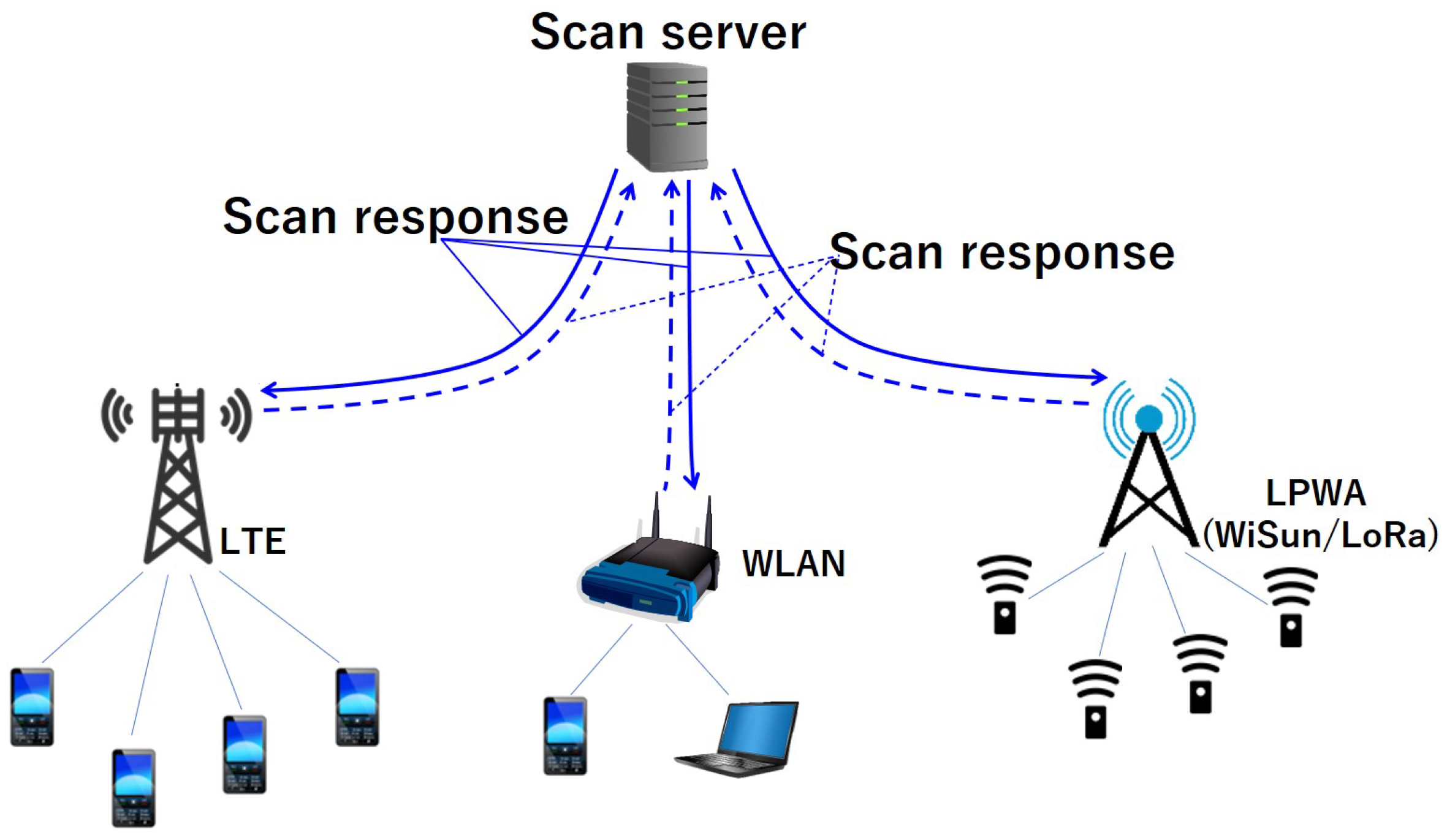
Figure 4 shows the target network in our study. In this evaluation, only the LTE network is considered. In the future, we will expand the cause estimation to the low-power wide-area (LPWA) (Wi-SUN/LoRa) networks.

6.1. Simulation Configurations

The simulation is implemented by performing a network scan for each scenario in various samples. In our simulation, the terminals are randomly placed around the base station. We acquired 1000 patterns each for two sets of scan response samples of each scenario.

Table 4. Simulation settings.

Parameter	Value
	Set 1	Set 2
Simulation time	300 s	300 s
Number of base stations	1
Number of terminals	8 (4 each for UL/DL background traffic)
Terminal arrangement range	20 m square, 250 m square around the base station	20 m square, 200 m square around the base station
Propagation model	ITU base coverage urban, urban macro-cell scenario [41]
Scheduling method	Proportional fairness
System bandwidth	5 MHz
Background traffic
Applied traffic volume	1, 8 Mb/s (per terminal)
Occurrence size	1250, 10,000 bytes
Occurrence interval	10 ms
Packet size	1000 bytes
Protocol	UDP
Occurrence start time	1 s
Scan traffic
Open port	1–100	1–1000
Scanned port	1–100	1–1000
Timeout period	100 ms
Applicable time	2 s
Packet size	60 bytes
Failure factor estimation
Number of model	3
$D_{thres}$	0.5

shows the simulation settings and the parameters. The number of terminals for each pattern in the two sets is 8, and the number of ports scanned are 100 and 1000, respectively.

Our simulator is capable of performing a network scan on all 65,536 ports in both UDP and TCP. On a real device, it is not all ports that are commonly used, and most ports are completely disabled or blocked by the firewall. Therefore, the complete 65,536 ports are not needed to show the performance of our method. Additionally, the performance of the proposed estimation method is not limited to the number of ports scanned. Furthermore, in this simulation, ports based on the TCP protocol are not considered. A total of 24,000 data samples (i.e., 8 terminals per pattern × 1000 patterns × 3 scenarios) were acquired for each of the first and second simulation sets.

Furthermore, settings such as terminal arrangement range and background traffic volume were set to be different between scenarios and samples generated from the scan response data in different situations. The following differences were made for each scenario: set 1—(i) “normal”—20 m, 1 Mb/s; (ii) “low SNR”—250 m, 1 Mb/s; and (iii) “congestion”—250 m, 8 Mb/s. Set 2— (i) “normal”—20 m, 1 Mb/s; (ii) “low SNR”—200m, 1 Mb/s; and (iii) “congestion”—200 m, 8 Mb/s. In the “low SNR” scenario, only a specific terminal is fixed at a distance from the eNB, so that the communication quality of a certain terminal deteriorates due to large propagation loss. Furthermore, the simulation setting is configured such that the signal-to-noise ratio for the low SNR is in the range between 3–10.5 dB.

6.2. Results and Discussion

6.2.1. Data Analysis

In order to estimate the cause of network scan failure/delay, it is necessary to examine the distribution of multiple QoS features of the scan response. The distribution is expected to be different in various scenarios. In addition, the distribution of features is expected to be different in relation to the network scan response RTT in two distinct scenarios. Therefore, the first step is to examine the attributes of the scan responses acquired in various network states.

As explained in the previous section, the scan response was obtained by performing a network scanning in various scenarios (e.g., normal, low SNR, and NW congestion). Each scenario was equally distributed with 33.3% distribution ratio in the simulation.

6.2.2. Scan Response Rate

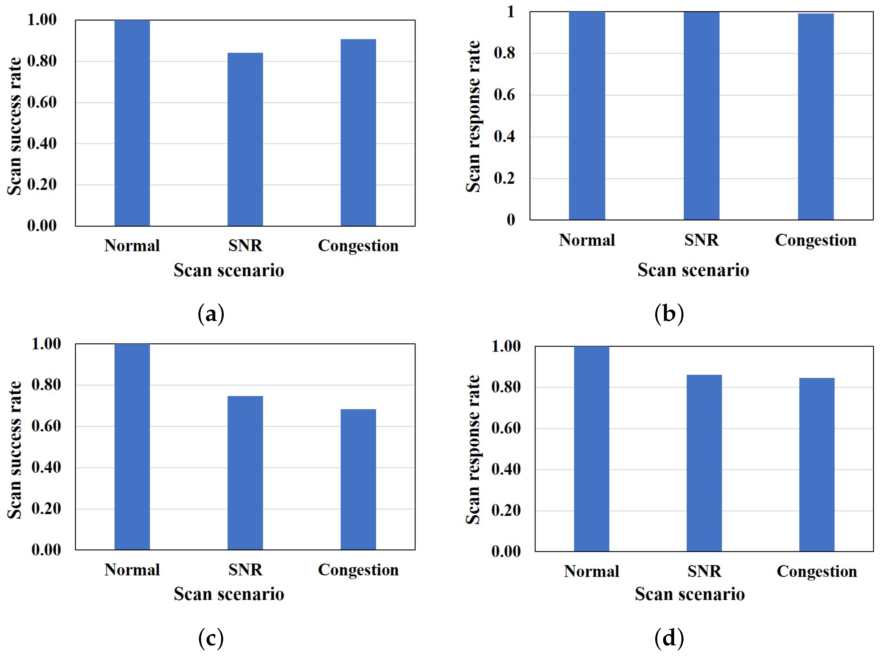
To evaluate the performance of the cause estimation algorithm, firstly, we analyze the results of the network scan response acquired. Figure 5 shows the success rate of the network scan in three scenarios in our simulation. The scan response rate is the rate at which the network scanner can acquire a response (i.e., an ACK packet is received) from the terminal, irrespective of a successful scan or not, without dropping the response packet (i.e., number of ACK response received/number scan packet sent). The scan success rate is the rate at which the executed scan on a terminal port is successful (i.e., number of successful scanned ports per terminal/number of ports scanned per terminal). From the simulation results, as shown in Figure 5a,c, in the first set, an average of almost all scan packets were successful in the normal scenario. A success rate of an average of 84% and 91% was observed in the low SNR and congestion scenarios, with an average of 16% and 9% network scan failure rates. On the other hand, in the second set of the scan response sample, we observed that all the scan packets were successfully delivered in the normal scenario with a success rate of 100%, while the success rates in low SNR and congestion scenarios are 75% and 68% on average. Averages of 25% and 32% network scan failure rates were observed in the low SNR and congestion scenarios, respectively, for the second set of the scan response sample. This confirms the settings of our scenarios, from which the estimation of the cause of scan failure can be realized. Figure 5b,d show that there is a high response rate of terminals to the network scan with over 80% response rate in all scenarios in both sets of scan response samples, and a scan packet loss rate of 15% and 16% in the second set.

6.2.3. Scan Response Distribution

According to the analysis of the scan response data and their features, we observed that there are situations in which the scan response samples from a particular scenario are linearly separable from the scan response samples of the other scenarios. On the other hand, the scan response samples of the other scenarios are not linearly separable from each other. This can make it difficult to apply conventional machine learning to classify these scan response data.

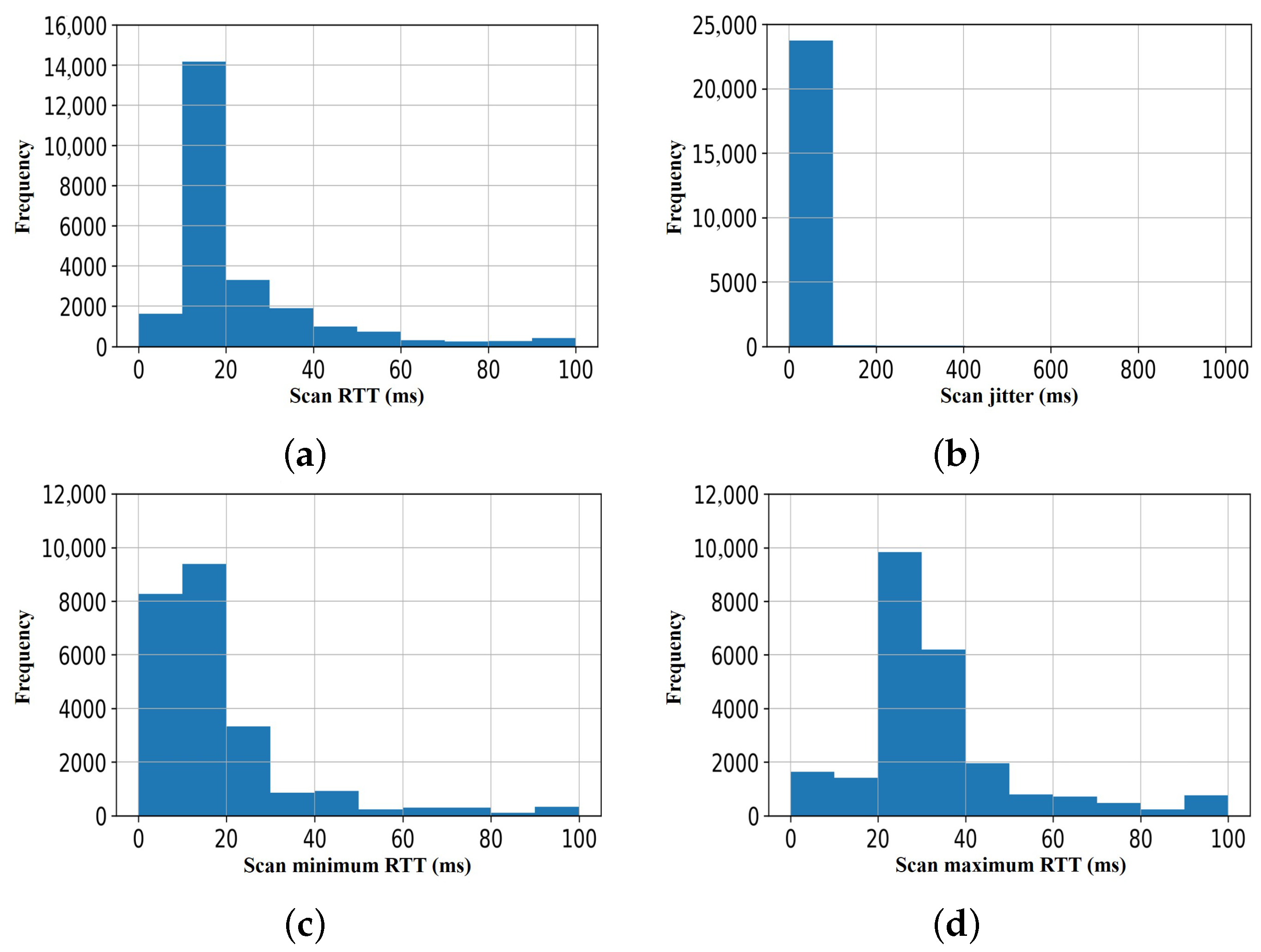
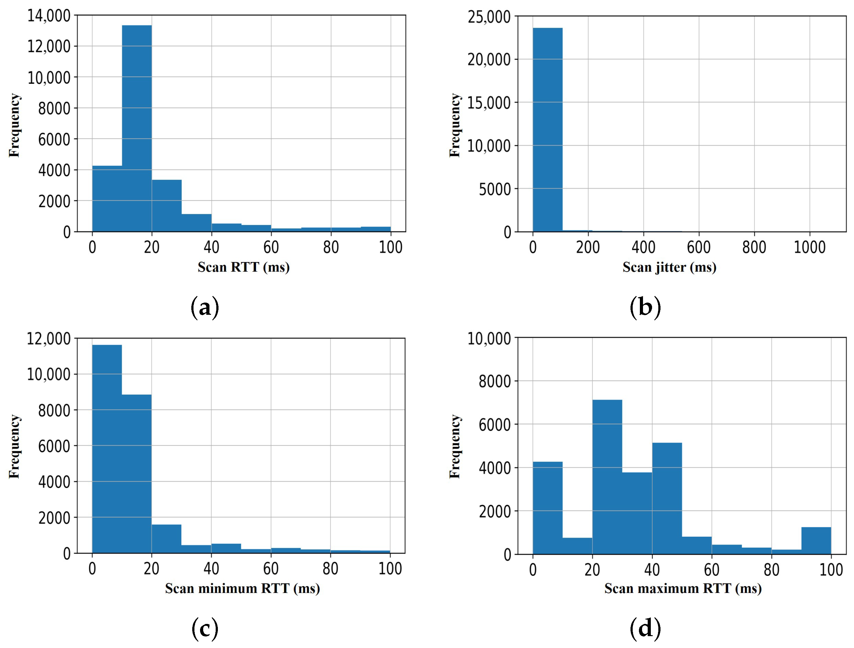
As shown in Figure 6a–c, we observed that the distribution of features (scan traffic data) of the scan response data obtained in the first sample set is non-Gaussian distribution, although the maximum RTT (shown in Figure 6d) may be described as approximately Gaussian. Similarly, as shown in Figure 7, for the second set of the scan response samples, we observed that three out of the scan traffic features are non-Gaussian distributed.

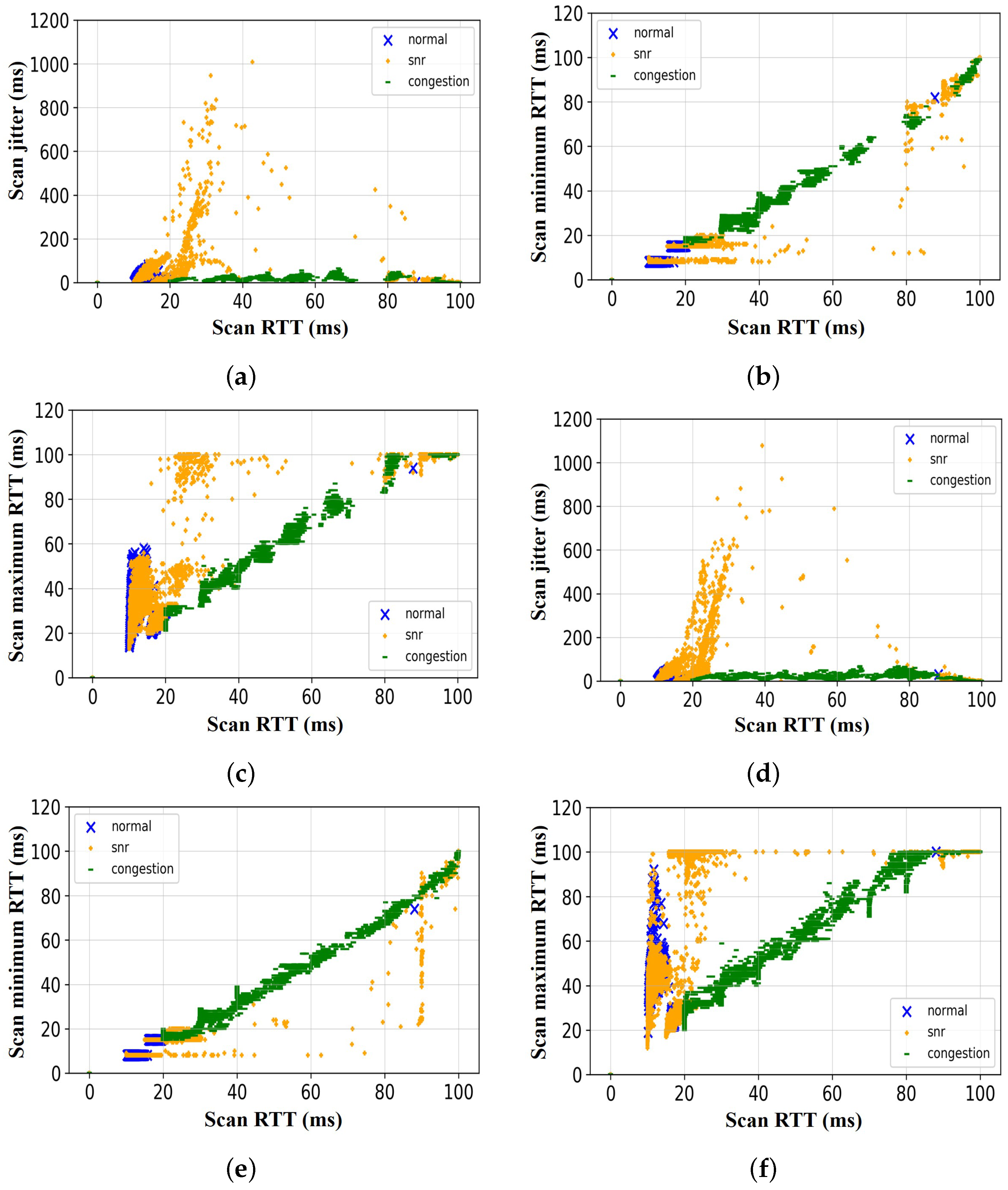
Furthermore, Figure 8 shows the details of the relationship between the features of the scan response samples of each scenario—normal, low SNR, and congestion (i.e., which scan response feature can be used in combination with the scan response RTT to classify the cause of scan failure/delay). As shown in Figure 8a, for the first sample set, we observed that when using scan response RTT and scan response jitter, we can only distinguish the scan response data obtained in the congestion scenario from the other two scenarios (i.e., normal and low SNR scenarios). We confirmed that the scan response acquired in the normal scenario and the low SNR scenario mostly overlap. The same trend was observed when the other two features (i.e., minimum RTT and maximum RTT) were analyzed in relation to the scan response RTT. Figure 8b,c show that it is only possible to distinguish the scan response data obtained in the congestion scenario from the other two scenarios.

In the second sample set, however, as shown in Figure 8d, we observed that when using scan response RTT and scan response jitter, we can only distinguish the scan response data obtained in the congestion scenario from the scan response data obtained in the low SNR scenarios. We confirmed that the scan response samples acquired in the normal scenario mostly overlap with the scan response samples of the other scenarios (i.e., low SNR and congestion scenarios). Similarly, as shown in Figure 8e, we observed that only the scan response samples of two scenarios can be distinguished (i.e., low SNR and congestion scenarios) when the scan response RTT and the minimum scan response RTT samples of all the scenarios were examined. The same trend is observed when the maximum scan response RTT feature is analyzed in relation to the scan response RTT. Figure 8f shows that it is only possible to distinguish the scan response data obtained in the congestion scenario from the other two scenarios. In addition, the relation between the scan response RTT and other features of the scan response samples obtained in various scenarios show that only scan response samples of a particular scenario can be linearly separated from the scan response samples of other scenarios. The features of the scan response samples are completely overlapped in two scenarios, as shown in Figure 8. Therefore, a method to achieve a good separation measure is required.

6.2.4. Feature Selection for MM-LDA Model

In order to select the most significant feature that can achieve the optimal estimation of the cause of scan failure/delay, first, we find the correlation between the scan response RTT and other scan response features. As shown in

Table 5. Correlation coefficients of scan response of the training data.

	Scan RTT	Scan Jitter	Scan Maximum RTT	Scan Minimum RTT
Scan RTT	1	0.054	0.869	0.988
Scan jitter	0.054	1	0.371	−0.040
Scan maximum RTT	0.869	0.371	1	0.817
Scan minimum	0.988	−0.040	0.817	1

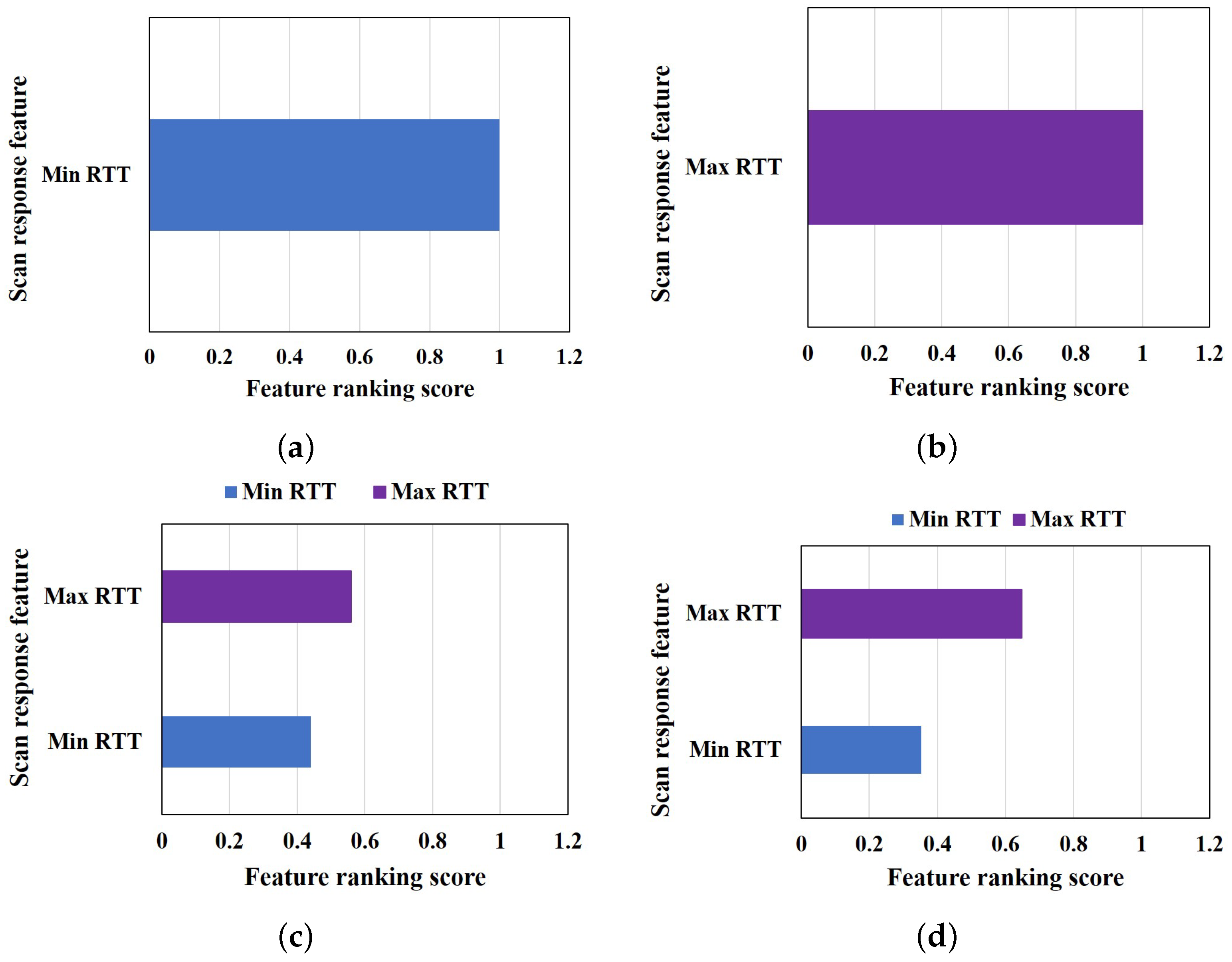
, we observed that the scan minimum RTT and scan maximum RTT were correlated to the scan response RTT with an average of 0.87 and 0.99 correlation coefficients, respectively. Furthermore, we apply the feature selection method to the correlated features. Figure 9 shows the results of feature selection of each scenario. The number of features ranked, as shown in Figure 9, vary based on the correlated feature in each scenario. Only one feature is correlated with the scan response RTT in the normal and low SNR scenarios, while two features are correlated with the scan response RTT in the congestion scenario and when the training data are used for the feature selection. The correlated feature is used for the feature selection. The minimum RTT is selected for a normal scenario with a 1.0 feature ranking score, as shown in Figure 9a. On the other hand, maximum RTT is selected as the best feature for the low SNR scenario, with 1.0 feature ranking score, and for the congestion scenario, with 0.56 ranking score, as shown in Figure 9b,c, respectively. Since there is no common feature among all scenarios and as explained above, only one feature can be linearly separable from other features; therefore, the training data are used to select the best feature, and the uncorrelated mode of the estimation algorithm is used for failure factor estimation.

Moreover, using the training data will prevent bias selection, as different features may be more sensitive to a particular cause of scan failure/delay than the others if features are selected based on each scenario without a common feature among the scenarios. We apply the feature selection method to the correlated features of the training data shown in Table 5. Figure 9d shows the result of the feature that is selected as useful for cause estimation when the training data are utilized. Here, the maximum RTT is selected as the best feature that is useful for the estimation algorithm, with a ranking score of 0.65 feature ranking scores.

6.2.5. Training and Testing Samples

In general, it is widely known that using a small size of training dataset will cause a machine learning model to perform poorly due to underfitting of the training dataset. On the other hand, if the training dataset is too large, it will cause overfitting of the training data. Similarly, too few test data may result in a high variance estimation of the model performance [42]. Therefore, to ensure that the cause estimation algorithm can be generalized when applied to a newly acquired scan response sample, we filter the training samples that are used in building the MM-LDA model by removing scan response samples with high RTT variance in each scenario. For this, the training sample is divided into multiple slices. To pick training sets that can be used for building a new model, each training datum in the slice is selected by a random selection and is used to build a model. Any training datum of a model that failed to outperform the initial model performance threshold (e.g., achieving a 95% correct estimation) is dropped from the training set used in building the model. Thereafter, the training and test samples were selected from the first set of simulation samples for each scan response scenario using a conventional split of 80%/20% for training/test split, respectively. The selected training samples from the filtered training data of each scan response scenario are used to train the model, and the test set, which is not used to train the model, is used to estimate how well the model will generalize when applied to newly acquired scan response data.

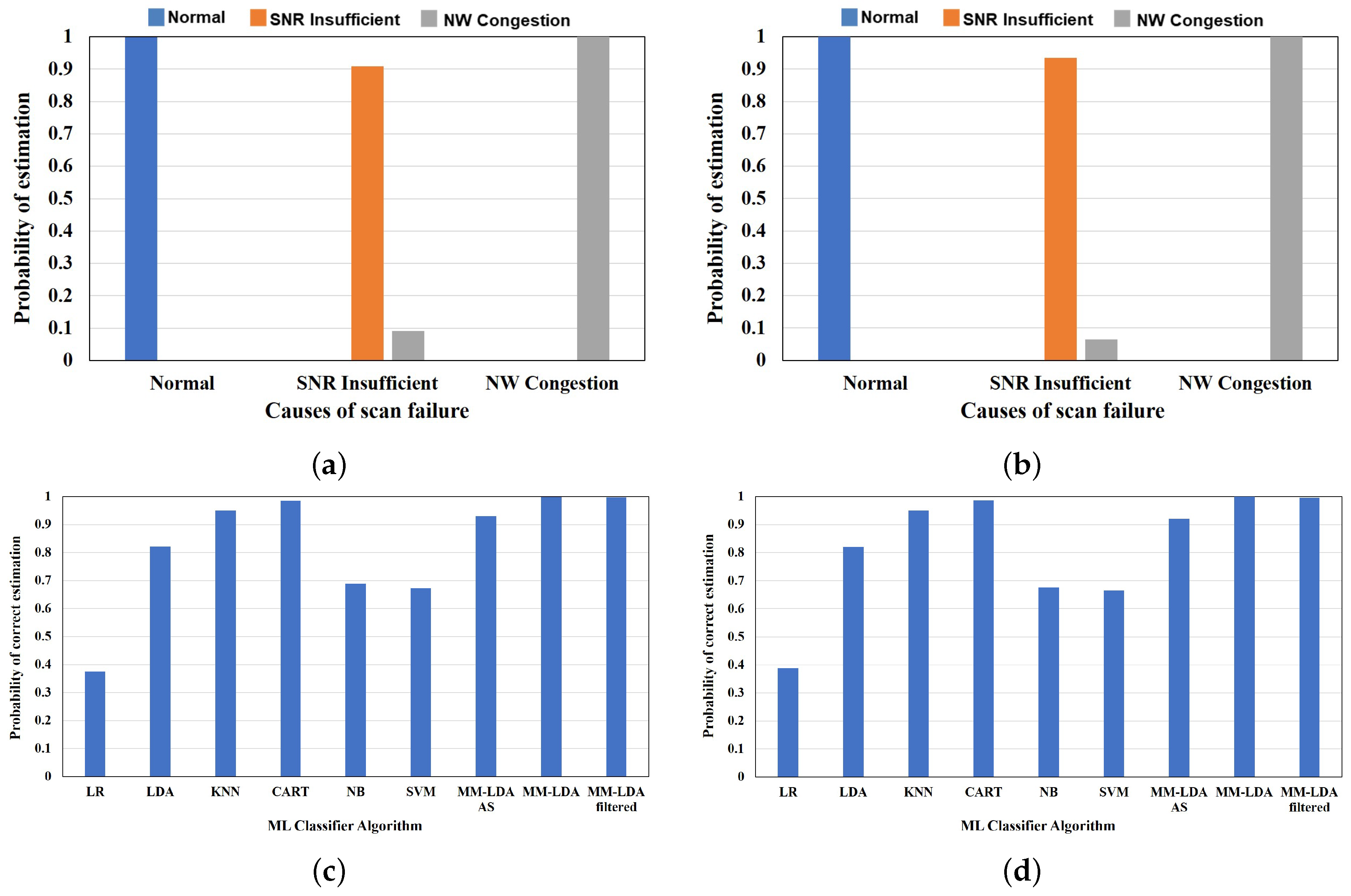
Figure 10 shows the correct estimation ratio of the scan failure/delay of training and test data samples. The first set of results shows the correct estimation ratio of the proposed MM-LDA filtered for the training and test data, respectively. In the second set of results, we compare the performance of the proposed MM-LDA filtered on the training and test data with the performance of other conventional machine learning classifiers. As shown in Figure 10a, the proposed MM-LDA with filtered training set achieves an average of 98% correct estimation of the cause of scan failure/delay (i.e., normal—1.0, SNR insufficient—0.91, and NW congestion—1.0 correct estimation ratio).

Similarly, an average of 97% correct estimation (i.e., normal—1.0, SNR insufficient—0.94, and NW congestion—1.0 correct estimation ratio) is confirmed for the test set, as shown in Figure 10b. In comparison to other conventional machine learning algorithms, as shown in Figure 10c,d, we confirm that LR, NB, and SVM classifiers perform poorly in the estimation of both the training and test data, with estimation results below 70%. On the other hand, KNN and CART achieve high estimation of both the training and test data with 95% and 98% estimation results, respectively. However, only the MM-LDA with the filtered training set is able to generalize new scan response where all the conventional methods fail (see Section 6.2.6).

6.2.6. Cause Estimation of Scan Response of New Scan Response

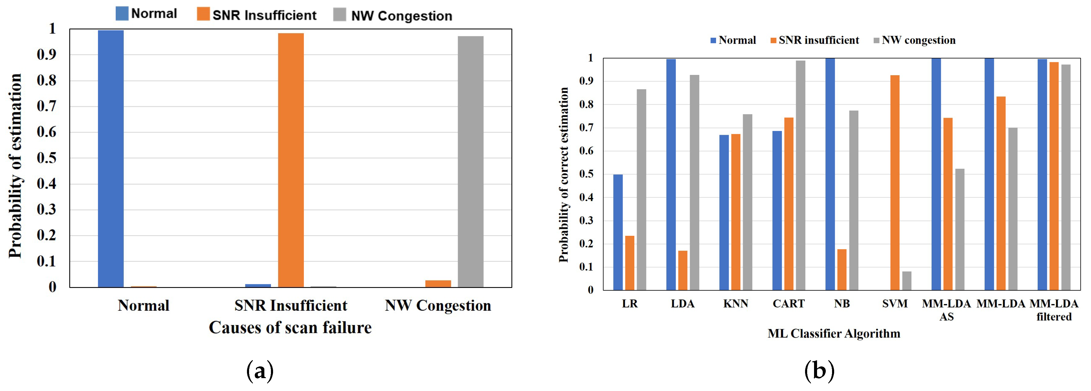
Based on the trained MM-LDA model, we validate the performance of the MM-LDA model by evaluating the proposed multimodel cause estimation algorithm using various scenarios of the second set of simulation samples. According to the results, it is possible to estimate the cause of scan failure/delay correctly using the MM-LDA. Figure 11a shows the results of the estimation algorithm evaluation assuming a cellular system (LTE). From these results, we confirm that the cause of scan failure/delay can be estimated with an average of 98% correct estimation (i.e., normal—1.0, SNR insufficient—0.98, and NW congestion—0.97 correct estimation ratio) of the cause of scan failure/delay in various scenarios when the proposed method is utilized.

6.2.7. Comparison of the MM-LDA to Conventional Methods

The proposed method is compared to other conventional methods stated in Section 2 to show the effectiveness of the proposed method. Figure 11b shows the comparison results when the proposed method is used compared to various conventional machine learning classifiers. The cause of scan failure/delay of various scenarios in the second set of scan response samples obtained through simulation is estimated using the trained model explained in Section 6.2.5. According to the results, we confirm that the proposed MM-LDA with filtered training set outperforms other conventional machine learning classifiers with an average of 98% correct estimation of various causes of scan failure/delay. Although the conventional LDA is able to estimate normal scan response situation and failure/delay caused by NW congestion correctly with 90% correct estimation, it fails to estimate failure/delay caused by SNR insufficient, with only 17% of the sample estimated correctly. Similarly, the CART classifier, which is able to estimate the cause of scan failure/delay correctly in both training and test samples, fails to generalize the new scan response sample. Only the failure/delay caused by NW congestion is correctly estimated, with 99% estimation. In addition, NB and SVM are able to estimate normal scan response and failure/delay caused by SNR insufficient correctly, with 100% and 93% estimation, respectively. This confirms that the proposed MM-LDA with filtered training set does not overfit or underfit the training set.

7. Conclusions

It is essential to know the causes of network scan failure/delay in relation to the communication environment status in order to apply necessary countermeasures against cyberattacks. This paper proposed a method to improve the network scan failure/delay cause estimation using a multimodel-based approach. The causes of network scan failure/delay were identified and analyzed in relation to the communication environment status and communication results in wireless communication systems/networks.

Specifically, a pre-evaluation process of cause of network scan failure estimation was adopted, and a feature that is useful for estimating the cause of scan failure/delay was identified from the scan response features, such as minimum RTT, maximum RTT, jitter, etc. In addition, an MM-LDA was proposed to build a one-to-many model for our proposed method. Using the MM-LDA, a discriminant score $D_s$ was calculated for each terminal connected to a base station, access points, etc., and based on the number of terminals with negative $D_s$, cause of scan failure/delay was judged as SNR insufficient or NW congestion. Furthermore, a filtering process was adopted to improve the performance of the proposed MM-LDA and to reduce bias estimation, which may occur when some features of the scan response data obtained in various scenarios are more sensitive to a particular cause of scan failure/delay than the others.

The performance evaluation of our proposed method was conducted using the scan response results acquired through a computer simulation. The proposed MM-LDA with filtered training data achieved high performance when utilized to estimate the cause of scan failure/delay. The result shows that the proposed method achieved a high estimation result of the cause of scan failure/delay with an average of 98% correct estimation (i.e., normal—1.0, SNR insufficient—0.98, and NW congestion—0.97 correct estimation ratio) of the cause of scan failure/delay in various scenarios. The MM-LDA outperformed various conventional machine learning classification methods.

In the future, we will consider extending the proposed method to other networks, such as Wi-Fi, Wi-SUN, LoRa, etc., by performing a network scan on the IoT wireless devices that are connected to the network and conducting evaluations that assume more realistic situations. In addition, the analysis of the computational and storage complexity of the proposed method compared to the conventional approaches will be examined. Moreover, we will conduct experiments to evaluate our proposed method and consider an estimation based on a deep learning method.