A 2D Quasi-Static Nonlinear Tire Model with Numerical Approximations

Abstract

Tires are the interface between a vehicle and the ground, through which forces and moments are generated. They are therefore critical components of a vehicle, creating a need to estimate their performance under various conditions. The tire model proposed in this study models the tire as an elastic beam on an elastic foundation, similar to a flexible ring model but with more nonlinear terms justified and included. It offers quick and accurate estimates for spindle force and longitudinal pressure distribution with little computational effort. The model is analytically derived with the energy method, building strong connections among the model parameters and physical properties of the tire. It is then solved with numerical approximations. The simulation results show good alignment with the experimental data.

1. Introduction

The fundamental excitation to the vehicle is at the tire–road interface through which the forces and moments of the vehicle are generated and reacted. It is therefore important to model the tire under various loading conditions. The finite element analysis is widely adopted to offer comprehensive results including spindle force, friction, traction, etc. The concern is that a finite element model generally requires considerable effort to calibrate and to calculate. There are situations where using a FEM is redundant; for example, the detailed stress distribution in the tire materials is not as useful for a vehicle handling study. During the initial stage of a tire design process with a preliminary prototype, using a FEM may prolong the time required for each design iteration. Such situations create a need for quick estimates for tire performance. Empirical models are useful tools to meet this need. However, an empirical model is practically a deliberately fitted curve, making it hard to connect the model parameters to the tire properties. Hence, there is a need for analytical or semi-empirical models, of which the equations are derived from the tire physics and mechanics to create strong correlations among the model parameters, tire performance and tire properties. Since a large part of calculations are pre-completed during the derivation and construction of the model, the computational effort is greatly reduced. The model proposed in this study starts from analytical derivations by treating the tire as an elastic beam mounted on an elastic foundation, analogous to a classic flexible ring tire model. It has two advantages compared to existing analytical 2D models. First, terms associated with sidewall stiffness and inflation pressure are derived and justified in detail, with the nonlinearity accounted for. Second, the tension due to inflation pressure is also included to provide more accurate measurements for elastic deformation. The energy method is applied to derive the forces and deformation equations, which are then solved by numerical approximations. The model can be calibrated with experimental data, then used to predict tire performance under different conditions. The scope of this work is small to moderate radial deformation under a quasi-static assumption, not including the rubber-to-rubber condition of a fully collapsed sidewall (rim strike). The tires used as examples undergo radial deformation less than 25% of the undeformed radii.

Many existing flexible ring and ring-on-elastic-foundation models have been developed for tire dynamic responses. The model proposed in this study is developed for a quasi-static situation. The nonlinear stiffness contributed by the sidewall and inflation pressure is included together. Therefore, the difference does not simply come from treating the tire as a ring. It also comes from the derivation and combination of the major load carrying components, while the number of lumped parameters is kept small.

It is noted that the deformation field is one of the solutions of the governing equations. The spindle force and normal pressure distribution are then calculated based on this solution. In this study the spindle force and pressure distribution are compared with experimental data, while the complete deformation profile is not independently measured. Therefore, the deformation profile is considered as a model output in the following context, instead of a separately validated result.

The upper limit of deformation in this study is determined by the available experimental data. It is not intended to prove that all the neglected high order terms remain insignificant at 25% radial deformation. These terms may become more influential when the deformation approaches the upper limit. Therefore, the results should be interpreted within the range presented in this study and should not be extended to a collapsed sidewall or rim strike condition.

The objective of this work is to:

• Apply a first-principles approach to the tire mechanics to develop models for tire pressure, tread and belt component, and sidewall behavior. The model includes less than 10 parameters for quick estimates while reflecting the tire physics and mechanics.
• Use numerical approaches to solve the nonlinear equations.
• Demonstrate the capability of the model to predict spindle force and normal pressure distribution in the longitudinal direction.

The distinguishing difference between the proposed model and existing analytical models is that the proposed model attempts to model the nonlinear stiffness contributed by the compressed air and sidewalls in an analytical approach, instead of lumping them with simplified radial springs without theoretical support.

2. Background

2.1. Tire Models

The most well-known empirical tire model to estimate lateral and longitudinal forces is the magic formula proposed by Pacejka [1]. One further improvement was made by Mashadi et al. [2] to build the relation between physical properties of the tire and the magic formula parameters. The magic formula was also combined with a flexible ring model by Jansen [3] to explore the nonlinearity in radial stiffness of the tire and resultant spindle force. The LuGre model is another well-known model, which is semi-empirical [4,5]. This model had been further developed by Piatkowski [6], Lu [7], Mashayekhi et al. [8]. Another 3D semi-empirical model was proposed by Umsrithong to evaluate the deformation profile [9,10]. Empirical models are convenient for estimating tire behaviors, but the parameters and equations often lack physical meaning or physical correlation to each other, which led to a need for such studies like the one conducted by Mashadi.

Finite element models (FEM) are used to estimate the loads and displacements within each element using shape functions. Models were developed by Wei [11], Shoop [12], Fevers [13], Cueto [14], Chae et al. [15] for different applications using different physical representations. In these studies the tire is modeled with a few element properties. This highlights the fact that despite the capability of FEM to assign different physical properties to different parts of the tires, it is uncommon to do so because this would further increase the computational effort and prolong the time required for model development. This further demonstrates the potential of generating accurate simulation results through careful development of lumped parameter models such as the one proposed in this work.

Analytical models including the brush model, Dugoff model, Fiala model, flexible ring model have been continuously studied over the decades [16,17,18,19,20,21]. Wei et al. [22] and Vu et al. [23] proposed rotating ring tire models with emphasis on vibrations, rotations and gyroscopic effects. Matsubara et al. [24,25] proposed an improved 3D flexible ring tire model as an extension of Gong’s work, focusing also on vibrations and frequency analysis. Analytical models may also use constraint modes, such as those first proposed by Hurty [26] and Gladwell [27]. Kuhar and Stahle [28] developed a modal analysis for vibration systems. Based on their work, Ma proposed a 2D planar tire modeling method [29,30] that was later implemented by Liu and Gao [31,32] with nonlinear sidewall stiffness. Chan et al. developed a tire model based on the flexible ring tire model [33,34,35]. This model can be modified to be applied for both on-road and off-road situations. A lumped-mass discretized tire model was developed by Sandu et al. [36,37,38,39]. Other 3D analytical models include, but are not limited to, the ones proposed by Farroni [40], Xu [41], etc. Each analytical model is derived only for certain applications, as there are various theories to evaluate the forces and moments in different scenarios. When an analytical model adopts a certain theory to calculate a subset of its parameters, the scope of this model is then restricted by the scope of the adopted theory. The elasticity properties of the tire are typically modeled by beams and springs, whose properties can be modeled as linear or nonlinear depending on the application. The nonlinear properties are often approximated with either a polynomial or Fourier series.

2.2. Mathematical Tools

The quasi-static linear modeling in this work follows Guyan’s method of matrix reduction [42], wherein the matrices representing the stiffness and loads are sorted, as shown in Equation (3):

$$\begin{array}{cc}\hfill & \left[\begin{array}{c}{\mathbf{F}}_{\mathbf{c}}\\ {\mathbf{F}}_{\mathbf{u}}\end{array}\right]=\left[\begin{array}{cc}{\mathbf{K}}_{\mathbf{cc}}& {\mathbf{K}}_{\mathbf{cu}}\\ {\mathbf{K}}_{\mathbf{uc}}& {\mathbf{K}}_{\mathbf{uu}}\end{array}\right]\left[\begin{array}{c}{\mathbf{u}}_{\mathbf{c}}\\ {\mathbf{u}}_{\mathbf{u}}\end{array}\right],{\mathbf{F}}_{\mathbf{u}}=0\hfill \end{array}$$

(1)

$$\begin{array}{cc}\hfill \Rightarrow & {\mathbf{u}}_{\mathbf{u}}=-{\mathbf{K}}_{\mathbf{uu}}^{-\mathbf{1}}{\mathbf{K}}_{\mathbf{uc}}{\mathbf{u}}_{\mathbf{c}}\hfill \end{array}$$

(2)

$$\begin{array}{cc}\hfill & {\mathbf{F}}_{\mathbf{c}}=\left({\mathbf{K}}_{\mathbf{cc}}-{\mathbf{K}}_{\mathbf{cu}}{\mathbf{K}}_{\mathbf{uu}}^{-\mathbf{1}}{\mathbf{K}}_{\mathbf{uc}}\right){\mathbf{u}}_{\mathbf{c}}\hfill \end{array}$$

(3)

where the subscript u stands for unconstrained and c stands for constrained. The constrained degrees of freedom (DoF) are associated with tread segments that are in contact with the ground, therefore the displacements are constrained. The unconstrained terms are those that have no external force applied (${\mathbf{F}}_{\mathbf{u}}=0$), which is adopted in this work.

The proposed model involves partial differential equations, which will be demonstrated in later section in Equation (23). The central difference scheme is used for those equations as a numerical approximation to replace the local derivatives in linear form for continuous function f, as given in Equation (4).

$$\begin{array}{cc}\hfill f^{\prime }(x_0)& ={\displaystyle \frac{f(x_1)-f(x_{-1})}{2\Delta x}}\hfill \\ \hfill f^{″}(x_0)& ={\displaystyle \frac{f(x_1)-2f(x_0)+f(x_{-1})}{{(\Delta x)}^2}}\hfill \end{array}$$

(4)

where h is the spacing between adjacent $x_i$.

2.3. Energy Method

Castigliano’s first theorem is applied to obtain the equations of motion in this work, since the tire is assumed to be elastic and determinate. The theorem is essentially a restatement of the principle of stationary potential energy [43]:

$$\begin{array}{c}\hfill F_i={\displaystyle \frac{\partial U}{\partial u_i}}\end{array}$$

(5)

where U is the total strain and potential energy of the system, $u_i$ is the displacement along the ith degree of freedom, and $F_i$ is the force applied along this degree of freedom.

Note that this study treats the applied deformation ${\mathbf{u}}_{\mathbf{c}}$ as a given value to obtain the force distribution ${\mathbf{F}}_{\mathbf{c}}$ over the contact patch as well as the spindle force.

2.4. Air Pressure

Air is modeled as an ideal gas undergoing no temperature change so that the product of air pressure p and its volume V is constant [44],

$$pV=c,constant$$

where c is the product of the amount of substance, the gas constant, and the temperature. The tire pressure increases if the volume of air in an inflated tire is compressed during loading. The energy required to compress an ideal gas is given in Equation (6),

$$W=-{\int }_{V_1}^{V_2}pdV=-{\int }_{V_1}^{V_2}{\displaystyle \frac{c}{V}}dV=-cln{\displaystyle \frac{V_2}{V_1}}$$

(6)

where $V_1$ is the original volume and $V_2$ is the compressed volume. The effect of the inflation pressure is included in the model as part of the radial stiffness, which will be discussed in Section 3.1.

2.5. Sidewall Stiffness

Sidewall stiffness is critical in the load-carrying mechanics of a pneumatic tire. The sidewall is set in tension by the inflation pressure. When the lower half of the tire is loaded and deformed towards the center, the greater tension in the sidewall of the upper half pulls the bead upwards against the rim and generates the spindle force. In addition, the tire pressure is balanced by the ground force and the sidewall stiffness over the contact patch. There is no ground force on the upper half of the tire, therefore the unbalanced tire pressure exerts a radial force onto the tread, which causes the tire to expand radially outside of the contact patch. Such expansion also contributes to the tension in the sidewall which generates the spindle force. The stiffness of the tread carries part of the load as well but is generally not as significant as the sidewall [45]. 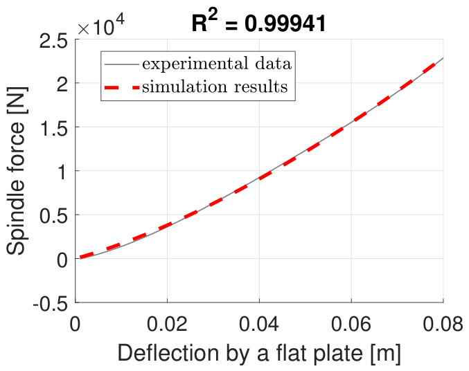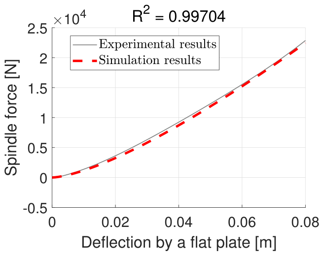In many analytical studies the elasticity of the tire sidewall is modeled as linear radial springs [21,29,31,46]. The linear model is not accurate in certain cases. Consider the application to a flat plate test as shown in Figure 1 [29].

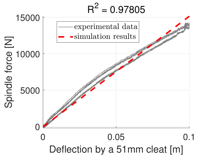
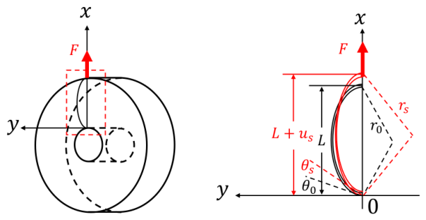
The solid grey line represents the experimental results and the dashed red line represents the simulation. These results are accurate with an R-squared value of 0.999. However, The results of this linear model are not as accurate for a 51 mm cleat test, as shown in Figure 2. The solid grey line indicates the experimental results, including the hysteresis of loading/unloading. The dashed red line indicates the simulation results, which are linear and do not capture the softening of the force-deflection relationship for a cleat. It is clear that the spindle force is nonlinear with respect to the deformation. Such nonlinearity is captured by the linear model because the geometric boundary constraints are changing. That is, the area of the contact patch is increasing as load is applied, leading to an increased number of constrained degrees of freedom (DoF). However, that is not the case for a cleat test where the set of constrained DoF is fixed throughout the testing. Therefore, linear models can accommodate the stiffening effect for the flat plate, but cannot accommodate the softening effect for the cleat. An analysis regarding the sidewall stiffness is therefore necessary. A cross-section of the sidewall is shown in Figure 3. Note that the local reference frame shown in this figure is only to study the sidewall reactions. This frame is not used for the tire model to define directions of forces. The sidewall is of curved shape, resembling the problem of large deformation occurring on an initially curved elastic structure. Note that the x-axis in this figure is the local system attached to the piece of sidewall in discussion, and it should not be confused with the global system attached at the center of the tire. It is assumed to be an elastic beam undergoing no axial deformation along the neutral axis. The curved shape is assumed to be part of a circle with radius $r_0$. The vertical distance between the tread and the wheel at the unloaded situation is denoted as L. The angle between the vertical axis and the tangential line at the connection between the sidewall and the tread/wheel is denoted as ${\theta }_0$. After a vertical tip load F is applied, the tip displacement is denoted as h. The curvature and angle are changed to $r_s$ and ${\theta }_s$.

The relationship between the tip displacement and vertical tip load cannot be assumed to be linear for moderate deflections of a curved beam [43]. Numerical solutions to the problem of an initially curved beam undergoing large deflection has been studied by Kang [47], Mackenzie [48], and Ghuku [49], and show that the relationship is nonlinear. Gao and Liu [50] derived an equation for the structural stiffness, which will be further developed and discussed in Section 3.2. Note that the scope of this work includes moderate deformation, which is significant for a close examination of the sidewall. In developing an explicit relationship between tip deflection and force, it is assumed that the curved sidewall is subjected to bending due to the tip load, and undergoes negligible strain along its neutral axis. In other words the length of the sidewall is held unchanged before and after the deflection.

$$\begin{array}{c}\hfill r_0{\theta }_0=r_s{\theta }_s\end{array}$$

(7)

3. Model Development

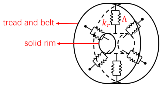
First, models for the contributions of the air pressure, sidewall stiffness, and tread elements are developed from first principles. Next, a general formulation of the nonlinear model is proposed, followed by a numerical solution to the nonlinear system. This includes identifying parameters of the linear part of the model and identifying an admissible nonlinear function and corresponding parameters. A sketch of the model is shown in Figure 4.

The tread and belt are modeled as one elastic beam, supported by a series of radial spring pairs on the solid rim. The beam is discretized into N segments, each representing two degrees of freedom of the model, one radial and one tangential. Each beam segment is connected to the rim by a pair of radial springs, one representing the sidewall stiffness which is denoted as $k_r$ while the other represents the contribution from the inflation pressure, which is denoted as $\mathsf{\Lambda }$. The displacement of each tread and belt segment is measured to evaluate the deformation profile. Forces and deformation equations are then developed for each segment. It is noted that discretizing the elastic ring does not lead to lumping the mass of each segment.

The conventional tire system defined in the SAE J670 standard is adopted in this study. A reference frame following right-hand-rule is constructed such that the origin is the wheel center, x-axis points forward, y-axis parallel to the spindle and z-axis pointing downwards, orthogonal to the ground. Additionally, sign convention in the radial direction is defined such that outwards direction is positive, following a conventional cylindrical system.

3.1. Inflation Pressure

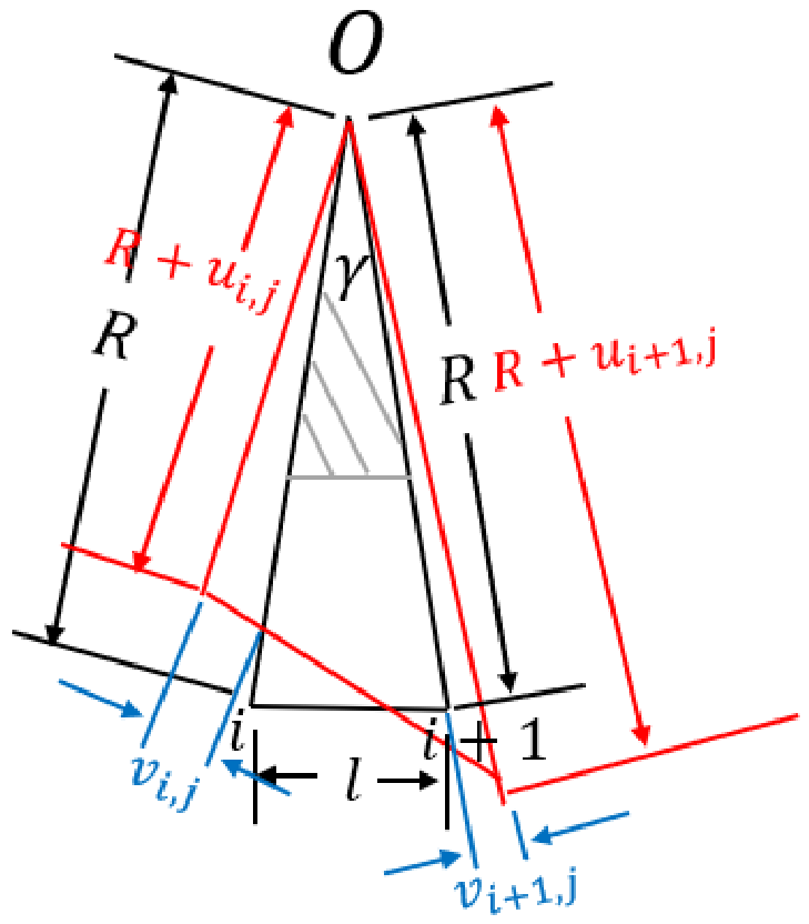
The contribution from inflation pressure to the radial stiffness of the tire is developed in this section. The tire is divided into N small segments. Consider the volume of gas in a segment as illustrated in Figure 5. The sign convention used here is a conventional cylindrical frame, where positive in the radial direction is defined to be outwards, and positive in the circumferential direction is defined to be counter-clockwise. The black lines indicate the undeformed shape of the segment and the red lines indicate the deformed shape. The point O denotes the center of the tire, R denotes its unloaded radius, $u_i$ and $u_{i+1}$ denote the radial displacement of the ith and $i+1$th beam segment, $v_i$ and $v_{i+1}$ denotes the tangential displacement, and $\gamma$ is the included angle where $\gamma =2\pi /N$. The grey shaded area denotes the solid rim at the center that does not contain air, denoted by $S_{grey}$. The ratio of the tire cross-sectional area that is filled with compressed air divided by the total cross-sectional area of the wheel is defined as $\eta$.

$$\begin{array}{c}\hfill {\displaystyle \frac{R^{2}sin\gamma -S_{grey}}{R^{2}sin\gamma }}=\eta \end{array}$$

The work done by the external load to change the volume of the air is modeled by Equation (8).

$$\begin{array}{cc}\hfill W& =-cln{\displaystyle \frac{V_2}{V_1}}\hfill \\ \hfill & =-cln{\displaystyle \frac{{\sum }_i(R+u_i)(R+u_{i+1})sin(\gamma +\frac{v_{i+1}-v_i}{R})-(1-\eta ){\sum }_i{R}^{2}sin\gamma }{\eta {\sum }_i{R}^{2}sin\gamma }}\hfill \\ \hfill & \approx -cln{\displaystyle \frac{\eta N{R}^{2}sin\gamma +2Rsin\gamma {\sum }_{i=1}^N{u}_i+Rcos\gamma {\sum }_{i=1}^N(v_{i+1}-v_i)}{\eta N{R}^{2}sin\gamma }}\hfill \end{array}$$

(8)

This work includes small deflections, defined herein such that terms on the order of ${\epsilon }_{u,i}^2={(u_i/R)}^2<<1$ and ${\epsilon }_{v,i}^2={(v_i/R)}^2<<1$ are negligible. The experimental data used in this work are for a tire with a radius of 0.4 m undergoing radial deflection less than 0.1 m. It is also noticed that the total change in the perimeter is contained by the bead that ${\sum }_{i=1}^N(v_{i+1}-v_i)=0$, therefore it is derived that

$$\begin{array}{c}\hfill W\approx -cln{\displaystyle \frac{\eta NR+2{\sum }_{i=1}^N{u}_i}{\eta NR}}\end{array}$$

(9)

The force applied on one element to change the volume is calculated by Castigliano’s first theorem as given in Equation (10).

$$\begin{array}{cc}\hfill \mathsf{\Lambda }=F_j={\displaystyle \frac{\partial W}{\partial u_j}}& =-c·{\displaystyle \frac{1}{1+\frac{2}{\eta N}{\sum }_i\frac{u_i}{R}}}·{\displaystyle \frac{2}{\eta NR}}\hfill \\ \hfill & ={\displaystyle \frac{-2c}{\eta NR+2{\sum }_i{u}_i}}\hfill \end{array}$$

(10)

In other words, Equation (10) states the force-deformation relationship contributed by the gas. It is shown that the effect of inflation pressure is represented by a term associated with the sum of the deformation profile, ${\sum }_i{u}_i$. Note that the term $\partial W/\partial u_j$ indicates that it corresponds to the jth row on the right-hand side in the matrix form in Equation (1).

Furthermore, the inflation pressure causes the tire to expand radially, which is vital for the load-carrying mechanics of a pneumatic tire [45]. Such radial expansion is denoted as q in this study. The radial expansion sets the sidewall in tension, and this pre-load due to inflation is coupled with the sidewall stiffness developed in Section 3.2, its effect on the model formulation discussed in Section 3.5.

3.2. Nonlinear Sidewall Stiffness

The contribution from the sidewall stiffness to the radial stiffness of the tire is developed in this section. It has been numerically shown in existing studies that the radial stiffness of the tire due to its sidewall is nonlinear. A general form of the force-deformation relationship is written as

$$\begin{array}{c}\hfill F_s(u_s)=k_r{u}_s+f_n(u_s)\end{array}$$

(11)

where the subscript s stands for $sidewall$, the term $k_r$ denotes the linear component of the stiffness and the function $f_n$ denotes the nonlinear component. The nonlinearity can be obtained using the Mooney–Rivlin model [51,52], which is one of the admissible methods to model the elastic sidewall made of hyperelastic materials in finite element studies. In these studies, the sidewall material is characterized by a strain energy density function, which is a linear combination of the strain invariants. An infinitesimal element on the arc, shown in Figure 3 before deformation can be described as

$$\begin{array}{cc}\hfill x& =-r_{0}cos{\theta }_0+r_{0}cos\varphi \hfill \end{array}$$

(12)

$$\begin{array}{cc}\hfill y& ={\displaystyle \frac{L}{2}}+r_{0}sin\varphi \hfill \end{array}$$

(13)

After the deformation the element is moved to

$$\begin{array}{cc}\hfill x^{\prime }& =-r_{s}cos{\theta }_s+r_{s}cos{\displaystyle \frac{{\theta }_s}{{\theta }_0}}\varphi \hfill \\ \hfill y^{\prime }& ={\displaystyle \frac{h+L}{2}}+r_{s}sin{\displaystyle \frac{{\theta }_s}{{\theta }_0}}\varphi \hfill \end{array}$$

The trajectory of an element along the x and y axis is denoted as $u=x^{\prime }-x$ and $v=y^{\prime }-y$. Note that this u here is only to follow the conventional notation in continuum mechanics and should be distinguished from the radial displacement in other parts of the paper.

Taylor series for trigonometric functions and inverse-trigonometric functions are applied to obtain the strain components in the sidewall:

$$\begin{array}{cc}\hfill {ϵ}_x={\displaystyle \frac{\partial u}{\partial x}}& ={\displaystyle \frac{\partial u}{\partial \varphi }}{\displaystyle \frac{\partial \varphi }{\partial x}}\hfill \\ \hfill & ={\displaystyle \frac{r_0\phi -\frac{\phi r_s{\theta }_s^2}{{\theta }_0^2}}{\sqrt{r_0}\sqrt{{\theta }_0^2{r}_0-2x}}}\hfill \\ \hfill {ϵ}_y={\displaystyle \frac{\partial v}{\partial y}}& ={\displaystyle \frac{\partial v}{\partial \varphi }}{\displaystyle \frac{\partial \varphi }{\partial y}}\hfill \\ \hfill & =\left({\displaystyle \frac{{\left(y-\frac{L}{2}\right)}^2}{2r_0^3}}+{\displaystyle \frac{1}{r_0}}\right)\left(r_s\left({\displaystyle \frac{{\theta }_s}{{\theta }_0}}-{\displaystyle \frac{{\phi }^2{\theta }_s^3}{2{\theta }_0^3}}\right)-r_0\left(1-{\displaystyle \frac{{\phi }^2}{2}}\right)\right)\hfill \\ \hfill {\gamma }_{xy}={\displaystyle \frac{\partial u}{\partial y}}& ={\displaystyle \frac{\partial u}{\partial \varphi }}{\displaystyle \frac{\partial \varphi }{\partial y}}\hfill \\ \hfill & =\left({\displaystyle \frac{{\left(y-\frac{L}{2}\right)}^2}{2r_0^3}}+{\displaystyle \frac{1}{r_0}}\right)\left(r_0\phi -{\displaystyle \frac{\phi r_s{\theta }_s^2}{{\theta }_0^2}}\right)\hfill \end{array}$$

Note that the deformation of the cross-section is a planar problem in the local $x-y$ plane, it is assumed that no strain occurs in the direction normal to the plane of the sidewall cross-section being considered. Following sign convention in solid mechanics, the strain invariants are denoted as I and the extension ratios along the three axes of the local system are denoted as $\lambda$. The strain invariants are calculated as

$$\begin{array}{cc}\hfill I_1& ={\lambda }_1^2+{\lambda }_2^2+{\lambda }_3^2\hfill \\ \hfill & ={(1+{ϵ}_{11})}^2+{(1+{ϵ}_{22})}^2+1^2\hfill \\ \hfill & ={ϵ}_x^2+{ϵ}_y^2+{\displaystyle \frac{1}{2}}{\gamma }_{xy}^2+2{ϵ}_x+2{ϵ}_y+3\hfill \\ \hfill & ={\displaystyle \frac{{\left({(L-2y)}^2+8r_0^2\right)}^2{\left({\theta }_0^3{r}_0\left({\phi }^2-2\right)+r_s{\theta }_s\left(2{\theta }_0^2-{\phi }^2{\theta }_s^2\right)\right)}^2}{256{\theta }_0^6{r}_0^6}}\hfill \\ \hfill & +{\displaystyle \frac{\left({(L-2y)}^2+8r_0^2\right)\left({\theta }_0^3{r}_0\left({\phi }^2-2\right)+r_s{\theta }_s\left(2{\theta }_0^2-{\phi }^2{\theta }_s^2\right)\right)}{8{\theta }_0^3{r}_0^3}}\hfill \\ \hfill & +0.5{\left({\displaystyle \frac{{(L-2y)}^2}{8r_0^3}}+{\displaystyle \frac{1}{r_0}}\right)}^2{\left(r_0\phi -{\displaystyle \frac{\phi r_s{\theta }_s^2}{{\theta }_0^2}}\right)}^2+{\displaystyle \frac{{\left(r_0\phi -\frac{\phi r_s{\theta }_s^2}{{\theta }_0^2}\right)}^2}{r_0\left({\theta }_0^2{r}_0-2x\right)}}\hfill \\ \hfill & -{\displaystyle \frac{2\left(r_0\phi -\frac{\phi r_s{\theta }_s^2}{{\theta }_0^2}\right)}{\sqrt{r_0}\sqrt{{\theta }_0^2{r}_0-2x}}}+3\hfill \end{array}$$

(14)

$$\begin{array}{cc}\hfill I_2& ={\lambda }_1^2{\lambda }_2^2+{\lambda }_2^2{\lambda }_3^2+{\lambda }_1^2{\lambda }_3^2\hfill \\ \hfill & ={\lambda }_1^2{\lambda }_2^2+{\lambda }_2^2+{\lambda }_1^2\hfill \\ \hfill & ={\left((1+{ϵ}_{11})(1+{ϵ}_{22})\right)}^2+I_1-1\hfill \\ \hfill & ={({ϵ}_x+{ϵ}_y-{\displaystyle \frac{1}{4}}{\gamma }_{xy}^2)}^2+I_1-1\hfill \\ \hfill & =\left\{{\displaystyle \frac{\left({(L-2y)}^2+8r_0^2\right)\left({\theta }_0^3{r}_0\left({\phi }^2-2\right)+r_s{\theta }_s\left(2{\theta }_0^2-{\phi }^2{\theta }_s^2\right)\right)}{16{\theta }_0^3{r}_0^3}}\right.\hfill \\ \hfill & {\left.-{\displaystyle \frac{1}{4}}{\left({\displaystyle \frac{{(L-2y)}^2}{8r_0^3}}+{\displaystyle \frac{1}{r_0}}\right)}^2{\left(r_0\phi -{\displaystyle \frac{\phi r_s{\theta }_s^2}{{\theta }_0^2}}\right)}^2-{\displaystyle \frac{\left(r_0\phi -\frac{\phi r_s{\theta }_s^2}{{\theta }_0^2}\right)}{\sqrt{r_0}\sqrt{{\theta }_0^2{r}_0-2.x}}}\right\}}^2\hfill \\ \hfill & +I_1\hfill \end{array}$$

(15)

Note that the arc length of the sidewall is held as constant. Taylor series for $sin\theta$ is applied to solve for $\theta$ as a function of h as

$$\begin{array}{cc}\hfill & \left\{\begin{array}{cc}\hfill r_0{\theta }_0& =r_s{\theta }_s\hfill \\ \hfill sin{\theta }_s& ={\displaystyle \frac{L+h}{2r_s}}\hfill \end{array}\right.\hfill \end{array}$$

(16)

$$\begin{array}{cc}\hfill \Rightarrow & {\theta }_s^2=6-3{\displaystyle \frac{h+L}{l_s}}\hfill \end{array}$$

(17)

Mooney-Rivlin model [51] states that the strain energy density is a linear combination of the strain invariants:

$$\begin{array}{c}\hfill W_d=C_{10}(I_1-3)+C_{20}(I_2-3)\end{array}$$

(18)

where $C_{10}$ and $C_{20}$ are constant parameters of the model. The total strain energy due to deformation is therefore

$$\begin{array}{cc}\hfill U& ={\int }_{\mathsf{\Omega }}{C}_{10}(I_1-3)+C_{20}(I_2-3)dV\hfill \end{array}$$

An accurate solution of the strain eneryg can be obtained by substituting Equations (12)–(15) and (17) into Equation (18).

$$\begin{array}{c}\hfill U={\int }_{-{\theta }_0}^{{\theta }_0}\left(C_{10}(I_1(\varphi )-3)+C_{20}(I_2(\varphi )-3)\right)R_{0}d\varphi \end{array}$$

Hamilton’s principal states that the tip load can be calculated by taking a partial derivative of U w.r.t h. The end result takes the form of

$$\begin{array}{c}\hfill F_{tip}={\displaystyle \sum _{i=1}^6}{\alpha }_i{h}^{i/2}\end{array}$$

where each ${\alpha }_i$ is a coefficient involving $C_{10}$, $C_{20}$, ${\theta }_0$, $R_0$ and L.

The nonlinearity has also been studied analytically by Liu and Gao [50]. The structural stiffness is developed by Gao and Liu [50] as

$$\begin{array}{c}\hfill k_r={\displaystyle \frac{2E_s{A}_s\theta }{l_s(2\theta +sin2\theta )}}+{\displaystyle \frac{2E_s{I}_s{\theta }^3}{l_s^3(4\theta +2\theta cos2\theta -3sin2\theta )}}+{\displaystyle \frac{2G_s{A}_s\theta }{l_s(2\theta -sin2\theta )}}\end{array}$$

(19)

Equation (19) can be further developed to explore the nonlinearity due to the changes in h and $\theta$. Taylor series for trigonometric functions are applied to rewrite it as

$$\begin{array}{c}\hfill k_r=C_1{\displaystyle \frac{120}{480-160{\theta }^2+32{\theta }^4}}+C_2{\displaystyle \frac{15}{8{\theta }^2}}+C_3{\displaystyle \frac{15}{20{\theta }^2-4{\theta }^4}}\end{array}$$

(20)

where $C_i$ are the lumped constant coefficients involving the material and geometric constants.

$$\begin{array}{cc}\hfill C_1& ={\displaystyle \frac{2E_s{A}_s}{l_s}}\hfill \\ \hfill C_2& ={\displaystyle \frac{2E_s{I}_s}{l_s^2}}\hfill \\ \hfill C_3& ={\displaystyle \frac{2G_s{A}_s}{l_s}}\hfill \end{array}$$

Plug Equation (17) into Equation (20) to obtain

$$\begin{array}{c}\hfill \begin{array}{cc}\hfill k_r& ={\displaystyle \frac{3C_1}{7}}{\displaystyle \frac{1}{1-(-s_1^2)}}+{\displaystyle \frac{5C_2}{16}}{\displaystyle \frac{1}{1-s_2}}+{\displaystyle \frac{-3C_3}{5}}{\displaystyle \frac{1}{1-s_3^2}}\hfill \\ \hfill s_1& ={\displaystyle \frac{14\sqrt{2}-12\sqrt{2}\frac{h+L}{l_s}}{2\sqrt{70}}}\hfill \\ \hfill s_2& ={\displaystyle \frac{1}{2}}{\displaystyle \frac{h+L}{l_s}}\hfill \\ \hfill s_3& ={\displaystyle \frac{7}{5}}-{\displaystyle \frac{6}{5}}{\displaystyle \frac{h+L}{l_s}}\hfill \end{array}\end{array}$$

(21)

Note that within the scope of this study and the geometric constraints,

$$\begin{array}{c}\hfill 0<|h|<{\displaystyle \frac{1}{2}}L<L<l_s,{\displaystyle \frac{2}{\pi }}<{\displaystyle \frac{L}{l_s}}<1\end{array}$$

Therefore,

$$\begin{array}{cc}\hfill 0.6366& <{\displaystyle \frac{h+L}{l_s}}<1.5\hfill \\ \hfill \Rightarrow -0.3381& <s_1<0.5376\hfill \\ \hfill -0.75& <s_2<-0.3183\hfill \\ \hfill -0.4& <s_3<0.6361\hfill \end{array}$$

and the power series

$$\begin{array}{c}\hfill {\displaystyle \frac{1}{1-x}}=\sum _{i=0}{x}^i,|x|<1\end{array}$$

can be applied to rewrite Equation (21) to move the unknown value of h from the denominator to the numerator.

$$\begin{array}{cc}\hfill k_r& ={\displaystyle \frac{3C_1}{7}}\sum _{i=0}{\left(-s_1^2\right)}^i+{\displaystyle \frac{5C_2}{16}}\sum _{i=0}{\left(s_2\right)}^i+{\displaystyle \frac{-3C_3}{5}}\sum _{i=0}{\left(s_3^2\right)}^i\hfill \\ \hfill & =\sum _{i=0}{\alpha }_i{(h+L)}^i\hfill \end{array}$$

where ${\alpha }_i$ denote the coefficients involving material and geometric constants. It is therefore concluded that a power series of radial displacement is capable of capturing the nonlinearity in the sidewall stiffness within the scope of this study.

3.3. Tread and Belt Stiffness

The strain energy of the system includes the bending and shearing in the tread and belt, given in Equation (22).

$$\begin{array}{c}\hfill U=U_b+U_s\end{array}$$

(22)

The subscript b denotes bending and s denotes shearing and the corresponding strain energy is given in Equation (23).

$$\begin{array}{cc}\hfill U_b& ={\displaystyle \frac{1}{2}}\int EI{\left({\displaystyle \frac{d^{2}u}{d{x}^2}}\right)}^{2}dx\hfill \\ \hfill U_s& ={\displaystyle \frac{1}{2}}\int GS{\left({\displaystyle \frac{du}{dx}}-{\displaystyle \frac{v}{R}}\right)}^{2}dx\hfill \end{array}$$

(23)

The local derivatives are replaced by the finite difference scheme, yielding Equation (24).

$$\begin{array}{cc}\hfill U_b& ={\displaystyle \frac{EI}{2l^3}}{\displaystyle \sum _{i=1}^N}{(u_{i+1}-2u_i+u_{i-1})}^2\hfill \\ \hfill U_s& ={\displaystyle \frac{GS}{8l^3}}{\displaystyle \sum _{i=1}^N}{(u_{i+1}-u_{i-1}-{\displaystyle \frac{2l}{R}}{v}_i)}^2\hfill \end{array}$$

(24)

Castigliano’s first theorem is applied to the finite difference approximation of local derivatives, yielding Equation (25).

$$\begin{array}{cc}\hfill F_i^{(u)}& ={\displaystyle \frac{\partial (U_b+U_s)}{\partial u_i}}\hfill \\ \hfill & ={\displaystyle \frac{\partial }{\partial u_i}}\left[{\displaystyle \frac{EI}{2l^3}}{\displaystyle \sum _{i=1}^N}{(u_{i+1}-2u_i+u_{i-1})}^2+{\displaystyle \frac{GS}{8l}}{\displaystyle \sum _{i=1}^N}{(u_{i+1}-u_{i-1}-{\displaystyle \frac{2l}{R}}{v}_i)}^2\right]\hfill \\ \hfill & ={\displaystyle \frac{EI}{l^3}}(u_{i-2}-4u_{i-1}+6u_i-4u_{i+1}+u_{i+2})+{\displaystyle \frac{GS}{4l}}(2u_i-u_{i+2}-u_{i-2})\hfill \\ \hfill & +{\displaystyle \frac{GS}{2R}}(v_{i+1}-v_{i-1})\hfill \\ \hfill F_i^{(v)}& ={\displaystyle \frac{\partial (U_b+U_s)}{\partial u_i}}\hfill \\ \hfill & ={\displaystyle \frac{GSl}{R^2}}{v}_i-{\displaystyle \frac{GS}{2R}}(u_{i+1}-u_{i-1})\hfill \end{array}$$

(25)

Here, $F_i$ is the generalized force applied on the ith DoF attributed to the strain energy in the tread. The material properties and segment geometry are lumped into parameters A and B.

$$\begin{array}{c}\hfill EI=A,GS=B\end{array}$$

(26)

Equation (25) is written in matrix form as

$$\begin{array}{cc}\hfill F_i& =\left[\begin{array}{cccccccc}{\displaystyle \frac{A}{l^3}}-{\displaystyle \frac{B}{4l}}& -{\displaystyle \frac{4A}{l^3}}& {\displaystyle \frac{6A}{l^3}}+{\displaystyle \frac{B}{2l}}& -{\displaystyle \frac{4A}{l^3}}& {\displaystyle \frac{A}{l^3}}-{\displaystyle \frac{B}{4l}}& -{\displaystyle \frac{B}{2R}}& 0& {\displaystyle \frac{B}{2R}}\\ 0& {\displaystyle \frac{B}{2R}}& 0& -{\displaystyle \frac{B}{2R}}& 0& 0& {\displaystyle \frac{Bl}{R^2}}& 0\end{array}\right]{\mathbf{x}}_{\mathbf{i}}\hfill \\ \hfill {\mathbf{x}}_{\mathbf{i}}& ={\left[\begin{array}{cccccccc}{u}_{i-2}& u_{i-1}& u_i& u_{i+1}& u_{i+2}& v_{i-1}& v_i& v_{i+1}\end{array}\right]}^T\hfill \end{array}$$

(27)

where ${\mathbf{x}}_{\mathbf{i}}$ is a vector containing the local displacement field centered at the ith DoF. Note that in Equation (27) the coefficients of the lumped parameters are derived from the central finite difference scheme, with the order of accuracy being 3. A linear model is constructed by applying Castigliano’s first theorem, and a local stiffness matrix is obtained as

$$\begin{array}{c}\hfill {\mathbf{K}}_{local}=\left[\begin{array}{cccccccc}{\displaystyle \frac{A}{l^3}}-{\displaystyle \frac{B}{4l}}& -{\displaystyle \frac{4A}{l^3}}& {\displaystyle \frac{6A}{l^3}}+{\displaystyle \frac{B}{2l}}& -{\displaystyle \frac{4A}{l^3}}& {\displaystyle \frac{A}{l^3}}-{\displaystyle \frac{B}{4l}}& -{\displaystyle \frac{B}{2R}}& 0& {\displaystyle \frac{B}{2R}}\\ 0& {\displaystyle \frac{B}{2R}}& 0& -{\displaystyle \frac{B}{2R}}& 0& 0& {\displaystyle \frac{Bl}{R^2}}& 0\end{array}\right]\end{array}$$

3.4. Global Stiffness Matrix

Recall that the sidewall stiffness has a linear component, modeled here as a radial stiffness, $k_r$. The addition of the radial stiffness contributed by the sidewall gives an updated version of the local stiffness matrix.

$$\begin{array}{c}\hfill {\mathbf{K}}_{local}=\left[\begin{array}{cccccccc}{\displaystyle \frac{A}{l^3}}-{\displaystyle \frac{B}{4l}}& -{\displaystyle \frac{4A}{l^3}}& {\displaystyle \frac{6A}{l^3}}+{\displaystyle \frac{B}{2l}}+k_r& -{\displaystyle \frac{4A}{l^3}}& {\displaystyle \frac{A}{l^3}}-{\displaystyle \frac{B}{4l}}& -{\displaystyle \frac{B}{2R}}& 0& {\displaystyle \frac{B}{2R}}\\ 0& {\displaystyle \frac{B}{2R}}& 0& -{\displaystyle \frac{B}{2R}}& 0& 0& {\displaystyle \frac{Bl}{R^2}}& 0\end{array}\right]\end{array}$$

(28)

The global stiffness matrix is a symmetric circulant matrix,

$$\begin{array}{cc}\hfill {\mathbf{K}}_{global}& =\left[\begin{array}{cc}{\mathbf{K}}^{(\mathbf{uu})}& {\mathbf{K}}^{(\mathbf{uv})}\\ {\mathbf{K}}^{(\mathbf{vu})}& {\mathbf{K}}^{(\mathbf{vv})}\end{array}\right]\hfill \end{array}$$

(29)

$$\begin{array}{c}\hfill \begin{array}{cc}\hfill {\mathbf{K}}^{(\mathbf{uu})}& =toeplitz(\left[\begin{array}{c}{\displaystyle \frac{6A}{l^3}}+{\displaystyle \frac{B}{2l}}+k_r,-{\displaystyle \frac{4A}{l^3}},{\displaystyle \frac{A}{l^3}}-{\displaystyle \frac{B}{4l}},0,\dots ,0,{\displaystyle \frac{A}{l^3}}-{\displaystyle \frac{B}{4l}},-{\displaystyle \frac{4A}{l^3}}\end{array}\right])\hfill \\ \hfill {\mathbf{K}}^{(\mathbf{uv})}& =toeplitz(\left[\begin{array}{c}0,{\displaystyle \frac{B}{2R}},0,\dots ,0,-{\displaystyle \frac{B}{2R}}\end{array}\right])\hfill \\ \hfill {\mathbf{K}}^{(\mathbf{vu})}& ={({\mathbf{K}}^{(\mathbf{uv})})}^T\hfill \\ \hfill {\mathbf{K}}^{(\mathbf{vv})}& =toeplitz(\left[\begin{array}{c}{\displaystyle \frac{Bl}{R^2}},0,\dots ,0\end{array}\right])\hfill \end{array}\end{array}$$

(30)

which corresponds to a global displacement vector

$$\begin{array}{c}\hfill \mathbf{x}={\left[\begin{array}{cccccccc}{u}_1& u_2& \cdots & u_N& v_1& v_2& \cdots & v_N\end{array}\right]}^T\end{array}$$

(31)

Equations (28) and (30) states the local and global stiffness of the model, forming a linear system with the applied loads and displacement field.

3.5. General Form of the Force-Deformation Relationship

In this work the radial deformation, u, is measured from the inflated, but unloaded, shape of the tire. It has been mentioned in Section 2.4 that the radial expansion due to the inflation pressure on one degree of freedom is denoted as q. For the 2D model proposed in this study, q is a constant for all degrees of freedom due to symmetry. A vector that denotes such expansion on all degrees of freedom is therefore a constant vector $\mathbf{q}$, of which all the entries are equal to q. The deformation of a tire is always measured from its inflated but unloaded state, denoted as $\mathbf{u}$. Each of its entries is written as $u_i$ to represent the deformation measured on the $i^{th}$ DoF. The total elastic deformation is the sum of the measured deformation and the pre-expansion:

$$\begin{array}{cc}\hfill {\mathbf{u}}_{\mathbf{total}}& =\mathbf{u}+\mathbf{q}\hfill \\ \hfill \mathbf{u}& =\left[\begin{array}{c}{u}_1\\ u_2\\ ⋮\\ u_N\end{array}\right],\mathbf{q}=\left[\begin{array}{c}q\\ q\\ ⋮\\ q\end{array}\right]\hfill \end{array}$$

When evaluating the elastic force of the system, this sum ${\mathbf{u}}_{\mathbf{total}}$ should be substituted into the equations instead of simply $\mathbf{u}$. After combining the terms associated with inflation pressure in Equation (10) and tire stiffness in Equation (30), the general form of the force-deformation relationship is written as

$$\begin{array}{c}\hfill \mathbf{F}={\mathbf{K}}_{\mathbf{global}}(\mathbf{u}+\mathbf{q})+f_n(\mathbf{u}+\mathbf{q})-\mathsf{\Lambda }\end{array}$$

where $\mathsf{\Lambda }$ is a matrix, of which its entries are equal to ${\displaystyle \frac{2c}{\eta NR+2{\sum }_i{u}_i}}$, as shown in Equation (10). The unloaded tire condition can be verified by setting $\mathbf{u}=0$.

$$\begin{array}{cc}\hfill {\mathbf{F}}_{\mathbf{0}}& ={\mathbf{K}}_{\mathbf{globalq}}+f_n(\mathbf{q})-{\mathsf{\Lambda }}_{\mathbf{0}}\hfill \\ \hfill {(F_0)}_i& =k_{r}q+f_n(q)-{\displaystyle \frac{2c}{\eta NR}}\hfill \end{array}$$

where $(k_{r}q+f_n(q))$ equals the force exerted by inflation pressure on one beam segment in the unloaded state, given that the deformation due to inflation is uniform. Assume that the air pressure is denoted as $p_0$ in such state and that the lateral thickness of the tire is denoted as T. The tire is divided into N segments then each segment obtains a central angle $\gamma =2\pi /N$.

$$\begin{array}{cc}\hfill k_{r}q+f_n(q)& =p_{0}R\gamma T={\displaystyle \frac{c}{\eta \pi R^{2}T}}·R·{\displaystyle \frac{2\pi }{N}}T={\displaystyle \frac{2c}{\eta NR}}\hfill \\ \hfill \Rightarrow F_0& =0\hfill \end{array}$$

When no load is applied to the inflated tire, the term representing external force is 0. Or, one could interpret the left hand side as the “net force” and move the term derived from inflation pressure from the right hand side to the left as well.

3.6. Numerical Solution with Newton-Raphson Method

Once the forces and deformation equations are constructed, it is desired to be solved. For this study the exact solution to a high order nonlinear system could be hard to obtain, therefore a numerical solution is obtained. The function describing the system dynamics can be written as

$$\begin{array}{cc}\hfill \left[\begin{array}{c}\mathbf{F}\\ \mathbf{0}\end{array}\right]& =\left[\begin{array}{cc}{\mathbf{K}}_{\mathbf{cc}}& {\mathbf{K}}_{\mathbf{cu}}\\ {\mathbf{K}}_{\mathbf{uc}}& {\mathbf{K}}_{\mathbf{uu}}\end{array}\right]\left[\begin{array}{c}{\mathbf{x}}_{\mathbf{c}}+{\mathbf{q}}_{\mathbf{c}}\\ {\mathbf{x}}_{\mathbf{u}}+{\mathbf{q}}_{\mathbf{u}}\end{array}\right]+\left[\begin{array}{c}{f}_n({\mathbf{x}}_{\mathbf{c}}+{\mathbf{q}}_{\mathbf{c}})\\ f_n({\mathbf{x}}_{\mathbf{u}}+{\mathbf{q}}_{\mathbf{u}})\end{array}\right]+\left[\begin{array}{c}{\mathsf{\Lambda }}_{\mathbf{c}}\\ {\mathsf{\Lambda }}_{\mathbf{u}}\end{array}\right]\hfill \end{array}$$

(32)

$$\begin{array}{cc}\hfill \mathsf{\Lambda }& ={\displaystyle \frac{-2c}{\eta NR+2{\sum }_i{x}_i}}\hfill \end{array}$$

(33)

where $\mathbf{x}$ is rearranged such that the entries of its upper part correspond to the constrained DoFs (denoted by the subscript c, or in other words, the DoFs that are in the contact patch. The entries of its lower part correspond to the unconstrained DoFs (denoted by the subscript u), or in other words, the DoFs that are outside of the contact patch. The terms ${\mathbf{q}}_{\mathbf{c}}$ and ${\mathbf{q}}_{\mathbf{u}}$ are both vectors with all of their entries equal to q or 0, depending on the specific alignment with the rearranged displacement vector such that only radial displacements u are added with q. Together they can form the vector $\mathbf{q}$ which denotes the radial expansion due to inflation pressure. The subscripts are merely to align with other terms in the matrix operations. Vectors ${\mathsf{\Lambda }}_c$ and ${\mathsf{\Lambda }}_u$ are the same case, where all of their entries are equal to $\mathsf{\Lambda }$ and the subscripts are for alignment. The function written in this form so that the unknowns can be solved by parts with adoption of Guyan’s reduction [42]. A function is defined as:

$$\begin{array}{c}\hfill {\mathbf{F}}_{\mathbf{u}}={\mathbf{K}}_{\mathbf{uc}}({\mathbf{x}}_{\mathbf{c}}+{\mathbf{q}}_{\mathbf{c}})+{\mathbf{k}}_{\mathbf{uu}}({\mathbf{x}}_{\mathbf{u}}+{\mathbf{q}}_{\mathbf{u}})+f_n({\mathbf{x}}_{\mathbf{u}}+{\mathbf{q}}_{\mathbf{u}})+{\mathsf{\Lambda }}_u\end{array}$$

where the root of ${\mathbf{F}}_{\mathbf{u}}=\mathbf{0}$ is the desired ${\mathbf{x}}_{\mathbf{u}}$ with which the spindle force and the deformation profile are obtained.

One of the problems with introducing nonlinear functions in the model is obtaining the roots. Fortunately, it is observed in Figure 2 that although the linear solution is not accurate, it does not significantly deviates from the nonlinear solution. Therefore, Newton–Raphson method can be adopted to obtain ${\mathbf{x}}_{\mathbf{u}}$, given the value of ${\mathbf{x}}_{\mathbf{c}}$. The linear solution is used as the starting point:

$$\begin{array}{cc}\hfill \mathbf{0}& ={\mathbf{K}}_{\mathbf{uc}}({\mathbf{x}}_{\mathbf{c}}+{\mathbf{q}}_{\mathbf{c}})+{\mathbf{k}}_{\mathbf{uu}}({\mathbf{x}}_{\mathbf{u}}^{(\mathbf{0})}+{\mathbf{q}}_{\mathbf{u}})\hfill \\ \hfill {\mathbf{x}}_{\mathbf{u}}^{(\mathbf{0})}& =-{\mathbf{K}}_{\mathbf{uu}}^{-\mathbf{1}}{\mathbf{K}}_{\mathbf{uc}}({\mathbf{x}}_{\mathbf{c}}+{\mathbf{q}}_{\mathbf{c}})-{\mathbf{q}}_{\mathbf{u}}\hfill \end{array}$$

Newton–Raphson method states that the approximated root of the sth iteration is obtained as

$$\begin{array}{c}\hfill {\mathbf{x}}_{\mathbf{u}}^{(\mathbf{s})}={\mathbf{x}}_{\mathbf{u}}^{(\mathbf{s}-\mathbf{1})}-{\mathbf{J}}^{-\mathbf{1}}{\mathbf{F}}_{\mathbf{u}}({\mathbf{x}}_{\mathbf{u}}^{(\mathbf{s}-\mathbf{1})})\end{array}$$

(34)

The Jacobian of ${\mathbf{F}}_{\mathbf{u}}$ is obtained as

$$\begin{array}{cc}\hfill \mathbf{J}& ={\mathbf{k}}_{\mathbf{uu}}\hfill \\ \hfill & +diag\left(\left[\begin{array}{ccccc}{f}_n^{\prime }(x_1^{(s-1)}+q)& f_n^{\prime }(x_2^{(s-1)}+q)& f_n^{\prime }(x_3^{(s-1)}+q)& \cdots & f_n^{\prime }(x_N^{(s-1)}+q)\end{array}\right]\right)\hfill \\ \hfill & +\left[{\displaystyle \frac{4c}{{(\eta NR+2{\sum }_i{x}_i^{(s-1)})}^2}}\right]\hfill \end{array}$$

(35)

where $x_i^{(s-1)}$ denotes the ith entry in the column vector ${\mathbf{x}}_{\mathbf{u}}^{(\mathbf{s}-\mathbf{1})}$. The last term is a square matrix of the same size as ${\mathbf{K}}_{\mathbf{uu}}$, and all of its entries are equal to the term in parentheses. Within the scope of this study, the convergence criterion can be set to be the maximum element-wise step in the displacement vector. For example, the iterative process terminates once the maximum element-wise step in the displacement vector is less than 0.1 mm.

4. Experimental Model Calibration and Simulation Results

Two sets of experimental data are used in this study. Part of each set of data is used for calibration of the model, and part of the data is used to validate the proposed model.

The first set was provided by Prof. Els from University of Pretoria to the Vehicle Terrain Performance Lab led by Prof. Ferris at Virginia Tech. The tire tested was the Continental Conti-Trac AT235/85 R16 (Continental AG, Hannover, Germany). The tire was mounted to a rigid spindle and a loading machine slowly pressed a flat plate and cleats of different sizes onto the tire in multiple iterations. A displacement transducer and a force transducer were embedded in the loading machine to measure the normal force applied to the tire as well as radial deformation in a quasi-static situation. This set of data will be used to validate the model in terms of predicting normal force.

The other data set was collected in the Terramechanics, Multibody and Vehicle Systems Laboratory led by Prof. Sandu at Virginia Tech. The tire tested was a Michelin P225/60 R16 standard reference test tire (SRTT) (Michelin, Clermont-Ferrand, France). The tire was mounted to a LW-2T-20K wheel force transducer system manufactured by Michigan Scientific Corporation (Charlevoix, MI, USA). The transducer was further installed on a loading machine to press the tire onto a rigid surface. A Bosch GLM 15 laser measure was attached to the force transducer to measure the displacement, and a TekScan Model 7101 (TekScan, Norwood, MA, USA) pressure pad was placed between the tire and the rigid surface to measure the pressure distribution. This set of data will be used to validate the model in terms of predicting normal pressure distribution in the longitudinal direction.

In previous derivations many material properties are involved, including Young’s modulus E, shear modulus G, and geometric constants including the bending moment of inertia I. Note that a pneumatic tire is a highly complex structure, composed of different layers and parts made from various materials embedded in different sections of the tire. Analytical models including the brush model, flexible ring model, elastic string model, and the model proposed in this paper, aggregate all the different materials into one to replace a computationally expensive finite element model. Upon reviewing existing studies utilizing FEM, it’s observed that most models do not fully capture the tire’s intricate structure. Researchers, such as Chae [15], have proposed detailed models by segmenting the tire into multiple layers, yet these models still lack the complexity of a real tire. Additionally, certain structural aspects, such as the interlaced and embedded structure of the bead, are often not represented in isolation within these models. All discussed parameters are lumped model parameters, representing properties of the entire tire.

The calibration process of the model, as well as comparisons between the simulation results and experimental results are demonstrated in this section.

4.1. Spindle Force Prediction

4.1.1. Calibration

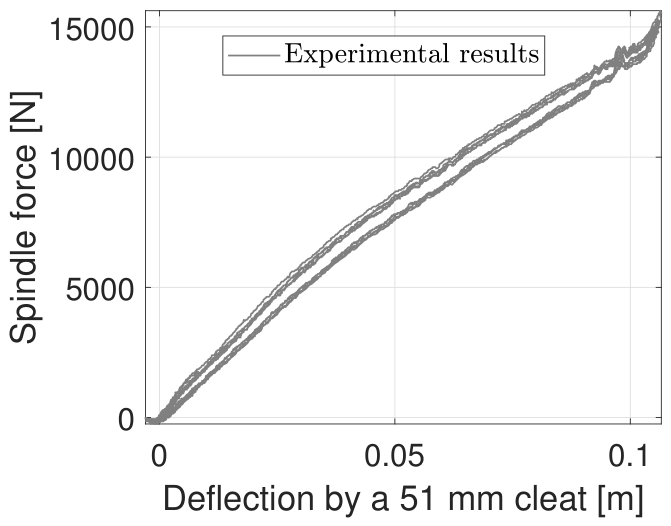
Two groups of experimental data of the Continental Conti-Trac AT 235/85 R16 tire were used for calibration. The first group was collected when the loading machine pressed a 51 mm cleat onto the tire. Figure 6 shows the original experimental data from a 51 mm cleat test.

The curvature changes significantly beyond 0.1m deformation. This is likely due to an abrupt change in the loading conditions within the complicated multi-layer structure of the tire. The scope of this work includes only small to moderate deformation and 0.1 m marks the end of referred data. The abrupt change of spindle force for deformation greater than 0.1 m is omitted. The proposed model also includes no dampers, hence the hysteresis effect is not reflected by the model. The second data group was collected when the loading machine pressed a rigid flat plate onto the tire.

To obtain the values of model parameters, an interior-point optimization algorithm is adopted. The objective is to minimize the sum of squares of the difference between the simulated spindle force and the experimental data from the two data groups mentioned earlier, given the applied deformation.

It has been mentioned in Section 2.5 that a power series can be used to approximate the nonlinear sidewall stiffness. In this example, a 3rd order polynomial is used to capture the nonlinearity.

$$\begin{array}{c}\hfill F(u)={\alpha }_{1}u+{\alpha }_2{u}^2+{\alpha }_3{u}^3\end{array}$$

(36)

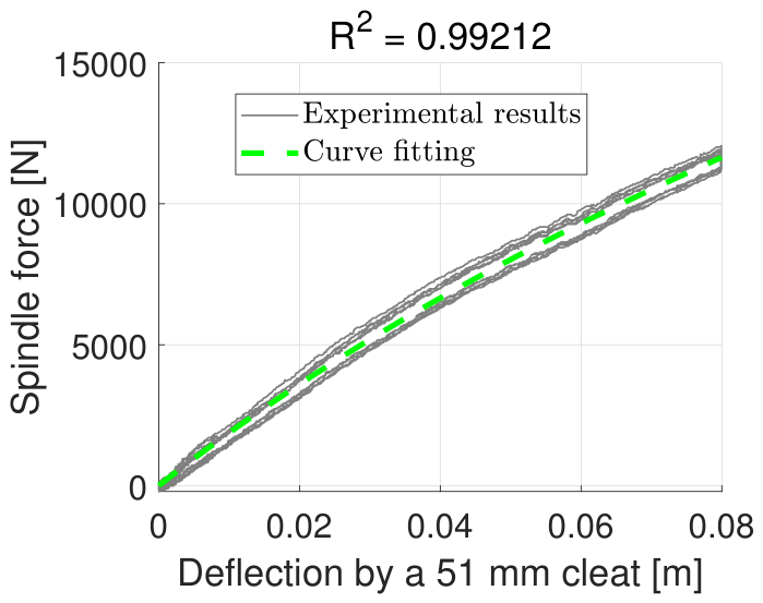
The validation of the 3rd order polynomial is based on the data of the 51 mm cleat test. A 3rd order polynomial is fit to the data of interest, as is shown in Figure 7.

The grey line denotes the original data of interest. The green line is obtained through a 3rd order polynomial curve fit, which fits the experimental data with a coefficient of determination greater than 0.99. This example demonstrates that the stiffness of the tire can be approximated with a polynomial. Furthermore, it suggests that the nonlinear aspect of the solution can also be adequately approximated with polynomials, which is utilized in the discussion of nonlinear stiffness.

The elastic beam which resembles the tread and belt component is discretized into 480 segments. Each segment obtains a radial displacement and a circumferential displacement in the displacement vector. It is pointed out that one DoF denotes one displacement component, rather than one complete segment. The model parameters identified by the calibration process are listed below:

$$\begin{array}{cc}\hfill A& =5.366e4\hfill \\ \hfill B& =1.2563e5\hfill \\ \hfill q& =0.0034\hfill \\ \hfill {\alpha }_1& =2.4064e3\hfill \\ \hfill {\alpha }_2& =4.8028e4\hfill \\ \hfill {\alpha }_3& =-7.8519e4\hfill \end{array}$$

where A and B are the parameters contributed from the tread and belt stiffness, derived in Section 3.3. Parameter q is the parameter contributed from the inflation pressure, derived in Section 2.4. The $\alpha$ parameter set represents the contribution from the sidewall stiffness, derived in Section 2.5. 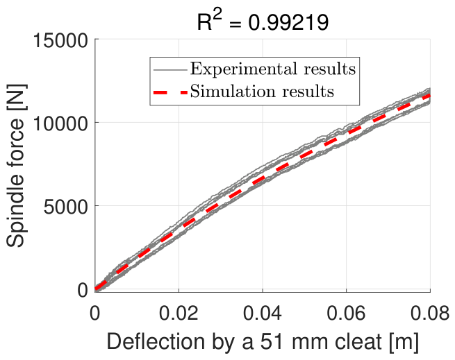The constraints applied onto the parameters are that the values of A, B, q should all be greater than 0, and that ${\alpha }_{1}u+{\alpha }_2{u}^2+{\alpha }_3{u}^3\le 0$ for all $-0.1\le u\le 0$, to comply with the physical boundaries associated with the parameters. Note that the tire consists of a complicated multi-layer structure, and all of these variables are essentially “equivalent” material properties. In other words, the multiple materials of which the tire is made are lumped together and treated as composite materials. This is a common approach for empirical, semi-empirical, and analytical tire models that reduce the numbers of unknowns and equations. The accuracy of the model is achieved by developing the model in a deliberate way so that it reflects tire physics and mechanics despite the simplifications. In other words, these parameters are equivalent parameters to represent lumped physical behaviors of the tire, and they should not be treated as the real experimental measurements due to their approximation nature. After identifying the parameters in Equation (36), the model matches the smoothed experimental data to an $R^2$ value of $0.99$, as shown in Figure 8. Note that the quadratic stiffness term defined in Equation (36) has the same $R^2$ value of 0.99 as the cubic polynomial fit shown in Figure 7 (to the second decimal place).

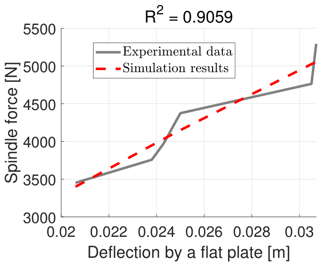
Comparing Figure 8 with Figure 2 shows the necessity of including this nonlinearity. The linear fit shown in Figure 2 does not include any of the softening effects exhibited by the experimental data. In contrast, the nonlinear response exhibited in Figure 8 clearly does and with an accuracy equivalent to the best curve fit that could be attained with a cubic polynomial. Meanwhile, the calibration also involves the flat plate test and the results are shown in Figure 9:

4.1.2. Simulation Results

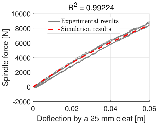
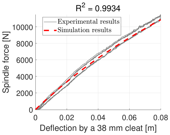
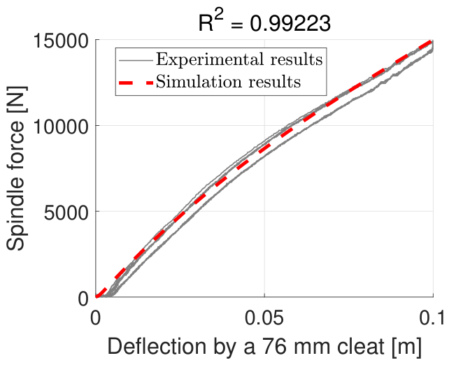
The lumped parameters: A, B, q, ${\alpha }_1$, ${\alpha }_2$ and ${\alpha }_3$ are used, without alteration, in the simulations on a 25 mm, 38 mm, 76 mm, and 100 mm cleat. During the experiment the loading machine pressed these four cleats onto the tire, respectively. The simulation results are compared with experimental results in the following context.

First, consider the results of the cleat test for cleats that are smaller than the 51 mm cleat used for parameter identification. The 25 mm cleat results are shown in Figure 10. The predicted curve follows the upper part of the experimental data for small deflection, then moves down to the lower part for relatively greater deflection with an $R^2$ value greater than 0.99.

The same pattern is also shown in the results for 38 mm cleat test, as shown in Figure 11.

The results for 76 mm cleat test demonstrate a different pattern that the predicted curve sticks to the upper part of the experimental data, as shown in Figure 12.

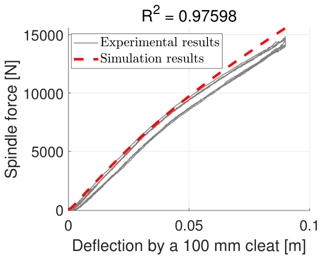
Both cases of 38 mm cleat and 76 mm cleat give coefficients of determination greater than 0.99. The prediction for 100 mm cleat demonstrates a similar pattern as the 76 mm cleat for small deflection, then for large deflection the model overestimates the spindle force with a maximum error of roughly 6%, as shown in Figure 13. The $R^2$ value for the 100 mm cleat test is greater than 0.97.

A potential cause for the inaccuracy is the omission of lateral behaviors, which would require a 3D model. For a 2D model, assuming a contact line between the tire and ground or the cleat implies that the contact patch is rectangular. However, that is generally not the case for a real tire whose contact patch is often wider in the center and narrower beneath the sidewalls. Such inconsistency between a 2D model and a real tire becomes significant when the cleat is wide and provides enough area for the contact patch to develop.

4.2. Normal Pressure Distribution Prediction

4.2.1. Calibration

The data set of the SRTT was used to validate the model in terms of pressure distribution. The model is calibrated using the spindle force, as shown in Figure 14:

The elastic beam resembling the tread and belt component is discretized into 480 segments. The model parameters identified by the calibration process are listed below:

$$\begin{array}{c}\hfill \begin{array}{cc}\hfill A& =1.0134e5\hfill \\ \hfill B& =6.8823e3\hfill \\ \hfill q& =4.6138e-4\hfill \\ \hfill {\alpha }_1& =5.9075e3\hfill \\ \hfill {\alpha }_2& =1.0307e5\hfill \\ \hfill {\alpha }_3& =51.3358\hfill \end{array}\end{array}$$

(37)

4.2.2. Simulation Results

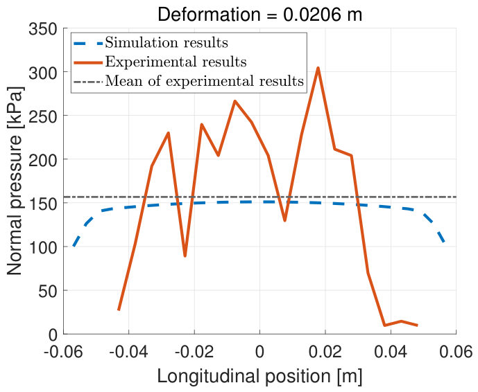
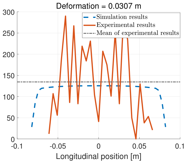
The same parameter set is used to predict the normal pressure distribution over the contact patch, in the longitudinal direction. The results are shown in Figure 15 and Figure 16.

It is pointed out that the pressure distribution is compared in the longitudinal direction at the center of the contact patch. Therefore, this comparison does not represent a validation of the complete 2D pressure field. The pressure measurements are not used during the parameter identification of the SRTT. The parameters are identified with the spindle force first, then used without alteration to predict the pressure distribution.

Note that the normal pressure distribution of a real tire varies in the lateral direction. However, the model proposed in this study is a 2D model so the prediction cannot reflect such variation. The simulation results are compared with the pressure measured at the center of the contact patch.

The zig-zag pattern in the experimental data is caused by the grooves in the tread. The tread material inside of a groove is barely in touch with the pressure pad, causing a local minimum. On the other hand, the tread material of the raised part carries all loads in its adjacency, leading to local peaks. The simulation results tend to overestimate the size of the contact patch by roughly 18% due to the omission of tangential movements of the tread segments, and the simulated pressure value goes through the experimental curves as a mean value of the local minima and local peaks. The simulation results of normal pressure increase rapidly near the entrance and the exit of the contact patch, with very small variations in the central part. In Figure 15 the simulation results are 16–22% smaller than the experimental data in the central part. Figure 16 demonstrates a similar pattern but the simulation results are greater than the experimental data at the central part of the contact patch, roughly 9% at the peak.

Concerns may rise regarding the net normal force. For example, in both figures it appears that the sum of the simulation results is smaller than that of the experimental results, but the calibration process states that there is little difference between the simulated and experimental net normal force. This is due to the fact that the 2D model fails to capture the tire behaviors in the lateral direction. The experimental curve in Figure 15 is measured at the center of the contact patch. At the outer or inner edge of the contact patch, the longitudinal length is much smaller than the center, offering much less net local normal force. The 2D model, however, fails to capture this phenomenon due to its inherent disadvantage and “assumes” that the contact patch is rectangular. In other words, the underestimations at the center are “compensated” by over-estimations at the edge. The signature of the model is that the predicted normal pressure is close to the mean value of the experimental pressure at the center of the contact patch. Investigating the behaviors in the lateral direction calls for the development of a 3D tire model, which will be proposed by the researcher in another study.

5. Conclusions

This study proposes a 2D tire modeling technique, which employs an analytical approach based on beam theory and numerical approximations. The parameters of the model are deliberately chosen to reflect the tire’s physical properties as well as the load carrying mechanism. Additionally, the study offers justifications for common assumptions made in analytical models, particularly regarding sidewall stiffness and inflation pressure, aimed at simplifying equations within a certain scope. The model is capable of providing predictions of the spindle force and the pressure distribution over the contact patch with less computational effort compared to an FEM. The comparison between the prediction and experimental data shows high coefficients of determination. It is also capable of capturing the characteristics of the normal pressure distribution over the contact patch, proven useful for vehicle handling studies. It could therefore be adopted in the tire development process, as well as in vehicle dynamics studies.

The computational time is significantly short compared to finite element models. It generally takes less than 1.5 s to calculate the spindle force and pressure distribution with MATLAB 2022a installed on an Intel i7 processor. Published FRM tire models generally take hours to complete a loading simulation, with [53] being a good example where the solving process is optimized to reduce computational time.

The model can be further developed to 3D, with the tread and belt component evaluated by a 3D analytical model. For example, there are studies suggesting that a circular cylindrical shell can be used to model a tire. Another potential improvement is to include dampers in the model to resemble the hysteresis effect.

Other possible model extensions are to incorporate friction (e.g., LuGre model) and to evaluate the traction force based on the normal pressure and vertical load results. It can also be integrated into vehicle dynamics studies to provide vertical load given the terrain shape.