Article

A Husimi Phase-Space Approach to a Driven–Dissipative Quantum Field at Finite Temperature

by
Marco A. García-Márquez
*,
Irán Ramos-Prieto
,
Francisco Soto-Eguibar
and
Héctor M. Moya-Cessa
*
Instituto Nacional de Astrofísica, Óptica y Electrónica, Calle Luis Enrique Erro No. 1, Santa María Tonantzintla, Puebla 72840, Mexico
*
Authors to whom correspondence should be addressed.
Dynamics 2026, 6(3), 26; https://doi.org/10.3390/dynamics6030026
Submission received: 26 June 2026 / Revised: 20 July 2026 / Accepted: 21 July 2026 / Published: 23 July 2026

Abstract

We investigate the dynamics of a driven quantum field coupled to a finite-temperature reservoir. The corresponding master equation is solved using superoperator techniques, yielding an analytical expression for the density operator. To obtain a compact and physically transparent description of the dynamics, we adopt a phase-space representation based on the Husimi Q-function. For an initially coherent state, we derive a closed-form Gaussian expression for the Husimi Q-function whose stationary limit corresponds to a displaced thermal state. This approach also enables an analytical study of quantum-interference dynamics for an initial superposition of coherent states. Furthermore, we derive the corresponding Fokker–Planck equation for the Husimi Q-function and obtain closed-form expressions for relevant statistical quantities, including the mean photon number, the photon-number standard deviation, and the Mandel parameter. We also investigate the Wehrl and linear entropies, which quantify the loss of phase-space information and purity induced by the thermal environment. The framework provides a complete analytical characterization of the phase-space dynamics, photon statistics, and entropic properties of driven–dissipative quantum fields while avoiding the explicit manipulation of the density operator.

1. Introduction

The interaction between quantum systems and their environment is a central topic in quantum physics since realistic systems cannot be completely isolated. Coupling to the surroundings induces dissipative dynamics, leading to decoherence and thermalization and thus reducing quantum features, such as coherence and entanglement [1,2]. Among open quantum systems, driven–dissipative quantum fields play a prominent role. In these systems, a quantized field is simultaneously subjected to coherent external driving and to dissipation arising from its coupling to a thermal reservoir. Early studies derived the reduced density operator and the quantum characteristic function for a driven field mode that interacts with a thermal bath [3], obtained exact solutions of the corresponding master equation through iterative methods [4], and later exploited the algebraic structure of the operator space and gauge transformations to construct exact analytical solutions [5]. This interplay leads to nontrivial coherent and incoherent dynamics [6]. The theoretical description of such systems is commonly based on the Lindblad master equation [7]. Analytical solutions for a quantized harmonic oscillator coupled to a thermal reservoir have been extensively studied in the literature and different approaches have been used, such as proposing an ansatz to solve the master equation [8], solving the differential equations that govern the evolution of the elements of the density matrix [9], using functional integrals [10], and, more recently, this problem has been generalized to two interacting quantized fields coupled to thermal reservoirs, giving rise to exact solutions based on effective non-Hermitian Hamiltonians [11], finite-temperature formulations [12], and studies of the dynamics and quantum correlations of interacting coherent states in dissipative cavities [13]. For the single-field problem, superoperator formalisms have also been widely employed [14]. The inclusion of a linear driving term in this context has also been investigated [15].
Although exact analytical solutions can be obtained for driven dissipative oscillators [3,4,5,16], they often involve cumbersome calculations or infinite series expansions, which may obscure the physical interpretation of the underlying dynamics. Alternative approaches leading to more explicit expressions have also been proposed [6]. These considerations motivate the search for formulations that provide a more transparent description of the system.
A particularly powerful approach to the study of dissipative quantum fields is provided by phase-space methods, in which the density operator is represented by a quasiprobability distribution function. For example, the dynamics of a cavity field coupled to a thermal bath has been described in terms of a Fokker–Planck equation for the Husimi Q-function [17], while, in [18], the evolution of a cavity field is studied using the coherent-state expansion of the density operator, namely the Glauber–Sudarshan P-representation. More recently, [19] extended this framework to analyze the dynamics of a cavity field in a squeezed thermal environment.
Such models provide a useful framework for analyzing the statistical properties of the field [8], as well as for studying the effects of dissipation on phase-space interference [2] and for investigating the decay of quantum superpositions of displaced states, such as Schrödinger cat states and displaced thermal states, under interaction with a thermal reservoir [17].
In this work, we examine a driven quantum field that interacts with a finite-temperature reservoir. In Section 2, we present the physical model under consideration and solve the associated master equation analytically using superoperator methods. Even when the initial state is coherent, the resulting solution takes the form of an infinite series. To address this complication, in Section 3, we adopt a phase-space formulation based on the Husimi Q-function, defined by projecting the density operator onto coherent states. Within this setting, our analysis extends earlier treatments by explicitly incorporating the driving term and offering a physically transparent phase-space picture of the dynamics. In particular, we obtain an analytical form of the Husimi function for an initial superposition of coherent states and study how its Gaussian and interference components evolve in the presence of driving, dissipation, and thermal noise. We also derive the corresponding Fokker–Planck equation that governs the time evolution of the Husimi function, enabling a detailed characterization of the field. To situate our approach within standard theoretical frameworks, we emphasize that, because the model is linear and preserves Gaussianity, its dynamics can be directly identified with those of Gaussian quantum channels and the familiar driven damped harmonic oscillator, where the driving term may be removed by a displacement transformation. Accordingly, the long-time relaxation toward a displaced thermal state follows straightforwardly from conventional theory. However, the key benefit of our method is that it provides a direct phase-space toolkit. By working entirely in the Husimi Q-representation, we obtain closed-form analytical expressions for the evolution of nonclassical states, photon-number statistics, and entropic quantities, thereby avoiding the cumbersome infinite-series expansions and operator manipulations that typically arise in density-operator approaches. In Section 4, we investigate the photon statistics of the system by evaluating the mean photon number, its standard deviation, and the Mandel parameter. In Section 5, we explore the entropic features of the system through the Wehrl and linear entropies. Finally, Section 6 contains our main findings and our concluding remarks.

2. Physical Model and Master Equation

The master equation for the density operator ρ ˜ ^ of a quantized field driven by a classical field coupled to a thermal reservoir at finite temperature is given by [4,20]
d ρ ˜ ^ d t = i H ^ , ρ ˜ ^ + γ ( n th + 1 ) L [ a ^ ] ρ ˜ ^ + γ n th L [ a ^ ] ρ ˜ ^ ,
where H ^ = ω n ^ + ξ a ^ e i ω t + a ^ e i ω t is the Hamiltonian that describes the interaction between the fields, with n ^ = a ^ a ^ the number operator, a ^ and a ^ the annihilation and creation operators, ω is the frequency of the quantized field and ξ represents the strength of the coupling to the external source oscillating resonantly at frequency ω . The dissipative part is described by Lindblad superoperators L [ c ^ ] ρ ^ = 2 c ^ ρ ^ c ^ ( c ^ c ^ ρ ^ + ρ ^ c ^ c ^ ) , with c ^ = a ^ , a ^ , where γ is the dissipation rate and n th is the average number of thermal excitations in the reservoir, determined by its temperature.
We solve the master equation using a superoperator approach. In the interaction picture, defined by the transformation
ρ ˜ ^ = e i ω n ^ t ρ ^ e i ω n ^ t ,
the time-dependent part of the Hamiltonian H ^ and the free Hamiltonian of the quantized field are removed from the equation of motion, leading to
d ρ ^ d t = i ξ a ^ + a ^ , ρ ^ + γ ( n th + 1 ) L [ a ^ ] ρ ^ + γ n th L [ a ^ ] ρ ^ = i ξ S ^ I + μ J ^ 1 + β J ^ 2 ( μ + β ) L ^ 2 β ρ ^ ,
where μ = γ ( n th + 1 ) and β = γ n th , and where we have defined the following superoperators:
S ^ I ρ ^ = ( a ^ + a ^ ) ρ ^ ρ ^ ( a ^ + a ^ ) , L ^ ρ ^ = n ^ ρ ^ + ρ ^ n ^ , J ^ 1 ρ ^ = 2 a ^ ρ ^ a ^ , J ^ 2 ρ ^ = 2 a ^ ρ ^ a ^ .
Now, a displacement transformation can be applied to eliminate the term ( a ^ + a ^ ) . Let us write
ρ ^ = D ^ ( η ) R ^ D ^ ( η ) ,
where D ^ ( η ) = exp [ η a ^ η * a ^ ] is the Glauber displacement operator [21], with η = i ξ μ β = i ξ γ . As a result, we obtain
d R ^ d t = μ J ^ 1 + β J ^ 2 ( μ + β ) L ^ 2 β R ^ .
This equation can be identified as the master equation for the density matrix of a single-mode quantum field in a lossy cavity at finite temperature [14]. The solution to this equation is
R ^ ( t ) = e 2 β t e μ J ^ 1 + β J ^ 2 ( μ + β ) L ^ t R ^ ( 0 ) .
We note that the superoperators satisfy the following commutation relations:
J ^ 2 , J ^ 1 ρ ^ = 4 ( L ^ + 1 ) ρ ^ , J ^ 1 , L ^ ρ ^ = 2 J ^ 1 ρ ^ , J ^ 2 , L ^ ρ ^ = 2 J ^ 2 ρ ^ .
In order to factorize the exponential operator in Equation (7), we propose the following ansatz:
e μ J ^ 1 + β J ^ 2 ( μ + β ) L ^ t = e f 3 ( t ) e f 2 ( t ) J ^ 2 e f 0 ( t ) L ^ e f 1 ( t ) J ^ 1 .
Taking the time derivative of both sides of Equation (9) and using Hadamard’s lemma [22] together with the commutation relations in Equation (8) to evaluate similarity transformations of superoperators, we compare terms with identical superoperators and obtain a system of differential equations for functions f, with initial conditions f i ( 0 ) = 0 for i = 0 , 1 , 2 , 3 . By solving this system of equations, we obtain [14]
f 0 ( t ) = ( β μ ) t ln β e 2 t ( β μ ) μ β μ = γ t ln ( 1 + n th ( 1 e 2 γ t ) ) ,
f 1 ( t ) = μ 2 e 2 t ( β μ ) 1 β e 2 t ( β μ ) μ = n th + 1 2 1 e 2 γ t 1 + n th ( 1 e 2 γ t ) ,
f 2 ( t ) = β μ f 1 ( t ) = n th n th + 1 f 1 ( t ) ,
f 3 ( t ) = f 0 ( t ) + γ ( 2 n th + 1 ) t .
Therefore, in the interaction picture, the density operator will be given by
ρ ^ ( t ) = D ^ ( η ) e 2 β t + f 3 ( t ) e f 2 ( t ) J ^ 2 e f 0 ( t ) L ^ e f 1 ( t ) J ^ 1 D ^ ( η ) ρ ^ ( 0 ) D ^ ( η ) D ^ ( η ) .
Assuming that the initial state of the field is a coherent state with amplitude Γ = Γ x + i Γ y , i.e., ρ ^ ( 0 ) = | Γ Γ | , the action of the Glauber displacement operator and of the exponentials involving the superoperators J ^ 1 and L ^ can be evaluated straightforwardly, yielding
e f 0 ( t ) L ^ e f 1 ( t ) J ^ 1 D ^ ( η ) ρ ^ ( 0 ) D ^ ( η ) = e | Γ η | 2 ( 1 | e f 0 | 2 2 f 1 ) | ( Γ η ) e f 0 ( Γ η ) e f 0 | ,
where | ( Γ η ) e f 0 denotes a coherent state. However, when exp [ f 2 ( t ) J ^ 2 ] is applied to the result in Equation (15), we obtain an infinite series, given by
e f 2 ( t ) J ^ 2 e f 0 ( t ) L ^ e f 1 ( t ) J ^ 1 D ^ ( η ) ρ ^ ( 0 ) D ^ ( η ) = e | Γ η | 2 ( 1 | e f 0 | 2 2 f 1 ) k = 0 ( 2 f 2 ) k k ! a ^ k | ( Γ η ) e f 0 ( Γ η ) e f 0 | a ^ k .
Note that applying the creation operator to a coherent state does not lead to a simple closed-form expression for the field’s density operator; rather, it results in an infinite series that is not convenient for further analytical treatment. For this reason, we adopt a Husimi-distribution approach: by projecting the resulting expression onto coherent states, the series can be handled more efficiently, allowing us to obtain the associated Husimi function of the field. This representation yields a more tractable analytical expression, facilitating the computation of photon statistics and other relevant physical quantities.

3. Phase-Space Representation

3.1. Husimi Function

The Husimi function of the quantized field is given by the expectation value of its density matrix with respect to the coherent state | α [20]; that is,
Q ( α , t ) = 1 π α | ρ ^ | α .
In our case, we have
Q ( α , t ) = 1 π α | D ^ ( η ) e 2 β t + f 3 ( t ) e f 2 ( t ) J ^ 2 e f 0 ( t ) L ^ e f 1 ( t ) J ^ 1 D ^ ( η ) ρ ^ ( 0 ) D ^ ( η ) D ^ ( η ) | α .
Using the result in (16) and the fact that D ^ ( η ) | α = e i Im { η α * } | α η , the Husimi function (18) can be expressed as
Q ( α , t ) = 1 π e 2 β t + f 3 e | Γ η | 2 ( 1 | e f 0 | 2 2 f 1 ) k = 0 ( 2 f 2 ) k k ! α η | a ^ k | ( Γ η ) e f 0 ( Γ η ) e f 0 | a ^ k | α η .
Using the coherent-state eigenvalue relation a ^ | α η = ( α η ) | α η (and its Hermitian conjugate), the summation in Equation (19) reduces to the Taylor series of exp [ 2 f 2 | α η | 2 ] . Combining this result with the standard overlap between coherent states, we obtain the following compact expression for the Husimi function:
Q ( α , t ) = 1 π exp [ 2 β t + f 3 ] exp | Γ η | 2 ( 1 2 f 1 ) × exp | α η | 2 ( 1 2 f 2 ) exp [ 2 e f 0 Re ( α η ) ( Γ * η * ) } .
By substituting explicit expressions for functions f i ( t ) and rearranging exponential terms, the Husimi function can be written in compact Gaussian form, with α = α R + i α I ,
Q ( α , t ) = θ π e θ | α α 0 ( t ) | 2 = θ π e θ ( α R α 0 R ( t ) ) 2 e θ ( α I α 0 I ( t ) ) 2 ,
where
θ ( t ) = 1 2 f 2 ( t ) = 1 1 + n th ( 1 e 2 γ t ) ,
α 0 ( t ) = α 0 R ( t ) + i α 0 I ( t ) ,
with
α 0 R ( t ) = Γ x e γ t , α 0 I ( t ) = ξ γ + ξ γ + Γ y e γ t .
The expression obtained for the Husimi function shows that the state of the system remains Gaussian throughout its evolution. The Q-function provides a convenient way to evaluate expectation values and moments of antinormal ordered operators [20,23]; that is,
O ^ A ( a ^ , a ^ ) = Q ( α , α * ) O A ( α , α * ) d 2 α ,
where O ^ A ( a ^ , a ^ ) denotes an operator written in antinormal order. Using this relation, we can directly evaluate the first moment of the field. In particular, for the annihilation operator, we obtain
a ^ = α 0 ( t ) .
Therefore, the evolution of the Husimi function, Equation (21), is fully characterized by the evolution of the first moment, encoded in the displacement α 0 ( t ) , and by the width parameter θ , which accounts for the effect of the thermal reservoir. In particular, α 0 ( t ) describes the trajectory of the center of the Husimi function in phase space, which in the stationary regime approaches α 0 = i ξ / γ , while θ reflects the competition between dissipation and thermal fluctuations, leading to a broadening of the distribution as the system approaches equilibrium. At short times, e 2 γ t 1 so that θ 1 , and the state remains close to its initial coherent state, i.e., with minimal broadening. As time evolves, dissipative dynamics reduces the coherent amplitude, while thermal noise from the reservoir progressively increases the fluctuations, leading to a decrease in θ and hence to a broadening of the Husimi distribution whenever n th 0 . In contrast, for n th = 0 , we have θ = 1 at all times, indicating that an initial coherent state remains pure during evolution. In the long-time limit, θ ( 1 + n th ) 1 and α 0 α 0 = i ξ γ show that the system reaches a stationary Gaussian state whose width is entirely determined by the reservoir temperature; that is, the field relaxes to a displaced thermal state described by
Q ( α , t ) = 1 π α | D ^ ( α 0 ) ρ ^ th D ^ ( α 0 ) | α .
Figure 1 illustrates this behavior by showing the evolution of the Husimi function at scaled times ξ t = 0 , κ / 4 , κ / 2 , 3 κ / 4 , κ , as well as in the asymptotic limit ξ t . Here, κ = ξ / γ represents the ratio between the driving strength and the dissipation rate, and the choice ξ t = κ corresponds to a characteristic timescale at which the exponential terms in Equation (24) decay to e 1 . The initial field state is taken to be a coherent state with amplitude Γ = 1 + i . In this analysis, we consider κ = 1 and the mean thermal excitation number n th = 1 .

3.2. Interference Dynamics

Having established the evolution of an initial coherent state, we now consider a nonclassical initial condition given by a superposition of two coherent states. The purpose of this analysis is to investigate how coherent driving, dissipation, and thermal fluctuations affect the interference features associated with quantum superpositions in phase space.
The initial state of the field is taken as
| ψ ( 0 ) = C N | Γ 1 + | Γ 2 , C N = 2 1 + e 1 2 ( | Γ 1 | 2 + | Γ 2 | 2 ) Re e Γ 1 Γ 2 * 1 / 2 ,
where | Γ j are coherent states with amplitudes Γ j = Γ j x + i Γ j y and C N is the normalization constant. Such states exhibit interference effects in the phase space arising from the coherent superposition of their components.
Following the same procedure developed in the previous sections, the corresponding Husimi function can be obtained (see Appendix A):
Q ( α ) = Q 1 ( α ) + Q 2 ( α ) + Q int ( α ) = | C N | 2 θ π [ e θ | α d 1 | 2 + e θ | α d 2 | 2 + 2 e 1 2 | Γ 1 | 2 + | Γ 2 | 2 Re e Γ 1 Γ 2 * e θ α R 1 2 ( Γ 1 + Γ 2 * ) e γ t 2 e θ α I + i 2 ( Γ 1 Γ 2 * ) e γ t + ξ γ 1 e γ t 2 ] .
The quantities d j ( t ) denote the centers of the Gaussian contributions,
d j ( t ) = α 0 R j ( t ) + i α 0 I j ( t ) ,
with
α 0 R j ( t ) = Γ j x e γ t , α 0 I j ( t ) = ξ γ + ξ γ + Γ j y e γ t .
Equation (29) is naturally separated into three contributions. The first two terms, Q 1 ( α ) and Q 2 ( α ) , correspond to the Gaussian distributions associated with the coherent states | Γ 1 and | Γ 2 , as expected from the previous section. Their centers evolve according to d j ( t ) and approach the stationary value i ξ / γ , indicating that coherent driving displaces the phase-space distribution toward a shifted equilibrium position. At the same time, the separation between the two Gaussian peaks decreases as
| d 1 ( t ) d 2 ( t ) | = | Γ 1 Γ 2 | e γ t ,
demonstrating that dissipation progressively reduces the distinguishability of the two coherent components. In addition, thermal fluctuations broaden the distribution through the parameter θ , further reducing the resolution of the phase-space structure.
The third term, Q int ( α ) , contains the interference contribution and, therefore, encodes the coherence initially present in the superposition. Although Equation (29) is expressed in terms of the complex coherent amplitudes Γ j = Γ j x + i Γ j y , the operator Re { } acts on the entire interference contribution, ensuring that Q int ( α , t ) is real. This interference contribution is not required to be positive by itself. The full Husimi function, however, is non-negative by construction since Q ( α , t ) = π 1 α | ρ ^ ( t ) | α . From Equation (29), it can be seen that the dependence on the coherent amplitudes Γ 1 and Γ 2 appears through terms multiplied by e γ t . Consequently, the influence of the initial coherent components on the interference pattern progressively decreases with time, reflecting the gradual loss of information about the initial superposition induced by dissipation. At the same time, thermal fluctuations broaden the distribution through the parameter θ , further reducing the visibility of the interference features. On the other hand, the driving force ξ enters through the combination ξ γ ( 1 e γ t ) , which corresponds to a displacement of the interference structure in phase space. Therefore, dissipation and thermal noise are responsible for washing out the interference features, whereas the driving field mainly shifts their position and does not contribute to their suppression.
In the long-time limit, γ t , the Husimi function tends to
Q ( α , t ) = | C N | 2 θ π [ e θ | α d 1 | 2 + e θ | α d 2 | 2                 + 2 e 1 2 | Γ 1 | 2 + | Γ 2 | 2 Re e Γ 1 Γ 2 * e θ α R 2 e θ α I + ξ γ 2 ]                 = θ π e θ | α + i ξ γ | 2 = 1 π α | D ^ i ξ γ ρ ^ th D ^ i ξ γ | α .
where we used the normalization constant C N and the fact that θ = 1 1 + n th and d 1 , d 2 = i ξ γ . Therefore, the three contributions become identical Gaussian functions, demonstrating analytically that the Husimi function approaches a unique displaced thermal state.
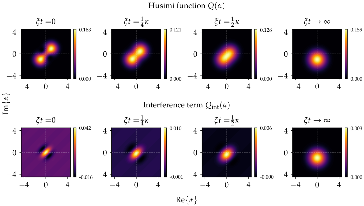
However, it is important to emphasize that the persistence of the interference term in Equation (33) does not imply the preservation of quantum coherence. As the system evolves, the dependence of the Husimi function on the initial coherent amplitudes is progressively erased, and the long-time dynamics becomes identical to that obtained from a single coherent-state initial condition. Figure 2 provides a direct visualization of the behavior described by Equation (29) for an initially even Schrödinger cat state | ψ ( 0 ) = C N | Γ 1 + | Γ 1 with Γ 1 = Γ 2 = 1 + i . The upper row shows the evolution of the complete Husimi function, where the two coherent components, Q 1 and Q 2 , progressively approach each other and eventually merge into a single stationary distribution. The lower row displays the corresponding interference contribution, Q int , making explicit the gradual transformation of the interference structure.

3.3. Fokker–Planck Equation

Since we already know how the Husimi function evolves in time, it is natural to expect that it satisfies a corresponding Fokker–Planck equation. This equation can be derived starting from the Lindblad master equation in the interaction picture, Equation (3), by taking its expectation value in coherent states, i.e., by projecting onto the coherent state basis as follows:
Tr { | α α | d ρ ^ d t } = Tr { | α α | i ξ a ^ + a ^ , ρ ^ + γ ( n th + 1 ) L [ a ^ ] ρ ^ + γ n th L [ a ^ ] ρ ^ } ,
where Tr { | α α | ρ ^ } = α | ρ ^ | α = π Q ( α ) . Taking into account the relation | α α | a ^ = α + α * | α α | [22], we obtain the corresponding Fokker–Planck equation
Q ( α , t ) t = i ξ α * α + γ α α + α * α * + 2 γ ( n th + 1 ) 2 α * α Q ( α , t ) .
The above equation is consistent with the usual phase-space Fokker–Planck treatments of driven–dissipative linear systems. In this form, the explicit distinction between drift and diffusion coefficients makes it evident that the Gaussian character of the channel is maintained, in line with the canonical structure of Gaussian quantum channels. The first contribution, proportional to ξ , accounts for the coherent driving of the field and results in a displacement of the phase-space distribution. The second contribution, proportional to γ , captures the dissipative evolution and produces a drift toward the steady state. The final contribution, proportional to γ ( n th + 1 ) , encodes the diffusion generated by the thermal environment, which leads to a broadening of the Husimi function.

4. Photon Statistics

The fact that an initially coherent state remains Gaussian throughout the evolution, as shown in Equation (21), greatly simplifies its characterization and enables a straightforward evaluation of relevant physical quantities, such as photon statistics, directly from the Husimi function through Equation (25) without the need to manipulate the density operator since these quantities depend only on first- and second-order moments. Having discussed interference effects for superpositions of coherent states in the previous subsection, we now return to the coherent state initial condition and analyze the statistical properties of the field. In particular, we calculate the temporal evolution of the photon number, the photon number standard deviation, and the Mandel parameter to investigate the effects of driving and dissipation on the system.

4.1. Mean Photon Number

Using Equation (25), the expectation value of the photon number operator is obtained as
n ^ ( t ) = a ^ a ^ 1 = Q ( α , t ) | α | 2 d 2 α 1 .
By performing the calculations using the Husimi function in Equation (21), which corresponds to the evolution of an initial coherent state, we obtain the expectation value of the photon-number operator in terms of the physical parameters.
n ^ ( t ) = n th + ξ 2 γ 2 2 ξ γ ξ γ + Γ y e γ t + Γ + i ξ γ 2 n th e 2 γ t .
The first term, n th , accounts for the thermal contribution of the reservoir. The second term, ξ 2 / γ 2 , corresponds to the steady-state excitation induced by the driving. The terms proportional to e γ t and e 2 γ t describe transient dynamics associated with the decay of the initial coherent state and its relaxation toward the stationary regime. We note that the mean photon number is time-independent when
Γ = ± n th i ξ γ .
In the long-time limit, the exponential terms vanish and the system reaches a stationary value given by
n ^ ss = n th + ξ 2 γ 2 ,
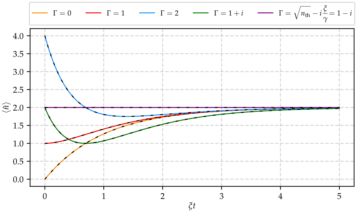
which clearly shows the combined contribution of thermal fluctuations and coherent driving. Figure 3 shows the time evolution of the average number of photons as a function of the scaled time ξ t for different initial coherent states of the system, including the case with time-independent mean photon number and for parameters κ = 1 and n th = 1 . The colored curves correspond to the analytical results given by Equation (37), while the dashed curves, in this and all subsequent figures, represent the numerical solutions obtained by solving the master Equation (3).
The numerical simulations were carried out using the QuTiP library in Python 3.13.7 [24], specifically employing the mesolve function. The Hilbert space of the field mode was truncated to a Fock basis with dimension N = 50 . Convergence was checked by increasing the cutoff to N = 51 ; for all the quantities plotted, the maximum absolute difference between both truncations was below 7 × 10 9 , which is negligible on the scale of the figures.

4.2. Photon-Number Standard Deviation

The fluctuations in the number of photons are characterized by the standard deviation,
Δ n ( t ) = n ^ 2 n ^ 2 ,
where n ^ 2 can be calculated using Equation (25) with the Husimi function obtained from an initial coherent state in Equation (21). After some algebra, we obtain
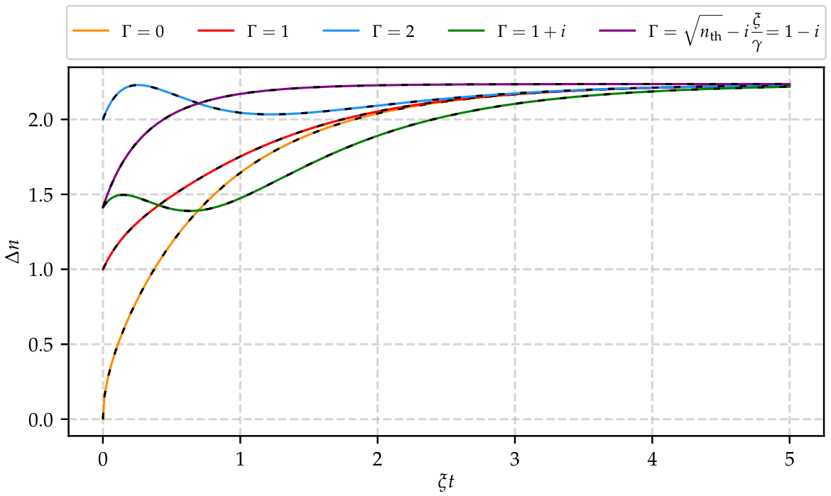
Δ n ( t ) = [ n th ( 1 + n th ) + ( 1 + 2 n th ) ξ 2 γ 2 2 ( 1 + 2 n th ) ξ γ ξ γ + Γ y e γ t + | Γ + i ξ γ | 2 n th ( 1 + 2 n th ) 2 n th ξ 2 γ 2 e 2 γ t + 4 n th ξ γ ξ γ + Γ y e 3 γ t + n th n th 2 | Γ + i ξ γ | 2 e 4 γ t ] 1 2 .
The standard deviation exhibits nontrivial transient dynamics characterized by multiple exponential decay rates, reflecting the interplay between the initial coherent state, coherent driving, dissipation, and thermal fluctuations. In the long-time limit, all transient contributions vanish, and the system approaches a stationary value given by
Δ n ss = n th ( 1 + n th ) + ( 1 + 2 n th ) ξ 2 γ 2 1 / 2 ,
which shows that the steady-state fluctuations arise from both thermal noise and coherent driving. This behavior is illustrated in Figure 4, where the time evolution of the standard deviation of the photon number is displayed for different initial coherent states.

4.3. Mandel Parameter

To further characterize the statistical properties of the field, we consider the Mandel parameter Q M , which provides a measure of the deviation of the photon statistics from a Poissonian distribution. It is defined in terms of the first and second moments of the photon-number operator as
Q M ( t ) = ( Δ n ^ ) 2 n ^ n ^ .
Negative values of Q M indicate sub-Poissonian statistics (nonclassical light), Q M = 0 corresponds to Poissonian statistics as in a coherent state, and Q M > 0 describes super-Poissonian behavior associated with enhanced fluctuations. Using the results obtained for the mean photon number and its variance, we find
Q M ( t ) = n th n ^ ( t ) 1 e 2 γ t n th ( 1 e 2 γ t ) + 2 ξ γ ξ γ + Γ y e γ t 2 + Γ x 2 e 2 γ t = n th 1 e 2 γ t 2 n th 1 e 2 γ t n ^ ( t ) .
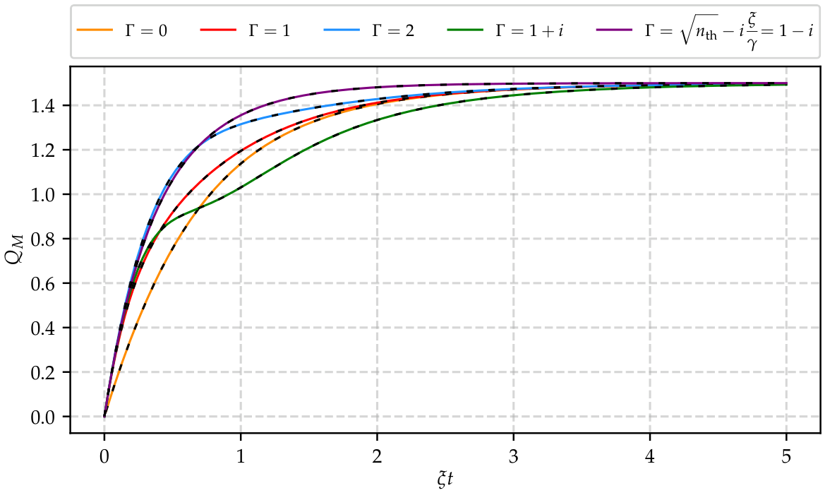
Several conclusions follow from the above expression. For the initial coherent state considered here, since n ^ 0 and ( 1 e 2 γ t ) 0 for t 0 , one has Q M ( t ) 0 at all times, indicating that the field remains restricted to Poissonian or super-Poissonian statistics during the evolution. In particular, for t = 0 , one obtains Q M ( 0 ) = 0 , as expected for an initial coherent state. Moreover, when n th = 0 , the Mandel parameter remains zero at all times, showing that, in the absence of thermal excitations, the field preserves Poissonian statistics. Therefore, the emergence of super-Poissonian behavior is entirely induced by the thermal reservoir. Figure 5 shows the time evolution of the Mandel parameter for different initial coherent amplitudes of the field. As expected for coherent states, all curves start from Q M = 0 , corresponding to Poissonian photon statistics. As time evolves, the interaction with the thermal reservoir induces super-Poissonian behavior, leading to positive values of Q M . Eventually, all trajectories converge toward the same stationary value.
We note that, in the steady state, the Mandel parameter is given by
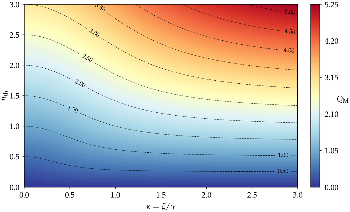
Q M s s = n th n th + 2 ξ γ 2 n th + ξ γ 2 .
Figure 6 illustrates the dependence of the steady-state Mandel parameter on the ratio κ = ξ / γ and on the average thermal occupation number n th .

5. Entropic Measures

Entropy measures provide complementary information about the evolution of the field state beyond photon statistics. Due to the Gaussian form of the state, the known Wehrl entropy [25], an entropy of a quantum state in terms of coherent states, can be directly evaluated from the Husimi function, reinforcing the usefulness of the phase-space approach adopted here. We also calculate the linear entropy, which quantifies the loss of purity caused by the interaction with the thermal reservoir.

5.1. Wehrl Entropy

The Wehrl entropy [25] is an entropy defined over the Husimi Q-function that captures phase-space uncertainties of a quantum state. Beyond its foundational role, it has proven useful in characterizing the degree of squeeze of squeezed states [26] and has been proposed as a measure of the nonclassicality of bosonic states [27,28]. It is defined as
S W ( ρ ^ ) = d 2 α Q ( α ) ln ( π Q ( α ) ) .
Substituting the result in Equation (21) into the definition above, we obtain a closed-form expression for the Wehrl entropy
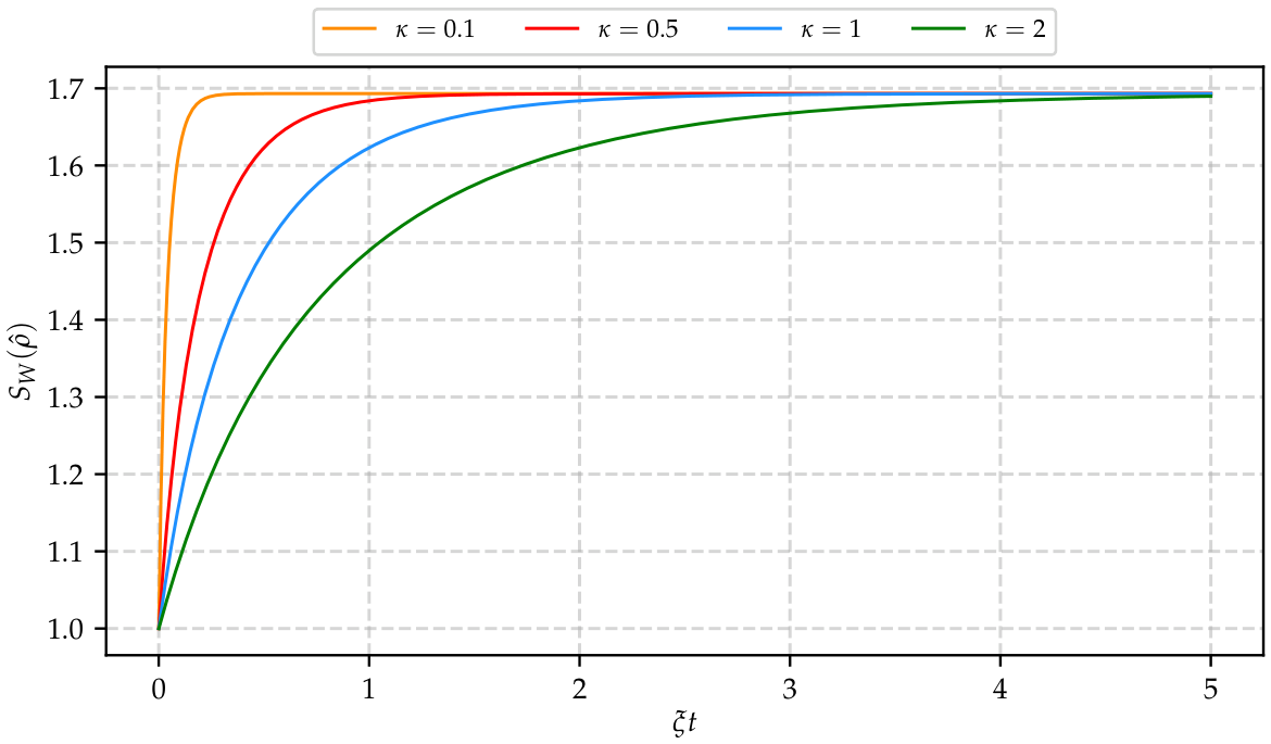
S W ( ρ ^ ) = 1 + ln 1 + n th ( 1 e 2 γ t ) .
Several physically meaningful conclusions can be drawn from this expression. First, at t = 0 , the Wehrl entropy reduces to S W = 1 , which is the known minimum value attained by a coherent state [29], consistent with the initial condition of the system. Second, in the zero-temperature limit ( n th = 0 ), the entropy remains equal to unity for all times, reflecting the fact that the reservoir does not introduce thermal fluctuations and the state retains its coherent character. Third, for n th > 0 , the entropy grows monotonically in time, quantifying the progressive increase in the phase-space uncertainty due to thermal decoherence. Finally, as t , the entropy saturates at the asymptotic value S W s s = 1 + ln ( 1 + n th ) , which depends solely on the reservoir temperature and corresponds to the thermal equilibrium state of the field independently of the driving strength ξ . Figure 7 shows the time evolution of the Wehrl entropy for different values of κ . It can be observed that increasing γ , that is, reducing κ , causes the entropy to approach its stationary value more rapidly.

5.2. Linear Entropy

As a complementary measure of mixedness that directly quantifies how driving and dissipation affect the purity of the evolved state, we compute the linear entropy, given by
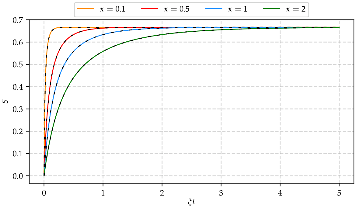
S = 1 Tr { ρ ^ 2 } = 1 θ 2 θ = 1 1 1 + 2 n th ( 1 e 2 γ t ) ,
where Tr { ρ ^ 2 } is the purity of the state. Unlike the Wehrl entropy, S L vanishes exactly for a pure state and approaches unity for a maximally mixed state, providing a more direct measure of the degree of mixing. Linear entropy displays a qualitatively similar behavior to S W : it grows monotonically from S L ( 0 ) = 0 , saturates at the asymptotic value S s s = 1 1 / ( 1 + 2 n th ) , and the approach to equilibrium is governed by the same timescale ( 2 γ ) 1 . This is illustrated in Figure 8, where the effect of increasing γ is again to accelerate thermalization.
It is important to note that the linear entropy is determined exclusively by the reservoir parameters, namely the damping rate γ and the mean thermal excitation number n th , and is independent of the driving force ξ . This follows from the fact that the classical driving induces only a unitary displacement in phase space, whereas purity, or the linear entropy, is invariant under unitary transformations. It is worth noting the particular case n th = 0 , which corresponds to a reservoir at zero temperature. In this limit, the linear entropy vanishes identically, S = 0 , at all times. This result has a clear physical interpretation: in the absence of thermal fluctuations, the only effect of the reservoir is to damp the field amplitude, while the classical driving continuously displaces the state in phase space. Since coherent states remain coherent under both amplitude damping at zero temperature and coherent displacement, the system preserves its purity throughout evolution regardless of the value of γ . Therefore, the loss of purity originates entirely from thermal fluctuations in the reservoir.

6. Conclusions

We have presented a comprehensive analytical treatment of a driven quantum field coupled to a finite-temperature reservoir using a phase-space approach based on the Husimi Q-function. Starting from the Lindblad master equation, by applying a rotating-frame transformation followed by a displacement operation, the explicit time dependence introduced by the coherent driving was eliminated, reducing the problem to the well-known master equation for a lossy cavity field at finite temperature, solvable via superoperator techniques.
A central result is the derivation of a closed Gaussian form for the Husimi function of an initially coherent state. The Gaussian structure is preserved throughout the evolution, whereas the stationary state corresponds to a displaced thermal state. This representation shows that coherent driving determines the trajectory of the phase-space distribution through a displacement of its center, while the thermal reservoir controls its broadening and stationary width. In particular, for a zero-temperature reservoir, the Gaussian width remains unchanged, indicating that an initial coherent state preserves its purity during evolution. Furthermore, the Husimi representation enables an analytical description of the superposition of coherent states, showing that the driving field determines the position of the interference structure in phase space, whereas dissipation and thermal fluctuations progressively erase the signatures of the initial superposition. Consequently, the long-time dynamics becomes independent of the initial coherent amplitudes and converges to a unique stationary displaced thermal state. Furthermore, we derive the corresponding Fokker–Planck equation, which confirms that the Husimi function encodes the complete dynamics of the system while identifying the roles of coherent driving, dissipation, and thermal fluctuations in shaping the phase-space distribution.
All the relevant photon statistics were obtained in closed form: the mean photon number and standard deviation converge to stationary values reflecting the combined effect of thermal excitations and driving, while the Mandel parameter remains non-negative at all times, confirming that sub-Poissonian statistics are entirely absent and that super-Poissonian behavior is exclusively induced by the thermal reservoir.
The entropic analysis revealed that both the Wehrl and linear entropies grow monotonically from their initial values and saturate at equilibrium values determined solely by the reservoir temperature independently of the driving strength. This independence reflects the unitary nature of coherent displacement, which cannot alter the purity of the state. In the zero-temperature limit, purity is preserved throughout the entire evolution. It is important to emphasize that the present analysis is limited to a Markovian Lindblad description with constant damping and thermal rates. This assumption enables the superoperator solution and the closed Husimi representation, but it excludes reservoir-memory effects. In related non-Markovian cavity models [30,31], such effects are incorporated through an explicit system–reservoir coupling, which gives rise to time-dependent coefficients in the reduced master equation and allows the Markovian limit to be recovered by increasing the environmental spectral width. These effects could modify the transient phase-space distribution, photon statistics, and entropy measures. Thus, our results provide an analytical characterization of the driven–dissipative field within the Markovian regime.
From an experimental perspective, the theoretical framework developed here can be realized in state-of-the-art quantum optical platforms. In cavity QED and circuit QED architectures, the coupling of a quantized field mode to a classical drive and a thermal bath with well-controlled parameters has been widely demonstrated. Realistic values of the dissipation rate γ and the resonant driving force ξ can be adjusted over a wide range, while the thermal excitation number n th can be tuned by controlling the cryogenic temperature of the environment or by injecting artificial thermal noise. The predicted stationary displaced thermal state and the super-Poissonian photon statistics can be measured using standard reconstruction techniques. For instance, the Husimi Q-function can be directly probed via tomographic methods or heterodyne detection, while the Mandel parameter and photon-number fluctuations can be characterized through photon-number-resolving detectors or correlation measurements of the output field in superconducting circuits [32]. Similar phase-space descriptions under related environmental conditions have been discussed in [19].
In summary, the Husimi-function approach provides an elegant and analytically tractable framework for characterizing driven–dissipative quantum fields, yielding closed-form expressions for all relevant quantities without requiring explicit manipulation of the density operator. The results obtained constitute a self-consistent and complete characterization of the field’s phase-space, statistical, and entropic properties and generalize previous studies of lossy cavity fields by explicitly incorporating the effect of a resonant classical driving term.

Author Contributions

Conceptualization, M.A.G.-M. and H.M.M.-C.; methodology, M.A.G.-M., I.R.-P., F.S.-E. and H.M.M.-C.; investigation, M.A.G.-M. and H.M.M.-C.; writing—original draft, M.A.G.-M., I.R.-P., F.S.-E. and H.M.M.-C.; supervision, H.M.M.-C. All authors have read and agreed to the published version of the manuscript.

Funding

This research received no external funding.

Data Availability Statement

No new data were created or analyzed in this study. Data sharing is not applicable to this article.

Acknowledgments

Marco Antonio García-Márquez thanks the Secretariat of Science, Humanities, Technology and Innovation (SECIHTI) and the National Institute of Astrophysics, Optics and Electronics (INAOE) for the doctoral scholarship.

Conflicts of Interest

The authors declare no conflicts of interest.

Appendix A. Derivation of the Husimi Function for an Initial Coherent-State Superposition

Considering the initial condition given in Equation (28), we obtain the corresponding density operator
ρ ^ ( 0 ) = | C N | 2 | Γ 1 Γ 1 | + | Γ 2 Γ 2 | + | Γ 1 Γ 2 | + | Γ 2 Γ 1 | ,
where the last two terms correspond to the interference contributions. For an arbitrary initial condition, the Husimi function is given by
Q ( α , t ) = 1 π α | D ^ ( η ) e 2 β t + f 3 ( t ) e f 2 ( t ) J ^ 2 e f 0 ( t ) L ^ e f 1 ( t ) J ^ 1 D ^ ( η ) ρ ^ ( 0 ) D ^ ( η ) D ^ ( η ) | α .
Therefore, it is sufficient to determine the evolution of a general operator of the form | Γ m Γ n | . First, we use the relation
D ^ ( η ) | Γ m Γ n | D ^ ( η ) = e i Im { η ( Γ m * Γ n * ) } | Γ m η Γ n η | .
Furthermore, the action of the superoperators can be successively evaluated as
e f 1 J ^ 1 | Γ m η Γ n η | = k = 0 f 1 k k ! J ^ 1 k | Γ m η Γ n η | = e 2 f 1 ( Γ m η ) ( Γ n η ) * | Γ m η Γ n η | ,
e f 0 L ^ | Γ m η Γ n η | = e f 0 n ^ | Γ m η Γ n η | e f 0 n ^ = e 1 2 ( 1 e 2 f 0 ) ( | Γ m η | 2 + | Γ n η | 2 ) | ( Γ m η ) e f 0 ( Γ n η ) e f 0 | ,
e f 2 J ^ 2 | ( Γ m η ) e f 0 ( Γ n η ) e f 0 | = k = 0 f 2 k k ! J ^ 2 k | ( Γ m η ) e f 0 ( Γ n η ) e f 0 | = k = 0 ( 2 f 2 ) k k ! a ^ k | ( Γ m η ) e f 0 ( Γ n η ) e f 0 | a ^ k .
Therefore, the evolution of a general operator | Γ m Γ n | is given by
1 π α | D ^ ( η ) e 2 β t + f 3 ( t ) e f 2 ( t ) J ^ 2 e f 0 ( t ) L ^ e f 1 ( t ) J ^ 1 D ^ ( η ) | Γ m Γ n | D ^ ( η ) D ^ ( η ) | α = 1 π e i Im { η ( Γ m * Γ n * ) } e 2 β t + f 3 e 1 2 ( 1 e 2 f 0 ) ( | Γ m η | 2 + | Γ n η | 2 ) e 2 f 1 ( Γ m η ) ( Γ n η ) * × k = 0 ( 2 f 2 ) k k ! α η | a ^ k | ( Γ m η ) e f 0 ( Γ n η ) e f 0 | a ^ k | α η = 1 π e i Im { η ( Γ m * Γ n * ) } e 2 β t + f 3 e 1 2 ( | Γ m η | 2 + | Γ n η | 2 ) e 2 f 1 ( Γ m η ) ( Γ n η ) * × e | α η | 2 ( 1 2 f 2 ) e ( ( α η ) * ( Γ m η ) + ( α η ) ( Γ n η ) * ) e f 0 ,
where the summation has been simplified according to
k = 0 ( 2 f 2 ) k k ! α η | a ^ k | ( Γ m η ) e f 0 ( Γ n η ) e f 0 | a ^ k | α η = e 2 f 2 | α η | 2 α η | ( Γ m η ) e f 0 ( Γ n η ) e f 0 | α η = e | α η | 2 ( 1 2 f 2 ) e 1 2 e 2 f 0 ( | Γ m η | 2 + | Γ n η | 2 ) e ( ( α η ) * ( Γ m η ) + ( α η ) ( Γ n η ) * ) e f 0 .
By applying Equation (A6) to each term in Equation (A1), the complete Husimi function can be written as
Q ( α , t ) = | C N | 2 π e 2 β t + f 3 e | α η | 2 ( 1 2 f 2 ) j = 1 , 2 e | Γ j η | 2 ( 1 2 f 1 ) e 2 e f 0 Re { ( α η ) ( Γ j * η * ) } + 2 | C N | 2 π e 2 β t + f 3 e 1 2 ( | Γ 1 η | 2 + | Γ 2 η | 2 ) e | α η | 2 ( 1 2 f 2 ) × Re e i Im { η ( Γ 1 * Γ 2 * ) } e 2 f 1 ( Γ 1 η ) ( Γ 2 η ) * e ( ( α η ) * ( Γ 1 η ) + ( α η ) ( Γ 2 η ) * ) e f 0 .
where the first two contributions describe the evolution of the diagonal coherent-state components, | Γ j Γ j | , with j = 1 , 2 , whereas the last term corresponds to the evolution of the off-diagonal coherent-state components, | Γ 1 Γ 2 | and | Γ 2 Γ 1 | . Finally, by substituting the explicit expressions for the functions f i ( t ) and simplifying the resulting expression, Equation (29) is obtained.

References

  1. Walls, D.F.; Milburn, G.J. Effect of dissipation on quantum coherence. Phys. Rev. A 1985, 31, 2403–2408. [Google Scholar] [CrossRef] [Scilit] [PubMed]
  2. Milburn, G.J.; Walls, D.F. Effect of dissipation on interference in phase space. Phys. Rev. A 1988, 38, 1087–1090. [Google Scholar] [CrossRef] [Scilit] [PubMed]
  3. Louisell, W.H.; Walker, L.R. Density-Operator Theory of Harmonic Oscillator Relaxation. Phys. Rev. 1965, 137, B204–B211. [Google Scholar] [CrossRef] [Scilit]
  4. Carusotto, S. Relaxation of a driven harmonic oscillator. Phys. Rev. A 1975, 11, 1407–1413. [Google Scholar] [CrossRef] [Scilit]
  5. Bang-Pin, H.; Shun-Jin, W.; Wan-Lun, Y. An Exact Solution to the Master Equation for the Dissipative Harmonic Oscillator Driven by an External Field. Chin. Phys. Lett. 2003, 20, 979–981. [Google Scholar] [CrossRef] [Scilit]
  6. Moussa, M.; Mizrahi, S.; Caldeira, A. Quantum coherence in a dissipative-driven system and the optical Stern-Gerlach experiment. Phys. Lett. A 1996, 221, 145–152. [Google Scholar] [CrossRef] [Scilit]
  7. Carmichael, H. An Open Systems Approach to Quantum Optics. In Lecture Notes in Physics Monographs, 1st ed.; Springer: Berlin/Heidelberg, Germany, 1993; Volume 18. [Google Scholar] [CrossRef] [Scilit]
  8. Mufti, A.; Schmitt, H.A.; Balantekin, A.B.; Sargent, M. Analytical solution to the master equation for a quantized cavity mode. J. Opt. Soc. Am. B 1993, 10, 2100–2106. [Google Scholar] [CrossRef] [Scilit]
  9. Arnoldus, H.F. Density matrix for photons in a cavity. J. Opt. Soc. Am. B 1996, 13, 1099–1106. [Google Scholar] [CrossRef] [Scilit]
  10. Castro Neto, A.H.; Caldeira, A.O. Quantum dynamics of an electromagnetic mode in a cavity. Phys. Rev. A 1990, 42, 6884–6893. [Google Scholar] [CrossRef] [Scilit] [PubMed]
  11. Hernández-Sánchez, L.; Ramos-Prieto, I.; Soto-Eguibar, F.; Moya-Cessa, H.M. Exact solution for the interaction of two decaying quantized fields. Opt. Lett. 2023, 48, 5435–5438. [Google Scholar] [CrossRef] [Scilit] [PubMed]
  12. Hernández-Sánchez, L.; Bocanegra-Garay, I.A.; Ramos-Prieto, I.; Soto-Eguibar, F.; Moya-Cessa, H.M. Effective non-Hermitian formulation of the Lindblad equation for interacting quantized fields at finite temperature. Phys. Rev. A 2025, 112, L021702. [Google Scholar] [CrossRef] [Scilit]
  13. Hernández-Sánchez, L.; Ramos-Prieto, I.; Soto-Eguibar, F.; Moya-Cessa, H.M. Dynamics of the Interaction Between Two Coherent States in a Cavity with Finite Temperature Decay. Dynamics 2025, 5, 4. [Google Scholar] [CrossRef] [Scilit]
  14. Arévalo-Aguilar, L.M.; Moya-Cessa, H. Solution to the master equation for a quantized cavity mode. Quantum Semiclassical Opt. J. Eur. Opt. Soc. Part B 1998, 10, 671–674. [Google Scholar] [CrossRef] [Scilit]
  15. Jie, Y.; Huai-Xin, L.; Bo, Z.; Mei-Sheng, Z.; Yong-De, Z. Solution to the Master Equation of a Free Damped Harmonic Oscillator with Linear Driving. Chin. Phys. Lett. 2003, 20, 796–798. [Google Scholar] [CrossRef] [Scilit]
  16. Meng, X.G.; Wang, J.S.; Gao, H.C. Kraus Operator-Sum Solution to the Master Equation Describing the Single-Mode Cavity Driven by an Oscillating External Field in the Heat Reservoir. Int. J. Theor. Phys. 2016, 55, 3630–3636. [Google Scholar] [CrossRef] [Scilit]
  17. Saito, H.; Hyuga, H. Relaxation of Schrödinger Cat States and Displaced Thermal States in a Density Operator Representation. J. Phys. Soc. Jpn. 1996, 65, 1648–1654. [Google Scholar] [CrossRef] [Scilit]
  18. Mattos, E.; Vidiella-Barranco, A. Time evolution of the quantized field coupled to a thermal bath: A phase space approach. Ann. Phys. 2020, 422, 168321. [Google Scholar] [CrossRef] [Scilit]
  19. Mattos, E.; Vidiella-Barranco, A. Phase-space approach to cavity field dynamics in a squeezed thermal reservoir. Ann. Phys. 2025, 479, 170055. [Google Scholar] [CrossRef] [Scilit]
  20. Walls, D.F.; Milburn, G.J. Quantum Optics, 2nd ed.; Springer: Berlin/Heidelberg, Germany, 2008. [Google Scholar] [CrossRef] [Scilit]
  21. Glauber, R.J. Coherent and Incoherent States of the Radiation Field. Phys. Rev. 1963, 131, 2766–2788. [Google Scholar] [CrossRef] [Scilit]
  22. Louisell, W.H. Quantum Statistical Properties of Radiation; John Wiley & Sons: New York, NY, USA, 1990. [Google Scholar]
  23. Scully, M.O.; Zubairy, M.S. Quantum Optics; Cambridge University Press: Cambridge, UK, 1997. [Google Scholar]
  24. Johansson, J.; Nation, P.; Nori, F. QuTiP 2: A Python framework for the dynamics of open quantum systems. Comput. Phys. Commun. 2013, 184, 1234–1240. [Google Scholar] [CrossRef] [Scilit]
  25. Wehrl, A. On the relation between classical and quantum-mechanical entropy. Rep. Math. Phys. 1979, 16, 353–358. [Google Scholar] [CrossRef] [Scilit]
  26. Lee, C. Wehrl’s entropy as a measure of squeezing. Opt. Commun. 1988, 66, 52–54. [Google Scholar] [CrossRef] [Scilit]
  27. Bose, S. Wehrl-entropy-based quantification of nonclassicality for single-mode quantum optical states. J. Phys. A Math. Theor. 2018, 52, 025303. [Google Scholar] [CrossRef] [Scilit]
  28. Zhang, Y.; Luo, S. Entropy excesses as quantifiers of nonclassicality. Eur. Phys. J. Plus 2021, 136, 464. [Google Scholar] [CrossRef] [Scilit]
  29. Lieb, E.H. Proof of an entropy conjecture of Wehrl. Commun. Math. Phys. 1978, 62, 35–41. [Google Scholar] [CrossRef] [Scilit]
  30. Shen, H.Z.; Shang, C.; Zhou, Y.H.; Yi, X.X. Unconventional single-photon blockade in non-Markovian systems. Phys. Rev. A 2018, 98, 023856. [Google Scholar] [CrossRef] [Scilit]
  31. Shen, H.Z.; Wang, Q.; Wang, J.; Yi, X.X. Nonreciprocal unconventional photon blockade in a driven dissipative cavity with parametric amplification. Phys. Rev. A 2020, 101, 013826. [Google Scholar] [CrossRef] [Scilit]
  32. Schuster, D.I.; Houck, A.A.; Schreier, J.A.; Wallraff, A.; Gambetta, J.M.; Blais, A.; Frunzio, L.; Majer, J.; Johnson, B.; Devoret, M.H.; et al. Resolving photon number states in a superconducting circuit. Nature 2007, 445, 515–518. [Google Scholar] [CrossRef] [Scilit] [PubMed]
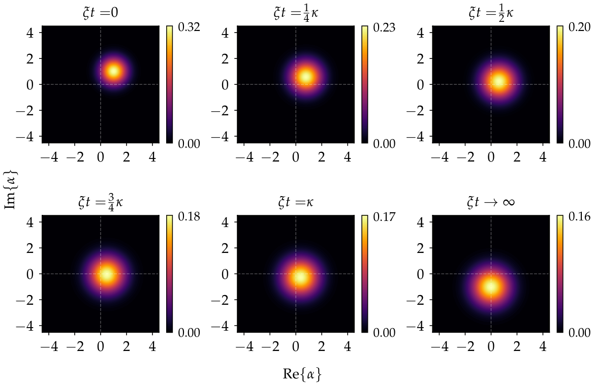
Figure 1. Time evolution of the Husimi function for different values of the scaled time ξ t , showing the phase-space displacement due to the driving and the broadening induced by dissipation and thermal fluctuations. The initial state is a coherent state | Γ with Γ = 1 + i . Results are shown for κ = 1 and n th = 1 .
Dynamics 06 00026 g001
Figure 2. Time evolution of the Husimi function and its interference contribution for an initial even Schrödinger cat state, | ψ ( 0 ) = C N | Γ 1 + | Γ 1 , with Γ 1 = 1 + i . The upper row shows the Husimi function, while the lower row displays the corresponding interference contribution given by the third term in Equation (29). The panels correspond to different values of the scaled time ξ t , illustrating the progressive merging of the coherent components and the evolution of the interference contribution toward its stationary form. Results are shown for κ = 1 and n th = 1 .
Dynamics 06 00026 g002
Figure 3. Average number of photons as a function of the scaled time ξ t for different initial coherent states, with parameters κ = 1 and n th = 1 , showing convergence toward a unique stationary value independent of the initial condition.
Dynamics 06 00026 g003
Figure 4. Standard deviation of the photon number as a function of the scaled time ξ t for different initial coherent states, with κ = 1 and n th = 1 .
Dynamics 06 00026 g004
Figure 5. Mandel parameter Q M as a function of the scaled time ξ t for different initial coherent amplitudes of the field, with parameters κ = 1 and n th = 1 .
Dynamics 06 00026 g005
Figure 6. Steady-state Mandel parameter Q M as a function of κ and n th .
Dynamics 06 00026 g006
Figure 7. Wehrl entropy S W as a function of the scaled time ξ t for different values of κ and a fixed mean thermal excitation number n th = 1 .
Dynamics 06 00026 g007
Figure 8. Linear entropy as a function of the scaled time ξ t for different values of the parameter κ and with n th = 1 .
Dynamics 06 00026 g008
Disclaimer/Publisher’s Note: The statements, opinions and data contained in all publications are solely those of the individual author(s) and contributor(s) and not of MDPI and/or the editor(s). MDPI and/or the editor(s) disclaim responsibility for any injury to people or property resulting from any ideas, methods, instructions or products referred to in the content.