Temporal Ramsey Graphs: The Ramsey Kinematic Approach to the Motion of Systems of Material Points

Abstract

The Ramsey approach is applied to analyses of the kinematics of systems built of non-relativistic, motile point masses/particles. This approach is based on colored graph theory. Point masses/particles serve as the vertices of the graph. The time dependence of the distance between the particles determines the coloring of the links. The vertices/particles are connected with orange links when particles move away from each other or remain at the same distance. The vertices/particles are linked with violet edges when particles converge. The sign of the time derivative of the distance between the particles dictates the color of the edge. Thus, a complete, bi-colored Ramsey temporal graph emerges. The suggested coloring procedure is not transitive. The coloring of the links is time-dependent. The proposed coloring procedure is frame-independent and insensitive to Galilean transformations. At least one monochromatic triangle will inevitably appear in the graph emerging from the motion of six particles due to the fact that the Ramsey number $R\left(\mathrm{3,3}\right)=6.$ This approach is extended to the analysis of systems containing an infinite number of moving point masses. An infinite monochromatic (violet or orange) clique will necessarily appear in the graph. Applications of the introduced approach are discussed. The suggested Ramsey approach may be useful for the analysis of turbulence seen within the Lagrangian paradigm.

1. Introduction

The synthesis of novel fields of mathematics and physics is extremely fruitful and sometimes generates and even constitutes new fields of investigation [1,2,3]. Nobel Prize winner Eugene Paul Wigner, in his seminal paper, even spoke about the “unreasonable effectiveness of mathematics in the natural sciences” [1]. One of the most advanced fields of modern mathematics is graph theory, which has been developed extensively in recent decades [4,5]. A mathematical graph is a structure used to represent the relationships between objects. Simply speaking, graphs represent a set of objects and a set of pairwise relations between them [4,5]. They consist of vertices/nodes, which are the fundamental units or points in the graph, and edges/links, which are the connections between the vertices [4,5,6]. One variety of graph is the so-called colored graph, which is a graph in which colors are assigned to its elements, typically its vertices or edges [6,7,8]. The classical result in the theory of colored graphs (which is referred to as the Ramsey theorem) states that for any given integers r and s, a minimum number exists $\mathit{R}\left(\mathit{r},\mathit{s}\right)$, called the Ramsey number, such that any graph on at least $\mathit{R}\left(\mathit{r},\mathit{s}\right)$ vertices, with the edges colored in two colors (say, orange and violet), will contain either an orange clique of size r (i.e., a complete subgraph ${\mathit{K}}_{\mathit{r}}$ where all of the edges are orange) or a violet clique of size s (i.e., a complete subgraph ${\mathit{K}}_{\mathit{s}}$ where all of the edges are violet) [8,9,10,11,12,13,14,15]. Graph theory demonstrates potential for physics; however, to date, applications of graph theory to physics have been scarce [16,17,18,19,20,21,22]. We introduce a graph scheme applicable to analyses of the motion of systems of material points which results in a temporal, complete, bi-colored graph [23,24,25]. We extend our approach to infinite systems built of material points.

2. Results

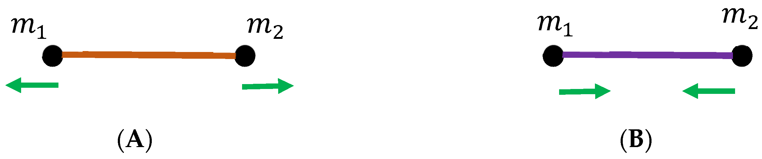
2.1. A Coloring Procedure Applicable to the Motion of Point Masses: Bi-Coloring for a Pair of Particles

Let us introduce the coloring procedure, which is applicable to the motion of N point masses $m_i,i=1,\dots ,N.$ The procedure will eventually give rise to a complete, bi-colored, temporal graph. Consider first the simplest system built of two non-relativistic moving point masses/particles $m_1$ and $m_2$, depicted in Figure 1.

The Cartesian coordinates of the point masses $m_1$ and $m_2$ are $\left(x_{11}\left(t\right),x_{12}\left(t\right),x_{13}\left(t\right)\right)$ and $\left(x_{21}\left(t\right),x_{22}\left(t\right),x_{23}\left(t\right)\right)$, respectively; the first index denotes the number of the particle, and the second index denotes the number of the Cartesian coordinates (see Figure 1). The time-dependent distance between the point masses $r_{12}\left(t\right)$ is given using Equation (1):

$$r_{12}\left(t\right)=\sqrt{{\left(x_{21}\left(t\right)-x_{11}(t\right)}^2+{\left(x_{22}\left(t\right)-x_{12}\left(t\right)\right)}^2+{\left(x_{23}\left(t\right)-x_{13}\left(t\right)\right)}^2}$$

(1)

Now, we introduce the following coloring procedure: from a purely kinematic point of view, two situations are possible: (i) the particles become closer/(converge) in the course of their motion, or (ii) they move away from each other/remain at the same distance. When the particles move away from each other or remain at the same distance, Equation (2) applies:

$${\displaystyle \frac{d\left(r_{12}\left(t\right)\right)}{dt}}\ge 0$$

(2)

When the particles converge, Equation (3) holds true:

$${\displaystyle \frac{d\left(r_{12}\left(t\right)\right)}{dt}}<0$$

(3)

Now, we take an instant photograph of the pair of particles$m_1$ and $m_2$ at $t=t_0$.

We adopt the following coloring procedure: if the particles $m_1$ and $m_2$ move away from each other or remain at the same distance and Equation (2) applies, they are connected with an orange link (they are “strangers” in the terms of the seminal “party problem” of Ramsey theory [10,11,12,13]), and when the particles converge and Equation (3) holds true, they are connected with a violet link (they are considered, respectively, “friends” [10,11,12,13]), as shown in Figure 2.

Consider that the coloring presented in Figure 2 holds when particles $m_1$ and $m_2$ are at rest relative to each other. The introduced coloring is time-dependent. It is noteworthy that Equations (2) and (3) exhaust all of the possibilities of relative motion for the given pair of particles. It also should be emphasized that the introduced coloring is completely based on the kinematic considerations, and it neglects the dynamic details of the interaction between the point masses. The coloring scheme is trivially extended to any generalized coordinates of the particles (cylindrical, spherical, etc.). The introduced coloring scheme is frame-independent; consider that the particles are non-relativistic. Thus, the distance between the particles is invariant in all of the frames, both inertial and non-inertial.

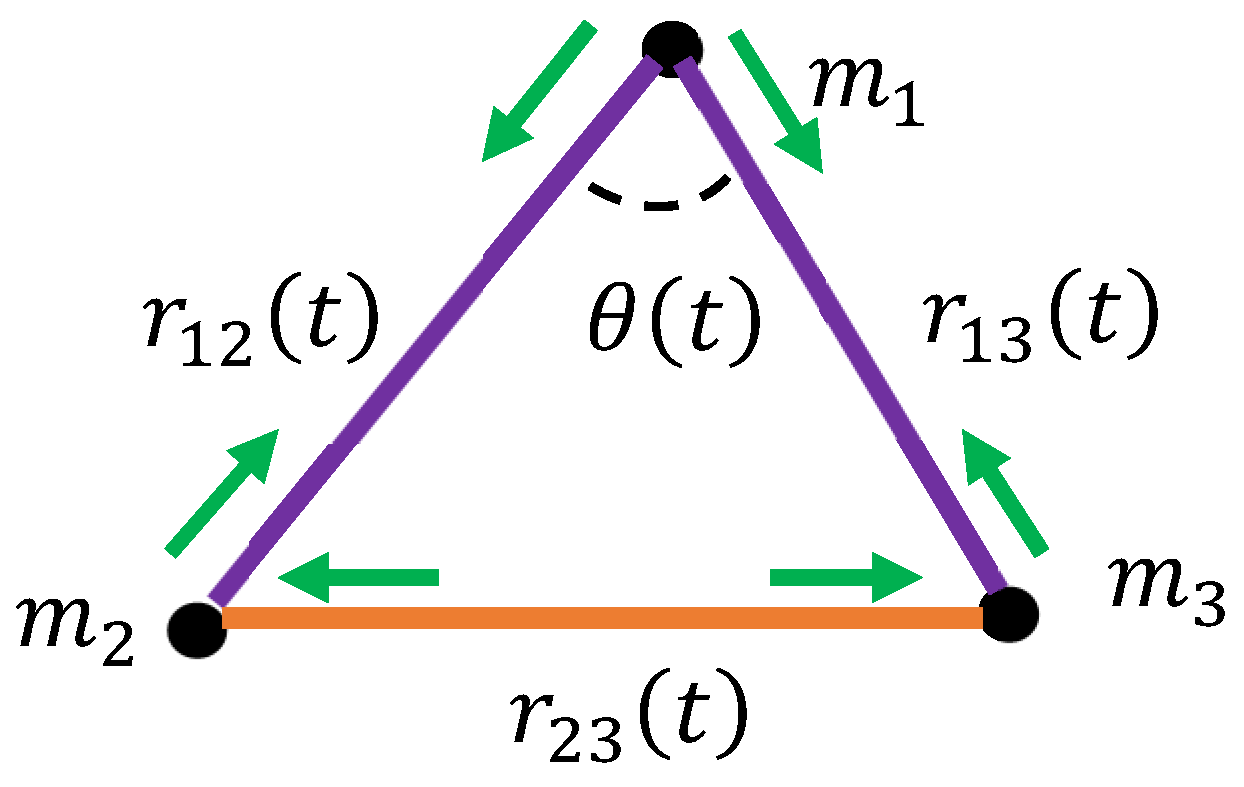
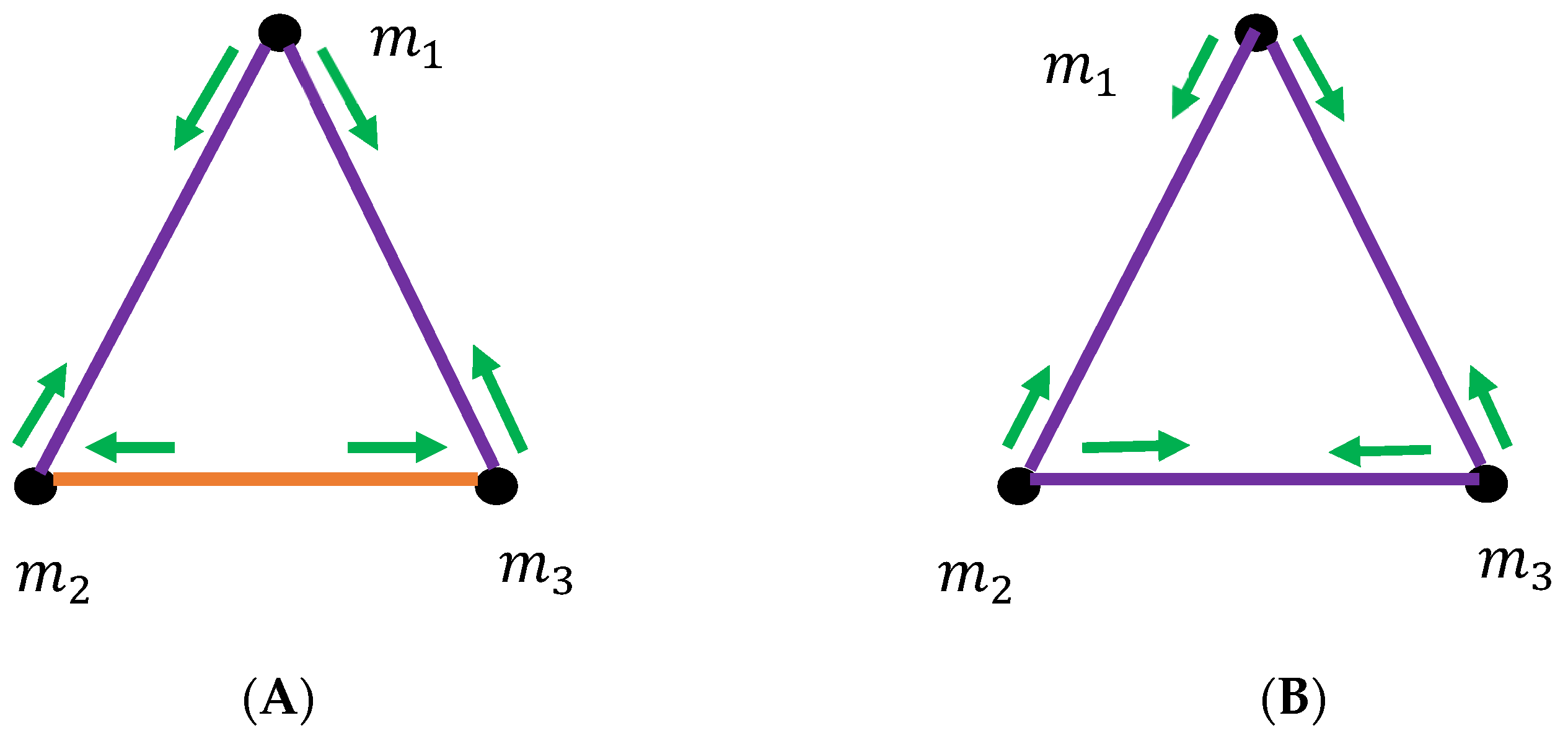
2.2. The Coloring for a Triad of Particles: Checking the Transitivity of the Coloring Procedure

Now, we apply the introduced procedure to the triad of moving particles $m_1,m_2,$ and $m_3$. These particles serve as the vertices of the graph. The coloring procedure is supplied by Equations (2) and (3). It seems from first glance that the application of the introduced coloring scheme is straightforward for the triad of particles. However, the situation is much more subtle, and the transitivity of the coloring should be carefully examined [26,27,28]. Actually, the internal logic of the graph influences its coloring [26,27,28]. Let us illustrate this with the scheme depicted in Figure 3. Consider the triad of moving particles $m_1,m_2,$ and $m_3$ shown in Figure 3. Assume that particles $m_1$and $m_2$ converge, i.e., ${\displaystyle \frac{d\left(r_{12}\left(t\right)\right)}{dt}}<0$ holds. We also assume that particles $m_1$and $m_3$ converge, i.e., ${\displaystyle \frac{d\left(r_{13}\left(t\right)\right)}{dt}}<0$. Does this necessarily mean that particles $m_2$and $m_3$ also necessarily converge? If this is true, the suggested coloring procedure is transitive. In other words, the transitivity means that if the pairs of particles $m_2$ and $m_1$ and $m_1$ and $m_3$ are connected with a violet link, this necessarily implies that particles $m_2$ and $m_3$are also connected with a violet link. This is not true, as will be demonstrated below.

The transitivity of the coloring has crucial importance for the analysis of the emerging graph. It has been demonstrated that the transitive Ramsey numbers are different from those calculated for non-transitive graphs [26,27,28]. This is quite understandable; indeed, if the coloring is transitive, a monochromatic triangle immediately emerges for any pair of mono-colored, adjacent edges. It is easy to demonstrate that the introduced coloring is not transitive. The distance between particles $m_2$ and $m_3$ is given by

$$r_{23}^2\left(t\right)=r_{12}^2\left(t\right)+r_{13}^2\left(t\right)-2r_{12}\left(t\right)r_{13}\left(t\right)cos\theta \left(t\right),$$

(4)

where $r_{12}\left(t\right),r_{13}\left(t\right),r_{23}\left(t\right),\mathrm{a}\mathrm{n}\mathrm{d}\theta \left(t\right)$are shown in Figure 3. Consider a situation where $r_{12}\left(t\right)\mathrm{a}\mathrm{n}\mathrm{d}{r}_{13}\left(t\right)$ are slowly changing, decreasing functions, whereas $\theta \left(t\right)<{\displaystyle \frac{\pi }{2}}$ is a rapidly growing function. These assumptions may be quantified within a linear approximation: consider the motion in which $r_{12}\left(t\right)=r_{13}\left(t\right)=r_0-\alpha t,\theta =\omega t;\alpha =const;\omega =const.$ Routine calculations demonstrate that when $\omega t\cong {\displaystyle \frac{\pi }{2}}$ and $\left(r_0-\alpha t\right)\omega \gg 2\alpha$, ${\displaystyle \frac{d\left(r_{23}\left(t\right)\right)}{dt}}>0$ is true. Thus, it is possible that the $r_{23}\left(t\right)$ link is orange when $r_{12}\left(t\right)\mathrm{a}\mathrm{n}\mathrm{d}{r}_{13}\left(t\right)\mathrm{a}\mathrm{r}\mathrm{e}\mathrm{v}\mathrm{i}\mathrm{o}\mathrm{l}\mathrm{e}\mathrm{t},$and both of the situations depicted in Figure 4 are possible. When $r_{12}\left(t\right)\mathrm{a}\mathrm{n}\mathrm{d}{r}_{13}\left(t\right)$ are constant, the coloring is obviously non-transitive: $\theta \left(t\right)$ may grow or decrease with time.

Similar reasoning leads to the conclusion that the orange coloring is also non-transitive. We conclude that the suggested colored procedure defined by Equations (2) and (3) is not transitive. And, again, it is frame-independent.

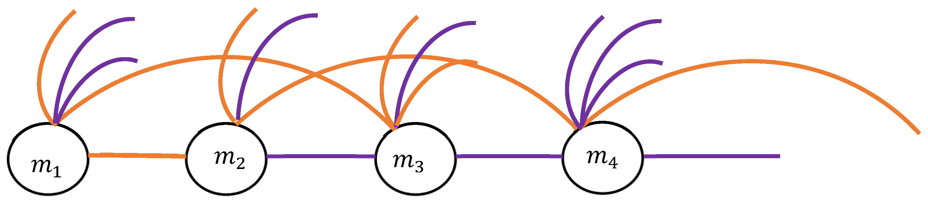
2.3. Kinematic Graphs Emerging from the Motion of Multi-Particle Systems

Consider the kinematic graph emerging from the motion of five particles, $m_i,i=1,\dots ,5$, presented in Figure 5. The system of the motile particles is not necessarily 2D; it may constitute a 3D set of motile particles. The coloring of the edges is defined by Equations (2) and (3). We consider the hypothetic coloring presented in Figure 5. As was already demonstrated, the coloring is non-transitive. No monochromatic triangle is recognized in the graph. Indeed, this result is consistent with the Ramsey theory: $R\left(\mathrm{3,3}\right)=6.$

Thus, we conclude that a physical situation exists for the system comprising five particles in which the triad of converging particles or particles moving away from each other/remaining at the same distance from each other will be absent in the system built of five motile point masses.

Now, we address a system built of six point motile masses (it also may be a 3D system of particles).

We address the hypothetical coloring, described using Equations (2) and (3), shown in Figure 6. Monochromatic orange triangles $\left(m_1,m_3,m_5\right)$ and $\left(m_2,m_4,m_6\right)$ are recognized in the graph. This means that within the triads of point masses $\left(m_1,m_3,m_5\right)$ and $\left(m_2,m_4,m_6\right),$ the particles move away from each other or perhaps remain at the same distance from each other. Moreover, the Ramsey theorem states that within any graph describing the motion of six particles, we will inevitably find at least one monochromatic triangle. In other words, we always will find a triangle built of three particles in which the particles will converge or move away from each other/remain at the same distance. Indeed, the Ramsey number $R\left(\mathrm{3,3}\right)=6.$ It should be emphasized that the Ramsey theorem does not predict what kind/color of triangles will appear in a graph, and this should be established using a brute-force method based on an analysis of the dynamics of the addressed system [10,11,12,13].

The graphs depicted in Figure 3, Figure 4, Figure 5 and Figure 6 are temporal graphs, and their coloring will change with time [22,23,24]. The total number of mono-colored triangles within the given graph is supplied by

$$n_{tot}\left(t\right)=n_{orange}\left(t\right)+n_{violet}\left(t\right),$$

(5)

where ${\mathit{n}}_{\mathit{o}\mathit{r}\mathit{a}\mathit{n}\mathit{g}\mathit{e}}\left(\mathit{t}\right)\mathrm{a}\mathrm{n}\mathrm{d}{\mathit{n}}_{\mathit{v}\mathit{i}\mathit{o}\mathit{l}\mathit{e}\mathit{t}}\left(\mathit{t}\right)$ are the time-dependent numbers of orange and violet monochromatic triangles in a given graph. It is noteworthy that ${\mathit{n}}_{\mathit{t}\mathit{o}\mathit{t}}\left(\mathit{t}\right),{\mathit{n}}_{\mathit{o}\mathit{r}\mathit{a}\mathit{n}\mathit{g}\mathit{e}}\left(\mathit{t}\right)\mathrm{a}\mathrm{n}\mathrm{d}{\mathit{n}}_{\mathit{v}\mathit{i}\mathit{o}\mathit{l}\mathit{e}\mathit{t}}\left(\mathit{t}\right)$ are frame-independent.

The introduced Ramsey approach may be generalized to swarms built of large number of particles. Consider a swarm built of eighteen particles. The coloring of the graph corresponding to this system is defined by Equations (2) and (3). Tetrads of converging particles or particles moving away from each other will necessarily appear in this swarm. This conclusion emerges from the fact that the Ramsey number $\mathit{R}\left(\mathbf{4},\mathbf{4}\right)=\mathbf{18}.$ It is noteworthy that the calculation of “large” Ramsey numbers remains an unsolved problem.

2.4. Generalization for Infinite Systems of Material Points

Now, consider an infinite but countable system of moving material points/particles $\left\{{\mathit{m}}_1,{\mathit{m}}_2,\dots {\mathit{m}}_{\mathit{n}}\dots \right\}$. The particles form the vertices of an infinite bi-colored graph. The vertices/particles are connected with an orange link when the particles move away from each other/remain at the same distance in the course of their motion (in other words, Equation (2) is true). The vertices/particles are connected with a violet link when the particles converge (Equation (3) is correct). Figure 7 represents a graph corresponding to the instant photo of the motion. According to the infinite Ramsey theorem, an infinite monochromatic (violet or orange) clique will necessarily appear in the graph [13,29].

Let us rigorously formulate the infinite Ramsey theorem.

Let ${\mathit{K}}_{\mathit{\omega }}$ denote the complete colored graph on the vertex set N. For every $\mathit{\zeta }>\mathbf{0}$, if we color the edges of ${\mathit{K}}_{\mathit{\omega }}$ with $\mathit{\zeta }$ distinguishable colors, then an infinite monochromatic clique must be present [13]. An infinite monochromatic clique in a colored graph is a subset of vertices that are all pairwise-adjacent (i.e., that form a clique) and whose edges are all the same color in a given edge coloring of the graph. The infinite Ramsey theorem re-formulates the seminal Dirichlet pigeonhole principle, which states that if n pigeonholes exist containing $\mathit{n}+\mathbf{1}$ pigeons, one of the pigeonholes necessarily must contain at least two pigeons [13]. Thus, a monochromatic clique will necessarily appear in the kinematic graph shown in Figure 7. And. again, the coloring of the graph is time-dependent but frame-independent. The infinite Ramsey theorem does not predict the exact color of the monochromatic clique.

3. Discussion

We introduced the mathematic procedure applicable to the analysis of the motion of material points/particles. The mathematical scheme is based on the theory of colored graphs, and it converts an instant photo of the motion into a bi-colored Ramsey graph [8,9,10,11,12,13,30]. The particles serve as the vertices of the graph. The coloring of the edges/links is based on the time dependence of the distance between the particles. If the distance between a pair of particles grows with time in the course of their motion (or remains the same), the edge is colored with an orange color (the vertices/particles are seen as “strangers” [30]); if the distance between the particles decreases with time, the edge is colored in violet (the vertices/particles are seen as “friends”). Thus, a complete bi-colored temporal graph emerges. The coloring is time-dependent; however, it is frame-independent. Let us discuss the application of the introduced Ramsey approach:

(i)

The introduced Ramsey kinematics may be useful for the analysis of turbulence. Turbulence has been investigated for a long time within the Eulerian approach [30]. However, the fundamental mechanisms of turbulent flows, as well as their mixing and transport properties, can be more naturally understood within the Lagrangian paradigm [31,32,33]. In particular, the relative separation of a pair of tracers is closely related to the growth of a blob of a passive scalar in a turbulent flow [31,32,33]. Our results demonstrate that in any set of six tracers, we will always find three which converge or move away from each other. And, consequently, in any set of 18 tracers, there will be always present the tetrad of tracers which converge or move away from each other [31,32,33].

(ii)

The developed approach may be useful for analyses of the strain of a deformable body (not necessarily elastic). Consider the deformable body depicted in Figure 8. Points $\left\{\mathrm{1,2}\dots 6\right\}$ are fixed within the body, and then the stress $\sigma$ is applied (see Figure 8). The points are displaced relative to other. We connect the points with links; the coloring of the links is described using Equations (2) and (3).

Monochromatic orange triangles $\left\{\mathrm{1,3.5}\right\}$ and $\left\{\mathrm{2,4},6\right\}$ are recognized in the graph shown in Figure 8. It should be emphasized that the appearance of at least one monochromatic triangle in the graph is independent of the kind of deformation, i.e., the deformation may be elastic or plastic.

(iii)

The analysis introduced may be applied to the study of the motion of elementary particles. For example, the decay of an excited ²⁴Mg nucleus into six α particles from a selection of central ¹²C+ ¹²C reactions at a 95 MeV beam energy was studied [34]. The kinematic graph emerging from the motion of six motile particles, depicted in Figure 6, is applicable to an analysis of the motion of six α particles.

(iv)

The study of the motion of particles and droplets, their clusters and their swarms [35,36,37].

(v)

Celestial mechanics. It is interesting that ancient astronomers distinguished six planets, namely Mercury, Earth, Venus, Mars, Jupiter, and Saturn [38].

(vi)

The study of the motion of swarms of bacteria, when the formation of triads and tetrads of bacteria is important [39].

In our future investigations, we plan to cover the following:

(i)

An extension to the suggested approach to relativistic particles.

(ii)

An extension of the approach to the motion of deformable bodies.

(iii)

An extension of the approach to the motion of large numbers of particles (which may be separated into subsets of six particles).

(iv)

The development of the a-colored kinematic Ramsey approach: the first kind of link connects particles which converge; the second kind of link connects particles which move away from each other; and the third kind of link connects particles which are at rest relative to one another.

4. Conclusions

We conclude that graph theory supplies powerful tools for the analysis of the motion of systems of material points/particles. We have completely neglected the details of the interaction between the particles, and we based our analysis on the time dependence of the distance between the particles, thus adopting a pure kinematic approach. The distance between the motile particles, numbered i and k, denoted as $r_{ik}\left(t\right)$, may grow with time/remain the same, i.e., ${\displaystyle \frac{d{r}_{ik}}{dt}}\ge 0$, or alternatively, it may decrease with time in the course of the motion of the particles, i.e., ${\displaystyle \frac{d{r}_{ik}}{dt}}<0$ holds. The motile particles themselves serve as the vertices of the graph. The distinction in the temporal behavior of the function $r_{ik}\left(t\right)$, prescribed by the sign of its derivative, enables bi-coloring of the edges linking the particles. Particles moving away from each other/remaining at the same distance are connected with an orange link; the converging particles are, in turn, connected with a violet link. We have demonstrated that the suggested coloring scheme is not transitive. This is important in view of the application of Ramsey graph theory to the analysis of a complete, bi-colored, complete, temporal graph emerging from the motion of particles. The Ramsey number $R\left(\mathrm{3,3}\right)=6.$ This means that any physical system built of six particles will correspond a bi-colored, complete graph drawn according to the aforementioned mathematical scheme, which will contain at least one monochromatic triangle. In other words, the addressed physical system will necessarily contain at least one triad of particles which move away from each other/remain in the same system or converge. The proposed scheme completely ignores the peculiarities of the Hamiltonian/Lagrangian properties of the system. It is based on an analysis of the temporal behavior of the distances between the particles. The introduced mathematical scheme is time-dependent, and the temporal bi-colored graph corresponds to the system [23,24,25,40]. However, the emerging graph is frame-independent. The number of monochromatic triangles is frame-independent. The reported results illustrate the main result supplied by Ramsey theory; namely, total chaos is impossible. In sufficiently large structures, the emergence of ordered sub-structures (in our case, mono-colored triangles) is inevitable. The extension of the suggested approach to the analysis of systems built of an arbitrary number of point masses is straightforward. However, the calculation of large Ramsey numbers remains a challenging and unsolved mathematical task. Generalization of the suggested approach to infinite systems of particles is reported. The relativistic extension of the suggested method should be developed.

References

1. Wigner, E.P. The Unreasonable Effectiveness of Mathematics in the Natural Sciences. In Mathematics and Science; World Scientific: Singapore, 1990; pp. 291–306. [Google Scholar]
2. Grinbaum, A. The effectiveness of mathematics in physics of the unknown. Synthese 2019, 196, 973–989. [Google Scholar] [CrossRef]
3. Plotnitsky, A. On the Reasonable and Unreasonable Effectiveness of Mathematics in Classical and Quantum Physics. Found. Phys. 2011, 41, 466–491. [Google Scholar] [CrossRef]
4. Bondy, J.A.; Murty, U.S.R. Graph Theory; Springer: New York, NY, USA, 2008. [Google Scholar]
5. Bollobás, B. Modern Graph Theory; Springer: Berlin, Germany, 2013; Volume 184. [Google Scholar]
6. Kosowski, A.; Manuszewski, K. Classical coloring of graphs. Contemp. Math. 2008, 352, 1–20. [Google Scholar]
7. Kano, M.; Li, X. Monochromatic and Heterochromatic Subgraphs in Edge-Colored Graphs—A Survey. Graphs Comb. 2008, 24, 237–263. [Google Scholar] [CrossRef]
8. Chartrand, G.; Chatterjee, P.; Zhang, P. Ramsey chains in graphs. Electron. J. Math. 2023, 6, 1–14. [Google Scholar] [CrossRef]
9. Chartrand, G.; Zhang, P. New directions in Ramsey theory. Discret. Math. Lett. 2021, 6, 84–96. [Google Scholar]
10. Graham, R.L.; Rothschild, B.L.; Spencer, J.H. Ramsey Theory, 2nd ed.; Wiley-Interscience Series in Discrete Mathematics and Optimization; John Wiley & Sons, Inc.: New York, NY, USA, 1990; pp. 10–110. [Google Scholar]
11. Graham, R.; Butler, S. Rudiments of Ramsey Theory, 2nd ed.; American Mathematical Society: Providence, RI, USA, 2015; pp. 7–46. [Google Scholar]
12. Di Nasso, M.; Goldbring, I.; Lupini, M. Nonstandard Methods in Combinatorial Number Theory, Lecture Notes in Mathematics; Springer: Berlin, Germany, 2019; Volume 2239. [Google Scholar]
13. Katz, M.; Reimann, J. Introduction to Ramsey Theory: Fast Functions, Infinity, and Metamathematics; Student Mathematical Library; American Mathematical Society: Providence, RI, USA, 2018; Volume 87, pp. 1–34. [Google Scholar]
14. Erdős, P. Solved and unsolved problems in combinatorics and combinatorial number theory. Congr. Numer. 1981, 32, 49–62. [Google Scholar]
15. Conlon, D.; Fox, J.; Sudakov, B. Recent developments in graph Ramsey theory. Surv. Comb. 2015, 424, 49–118. [Google Scholar]
16. de Gois, C.; Hansenne, K.; Gühne, O. Uncertainty relations from graph theory. Phys. Rev. A 2023, 107, 062211. [Google Scholar] [CrossRef]
17. Xu, Z.-P.; Schwonnek, R.; Winter, A. Bounding the Joint Numerical Range of Pauli Strings by Graph Parameters. PRX Quantum 2024, 5, 020318. [Google Scholar] [CrossRef]
18. Hansenne, K.; Qu, R.; Weinbrenner, L.T.; de Gois, C.; Wang, H.; Ming, Y.; Yang, Z.; Horodecki, P.; Gao, W.; Gühne, O. Optimal overlapping tomography. arXiv 2024, arXiv:2408.05730. [Google Scholar]
19. Wouters, J.; Giotis, A.; Kang, R.; Schuricht, D.; Fritz, L. Lower bounds for Ramsey numbers as a statistical physics problem. J. Stat. Mech. 2022, 2022, 0332. [Google Scholar]
20. Shvalb, N.; Frenkel, M.; Shoval, S.; Bormashenko, E. Dynamic Ramsey Theory of Mechanical Systems Forming a Complete Graph and Vibrations of Cyclic Compounds. Dynamics 2023, 3, 272–281. [Google Scholar] [CrossRef]
21. Frenkel, M.; Shoval, S.; Bormashenko, E. Fermat Principle, Ramsey Theory and Metamaterials. Materials 2023, 16, 7571. [Google Scholar] [CrossRef]
22. Bormashenko, E.; Shvalb, N. A Ramsey-Theory-Based Approach to the Dynamics of Systems of Material Points. Dynamics 2024, 4, 845–854. [Google Scholar] [CrossRef]
23. Michail, O. An introduction to temporal graphs: An algorithmic perspective. Internet Math. 2016, 12, 239–280. [Google Scholar] [CrossRef]
24. Michail, O.; Spirakis, P.G. Traveling salesman problems in temporal graphs. Theor. Comput. Sci. 2016, 634, 1–23. [Google Scholar]
25. Erlebach, T.; Hoffmann, M.; Kammer, F. On temporal graph exploration. J. Comput. Syst. Sci. 2021, 119, 1–18. [Google Scholar]
26. Choudum, S.A.; Ponnusamy, B. Ramsey numbers for transitive tournaments. Discret. Math. 1999, 206, 119–129. [Google Scholar] [CrossRef]
27. Gilevich, A.; Shoval, S.; Nosonovsky, M.; Bormashenko, E. Converting Tessellations into Graphs: From Voronoi Tessellations to Complete Graphs. Mathematics 2024, 12, 2426. [Google Scholar] [CrossRef]
28. Choudum, S.A.; Ponnusamy, B. Ordered Ramsey numbers. Discret. Math. 2002, 247, 79–92. [Google Scholar]
29. Li, Y.; Lin, Q. Elementary Methods of the Graph Theory; Applied Mathematical Sciences; Springer: Cham, Switzerland, 2020; pp. 3–44. [Google Scholar]
30. Ramsey, F.P. On a Problem of Formal Logic. In Classic Papers in Combinatorics; Gessel, I., Rota, G.C., Eds.; Modern Birkhäuser Classics; Birkhäuser: Boston, MA, USA, 2009; pp. 264–286. [Google Scholar]
31. Landau, L.D.; Lifshitz, E.M. Fluid Mechanics; Pergamon Press: Oxford, UK, 1987. [Google Scholar]
32. Polanco, J.I.; Arun, S.; Naso, A. Multiparticle Lagrangian statistics in homogeneous rotating turbulence. Phys. Rev. Fluids 2023, 8, 034602. [Google Scholar]
33. Salazar, J.P.L.C.; Collins, L.R. Two-Particle Dispersion in Isotropic Turbulent Flows. Ann. Rev. Fluid Mech. 2009, 41, 405–432. [Google Scholar]
34. Morell, L.; Bruno, M.; D’Agostino, M. Full disassembly of excited 24Mg into six α particles. Phys. Rev. C 2019, 99, 054610. [Google Scholar]
35. Shaffer, F.; Hay, R.; Karri, S.B.R.; Knowlton, T. Particle clusters in and above fluidized beds. Powder Technol. 2010, 203, 3–11. [Google Scholar]
36. Fedorets, A.A.; Bormashenko, E.; Dombrovsky, L.A.; Nosonovsky, M. Droplet clusters: Nature-inspired biological reactors and aerosols. Philos. Trans. R. Soc. A 2019, 377, 20190121. [Google Scholar]
37. Nourhani, A. Biomimetic swarm of active particles with coupled passive-active interactions. Soft Matter 2025. online ahead of print. [Google Scholar]
38. Motz, L.; Weaver, J.H. The Planets and Their Motions. In The Unfolding Universe; Springer: Boston, MA, USA, 1989. [Google Scholar]
39. Samantaray, K.; Mishra, S.R.; Purohit, G.; Mohanty, P.S. AC Electric Field Mediated Assembly of Bacterial Tetrads. ACS Omega 2020, 5, 5881–5887. [Google Scholar]
40. Wang, Y.; Yuan, Y.; Ma, Y.; Wang, G. Time-Dependent Graphs: Definitions, Applications, and Algorithms. Data Sci. Eng. 2019, 4, 352–366. [Google Scholar]
Figure 1. The simplest system built of a pair of point masses m 1 ,   m 2   is depicted. The Cartesian coordinates of the masses are shown.
Dynamics 05 00011 g001
Figure 2. The coloring procedure is illustrated. (A) Particles m 1 and m 2 move away from each other or remain at the same distance, and d r 12 t d t 0 is true. The particles are connected with an orange link. (B) Particles m 1 and m 2 converge, and d r 12 t d t < 0 occurs. The particles are connected with a violet link. Green arrows illustrate the direction of the particles’ motion.
Dynamics 05 00011 g002
Figure 3. The coloring for the motion of the triad of particles   m 1 ,     m 2 , and m 3 is demonstrated. The green arrows depict the direction of the particles’ motion. The coloring is non-transitive.
Dynamics 05 00011 g003
Figure 4. Possible coloring for the motion of the triad of particles   m 1 ,   m 2 , and m 3 is demonstrated. The green arrows depict the direction of the particle motion. (A) The resulting triangle is bi-colored. (B) The resulting triangle is mono-colored in violet. If the particles move away from each other or remain at the same distance, they are connected with an orange link; when the particles converge they are connected with a violet link.
Dynamics 05 00011 g004
Figure 5. Kinematic graph emerging from the motion of five particles, m i ,   i = 1 , , 5 . No monochromatic triangle is recognized in this graph. If the particles move away from each other or remain at the same distance, they are connected with an orange link; when the particles converge, they are connected with a violet link.
Dynamics 05 00011 g005
Figure 6. Kinematic graph emerging from the motion of six motile particles, m i ,   i = 1 , , 6 . Monochromatic orange triangles m 1 , m 3 , m 5 and m 2 , m 4 , m 6 are recognized in the graph.
Dynamics 05 00011 g006
Figure 7. An infinite but countable system of moving material points/particles m 1 , m 2 , m n is depicted. The particles form the vertices of an infinite, bi-colored graph. The vertices/particles are connected with an orange link when the particles move away from each other/remain at the same distance. The vertices/particles are connected with the violet link when the particles converge. An infinite monochromatic (violet or orange) clique will necessarily appear in the graph.
Dynamics 05 00011 g007
Figure 8. Six points labeled 1 , , 6 located within the deformable body are depicted. Stress σ is applied. Points are displaced under the deformation, and the color of the links connecting the points is established using Equations (2) and (3). Monochromatic orange triangles 1,3 , 5 and 2,4 , 6 are recognized in the graph. . If the points move away from each other or remain at the same distance, they are connected with an orange link; when the points converge, they are connected with a violet link.
Dynamics 05 00011 g008
Disclaimer/Publisher’s Note: The statements, opinions and data contained in all publications are solely those of the individual author(s) and contributor(s) and not of MDPI and/or the editor(s). MDPI and/or the editor(s) disclaim responsibility for any injury to people or property resulting from any ideas, methods, instructions or products referred to in the content.