On Solutions of the Third-Order Ordinary Differential Equations of Emden-Fowler Type

Abstract

For a linear ordinary differential equation (ODE in short) of the third order, results are presented that supplement the theory of conjugate points and extremal solutions by W. Leighton, Z. Nehari, M. Hanan. It is especially noted the sensitivity of solutions to the initial data, which makes their numerical study difficult. Similar results were obtained for the third-order nonlinear equations of the Emden-Fowler type.

1. Introduction

Ordinary differential equations are widely used in science, mathematical modeling, physics, biology, and other fields. For students, this is another stage of mathematical learning, after elementary algebra, geometry and different types of equations. Differential equations, considered as models of natural and industrial processes, can catch dynamics, and show the development, and evolution of modeled processes. The theory of ordinary differential equations, when taught to students, starts with linear ones. There is well developed theory, which provides almost exhaustive answers to questions and problems concerning linear ODE with constant coefficients. For equations with coefficients, depending on an independent variable, the theory provides knowledge of the structure of a set of solutions and definitions of the main properties of solutions. When passing to nonlinear ODE, many principal concepts are lost, for instance, the superposition principle and extendability of solutions to infinity (for regular linear equations, without singularities). For practical purposes, numerical analysis often can be performed, and it is sufficient to find solutions. However, sensitive dependence of solutions to the initial data occurs often in practical problems and in theoretical studies of nonlinear ODE.

It can make difficult or even impossible the numerical study. In this article we attract attention to the occurrence of this and similar problems even in the study of relatively simple linear and nonlinear ODE. For this, we have chosen the theory of conjugate points, as developed in the works of W. Leighton, Z. Nehari [1], M. Hanan [2], T. Sherman [3], V. Kondrat’ev [4,5], etc. We would like to mention also the works by S. Smirnov [6,7], who has found interesting properties of solutions of the third order nonlinear ODE and applications to boundary value problems, as well as findings of I. Astashova et al. [8], concerning the asymptotic properties of solutions. The third order equations with deviating arguments were considered in [9,10]. The sensitive dependence of solutions on the initial data is of permanent interest [11].

A few words about the conjugate points. The first order linear ODE of the type $x^{\prime }=a\left(t\right)x+b\left(t\right)$ have no surprises, if the coefficients are continuous functions. The second order linear ODE of the form $x^{″}+p\left(t\right)x^{\prime }+g\left(t\right)x=f\left(t\right)$ are more intriguing. They can exhibit oscillatory behavior of solutions, and a lot of problems arise. It is firm, however, that the oscillatory behavior of solutions is intuitively connected to zeros, and the rate of oscillation can be measured by the number of zeros.

When passing to linear equations of order three, and higher, the notion of a zero of a solution becomes more complicated. There are multiple zeros, that is, zeros for a solution, and some of its derivatives. Nevertheless, the rate of oscillation of some classes of linear ODE of higher orders can be measured, introducing the notion of conjugate points. Definitions for the third order linear equations are provided below, following the work by M. Hanan, who, in turn, used the theory of conjugate points for classes of linear equations of order four, developed earlier by W. Leighton and Z. Nehari. The definition of conjugate points for the third order linear equations seems to be tricky since it uses the extremality property of zeros and leads to the concept of an extremal solution. Further analysis of these definitions simplifies the problem and results in the efficient criteria for finding conjugate points, as in Theorem 1. So conjugate points for some classes of equations of order higher than two, play the same role as ordinary zeros play for the second order equations. So there are conjugate points, and there are the so called extremal solutions, attributed to them. In this article we provide some additional information on the theory of conjugate points for linear ODE of order three. The structure of extremal solutions is revealed, and their remarkable properties are discussed. Namely, the mutual location of extremal solutions is described and, among others, the sensitive dependence of extremal solutions on the initial conditions is discussed.

The second part of the article concerns the nonlinear equations of the Emden-Fowler type, which in some sense, behave similarly to linear equations, considered in Section 2 and Section 3. Both the analytical approach and the numerical study are used. Some results in the literature, concerning nonlinear equations, are reminded and their consequences to extremal solutions for the Emden-Fowler type equations are formulated.

Consider the linear equation

$$x^{‴}=p\left(t\right)x,$$

(1)

where $p\left(t\right)$ is a positive valued continuous function. This equation was studied by many authors; we will mention the works [2,4,5], books [12,13,14,15].

The theorem by M. Hanan [2] states that there exist special solutions $x_i\left(t\right)$ with

$$x\left(0\right)=0,x^{\prime }\left(0\right)>0,x^{″}\left(0\right)<0,$$

(2)

which have a double zero at some point ${\eta }_i>0.$ These points form ascending sequence and are called by conjugate points to $t=0$ for equations of the form (1). These points can be visualized considering the equation

$$x^{‴}=px,p=\mathit{constant}>0.$$

(3)

We recall the structure of a set of solutions to equations of the type (1) and discuss what happens under passage to nonlinear equations

$$x^{‴}=p{\left|x\right|}^{\gamma }x,\gamma >0.$$

(4)

2. Linear Equation

W. Leighton and Z. Nehari [1] have investigated oscillatory properties of solutions to linear equations of the form

$$x^{\left(4\right)}=p\left(t\right)x,$$

(5)

where $p\left(t\right)$ is a continuous positive (or negative) valued function. To measure the rate of oscillation of Equation (5) they introduced the notion of conjugate points. Similar task was accomplished by M. Hanan [2] who studied the third order linear differential equations

$$x^{‴}=p\left(t\right)x+q\left(t\right)x^{\prime }+r\left(t\right)x^{″}$$

(6)

with continuous coefficients. The conjugate points for the Equation (6) were introduced in the following way. Suppose that Equation (6) has a solution $x\left(t\right)$ which vanishes at $t=a$ and has at least $n+2$ zeros $a_1,\dots ,a_{n+2}$ in $(a,+\infty ).$ Then ${\eta }_n$ is called ([2], p. 920) the n-th conjugate point to $t=a$ with respect to Equation (6) if it is a smallest possible value of $a_{n+2}$ as $x\left(t\right)$ ranges over all possible solutions of (6) for which $x\left(a\right)=0.$ Due to this extremality property of a conjugate point the solution which produces the n-th conjugate point is called the n-th extremal solution.

To get description of conjugate points the following characterization of linear equations was introduced.

Definition 1 

([2]). Equation (6) is said to be of Class I if any its solution $x\left(t\right)$ for which $x\left(a\right)=x^{\prime }\left(a\right)=0$ and $x^{″}\left(a\right)>0$ is positive for $t<a$.

Definition 2 

([2]). Equation (6) is said to be of Class II if any its solution $x\left(t\right)$ for which $x\left(a\right)=x^{\prime }\left(a\right)=0$ and $x^{″}\left(a\right)>0$ is positive for $t>a$.

There are equations that belong to both classes (for instance, $x^{‴}=0$) and there exist equations (for example, $x^{‴}=-x^{\prime }$) that are neither of Class I nor of Class II.

Several criteria for Equation (6) to be of Class I or Class II are given in [2,12,13] of which we mention only the simplest one. Namely, Equation (1) is of Class I if $p\left(t\right)<0$ and of Class II if $p\left(t\right)>0.$

The characterization of conjugate points for equations of Class I and Class II was given by M. Hanan [2] (theorems 2.6, 2.7 and 4.4).

Theorem 1. 

Conjugate points ${\eta }_i\left(a\right)$ of an equation of Class I are the zeros (which are simple) of the so called principal solution, that is the solution $x\left(t\right)$ which satisfies the initial conditions

$$x\left(a\right)=x^{\prime }\left(a\right)=0,x^{″}\left(a\right)=1.$$

(7)

Conjugate points ${\eta }_i\left(a\right)$ (if any) of an equation of Class II form ascending sequence

$$a<{\eta }_1<\dots <{\eta }_n<\dots$$

The respective extremal solutions $x_i\left(t\right)$ ($i=1,\dots$) have a simple zero at $t=a,$ double zero at ${\eta }_i$ (that is, $x_i\left({\eta }_i\right)=x^{\prime }\left({\eta }_i\right)=0$) and exactly $i-1$ simple zeros in $(a,{\eta }_i\left(a\right)).$

The first part of the above statement is Theorem 2.6 in [2] and the second one is Theorem 2.7 in the same source.

From now consider Equation (1) with positive $p\left(t\right).$ They belong to Class II. It is an easy matter to show that nontrivial solutions of (1) with the initial conditions $x\left(a\right)=0,$$x^{\prime }\left(a\right)\ge 0,$$x^{″}\left(a\right)\ge 0$ or $x\left(a\right)=0,$$x^{\prime }\left(a\right)\le 0,$$x^{″}\left(a\right)\le 0$ do not vanish for $t>a.$ So any extremal solution $x_i\left(t\right)$ satisfies (up to multiplication by $-1$) the conditions $x_i\left(a\right)=0,$ $x_i^{\prime }\left(a\right)>0,$$x_i^{″}\left(a\right)<0.$ It is convenient to attribute the angle ${\varphi }_i=arctan\frac{x_i^{″}\left(a\right)}{x_i^{\prime }\left(a\right)}$ to the extremal solution.

Studying the properties of these angles have led us to the following result.

Theorem 2. 

For a linear equation of Class II:

(1) the angles ${\varphi }_i\left(a\right)$ corresponding to the extremal solutions $x_i\left(t\right)$ are arranged as

$$-\pi /2<{\varphi }_2<{\varphi }_4<\dots <{\varphi }_{2i}<\dots <{\varphi }_{2i+1}<\dots <{\varphi }_3<{\varphi }_1<0;$$

(8)

(2) solutions $x\left(t\right),$ defined by the initial conditions

$$x\left(a\right)=0,\varphi \in ({\varphi }_{2i},{\varphi }_{2i+2}),\varphi =arctan\frac{x^{″}\left(a\right)}{x^{\prime }\left(a\right)}i=0,1,2,\dots$$

have for $t>a$ exactly $2i+2$ simple zeros, and solutions defined by the initial conditions

$$x\left(a\right)=0,\varphi \in ({\varphi }_{2i+1},{\varphi }_{2i-1}),i=0,1,2,\dots$$

have for $t>a$ exactly $2i+1$ simple zeros (${\varphi }_0$ means $-\frac{\pi }{2}$ and ${\varphi }_{-1}$ is set to zero).

Proof. 

We consider extremal solutions $x_k\left(t\right),$ for which the first order derivative at $t=a$ is positive, and the second order derivative is negative. Taking into account that all zeros of an extremal function $x_k\left(t\right)$ in the interval $(a,{\eta }_k)$ are simple, and $x_k\left(t\right)$ changes sign at each of them, we conclude that $x_k\left(t\right)$ is positive for $t>{\eta }_k,$ if k is odd, and it is negative for the same t if k is even.

Let us compare two extremal solutions with odd numbers. We wish to show that ${\varphi }_{2k+1}>{\varphi }_{2l+l}$ if $k<l.$ Suppose that $x_{2k+1}^{\prime }\left(a\right)=x_{2l+1}^{\prime }\left(a\right)$ and comparison is made only for the second order derivatives at $t=a.$ This is possible always, since extremal solutions can be multiplied by a constant, and this does not change the corresponding angle $\varphi \left(a\right).$ By Theorem 1, ${\eta }_{2k+1}<{\eta }_{2l+1}.$ For $t>{\eta }_{2l+1}$ both extremal functions are positive. Let us show that the assumption $x_{2l+1}^{″}\left(a\right)>x_{2k+1}^{″}\left(a\right)$ or, which is the same, ${\varphi }_{2k+1}<{\varphi }_{2l+l},$ leads to contradiction. Note, that the case $x_{2l+1}^{″}\left(a\right)=x_{2k+1}^{″}\left(a\right)$ is excluded, since then both extremal solutions must coincide, by the unique solvability of the Cauchy problems. Consider the difference $y=x_{2l+1}-x_{2k+1}.$ The function $y\left(t\right)$ is a solution of the same equation with the initial conditions $y\left(a\right)=0,$$y^{\prime }\left(a\right)=0,$$y^{″}\left(a\right)>0.$ Therefore $y\left(t\right)>0$ for $t>a,$ since the equation is of Class II, and any solution with positive $y^{″}\left(a\right)$ is positive to the right of a double zero. However, this contradicts the fact that $y\left({\eta }_{2l+1}\right)=x_{2l+1}\left({\eta }_{2l+1}\right)-x_{2k+1}\left({\eta }_{2l+1}\right)<0.$

It can be proved similarly, that ${\varphi }_{2l}>{\varphi }_{2k}$ if $l>k.$

Let us show now, that ${\varphi }_{2k-1}>{\varphi }_{2l}$ for any positive integers k and $l.$ We assume that $x_{2k-1}^{\prime }\left(a\right)=x_{2l}^{\prime }\left(a\right)$ and $x_{2k-1}^{″}\left(a\right)<x_{2l}^{″}\left(a\right).$ Consider the function $y=x_{2l}-x_{2k-1}.$ Since $y\left(t\right)$ has a double zero at $t=a$ and $y^{″}\left(a\right)>0,$ by assumption, $y\left(t\right)$ is positive for $t>a.$ Two cases are possible. The first one, $2l>2k-1.$ Then ${\eta }_{2l}>{\eta }_{2k-1}.$ One has that $y\left({\eta }_{2l}\right)=x_{2l}\left({\eta }_{2l}\right)-x_{2k-1}\left({\eta }_{2l}\right)<0.$ This is in contradiction with positivity of $y\left(t\right)$ for $t>a.$ The second possible case, $2l<2k-1.$ Then ${\eta }_{2l}<{\eta }_{2k-1}.$ One has that $y\left({\eta }_{2k-1}\right)=x_{2l}\left({\eta }_{2k-1}\right)-x_{2k-1}\left({\eta }_{2k-1}\right)<0.$ The contradiction with positivity of $y\left(t\right)$ for $t>a$ is obtained again.

The first statement of the theorem is proved.

Let us pass to the second statement. Consider a solution $x\left(t\right)$ which vanishes at $t=a$ and is defined by the angle $\varphi \in ({\varphi }_{2k-1}, {\varphi }_{2k+1}),$ $k=1,2,\dots$ Let us compare this solution with the extremal solutions $x_{2k-1}$ and $x_{2k+1}$ provided that the first derivatives of all three solutions at $t=a$ are equal. The functions $u=x_{2k-1}-x$ and $v=x-x_{2k+1}$ are positive for $t>a.$ It follows that $x_{2k-1}\left(t\right)>x\left(t\right)>x_{2k+1}\left(t\right)$ for $t>a.$ Denote simple zeros of the function $x_{2k-1}$ in the interval $(a,{\eta }_{2k-1})$ by ${\tau }_i$ and simple zeros of the function $x_{2k+1}$ by $t_i.$ Consider the relative locations of zeros ${\tau }_i$ and $t_j.$ For even i the function $x_{2k-1}$ is positive in $({\tau }_i,{\tau }_{i+1}),$ and the function $x_{2k+1}$ is positive in $(t_i,t_{i+1})$ (we accept that ${\tau }_0=t_0=a$). Show that ${\tau }_i<t_i<t_{i+1}<{\tau }_{i+1}$ for $i=0,2,4,\dots$ If this is not the case, then there exists an interval $({\tau }_i,{\tau }_{i+1})$ with even i such that $x_{2k+1}\left(t\right)<0$ for $t\in [{\tau }_i,{\tau }_{i+1}].$ Then, by Lemma 2 in [1], there exists a number $\mu$ such that the function $z\left(t\right)=x_{2k-1}\left(t\right)+\mu x_{2k+1}\left(t\right)$ has a double zero in the interval $({\tau }_i,t_{i+1}).$ Since the function $z\left(t\right)$ is a solution of Class II, it does not vanish for $t>t_{i+1}.$ On the other hand, the number $\mu$ is positive, since otherwise $z=x_{2k-1}+\mu x_{2k+1}>0$ for $t\in ({\tau }_i,t_{i+1}),$ what contradicts the existence of a zero in this interval. Then $z\left({\eta }_{2k-1}\right)=x_{2k-1}\left({\eta }_{2k-1}\right)+\mu x_{2k+1}\left({\eta }_{2k-1}\right)<0$ because the first addend is zero, and $x_{2k+1}\left({\eta }_{2k-1}\right)<x_{2k-1}\left({\eta }_{2k-1}\right)<0.$ But $z\left({\eta }_{2k+1}\right)=x_{2k-1}\left({\eta }_{2k+1}\right)+\mu x_{2k+1}\left({\eta }_{2k+1}\right)>0$ since the second addend is zero, and $x_{2k-1}\left(t\right)$ is positive for $t>{\eta }_{2k-1}.$ Therefore, the function $z\left(t\right)$ changes sign in the interval $({\eta }_{2k-1},{\eta }_{2k+1}),$ which lies to the right of $t=t_{i+1}.$ The obtained contradiction means that any interval $({\tau }_i,t_{i+1}),$ where the function $x_{2k-1}$ is positive, contains a subinterval $(t_i,t_{i+1}),$ where the function $x_{2k+1}\left(t\right)$ is positive. We have proved that zeros of the functions $x_{2k-1}$ and $x_{2k+1}$ are arranged as

$$a<t_1<{\tau }_1<{\tau }_2<t_2<t_3<\dots <{\tau }_{2k-2}<t_{2k-2}<t_{2k-1}<t_{2k}<t_{2k+1}<{\eta }_{2k+1}.$$

It follows from the inequalities $x_{2k-1}\left(t\right)<x\left(t\right)<x_{2k+1}\left(t\right),$ which are valid for $t>a,$ that in any interval $(t_1,{\tau }_1),\dots ,({\tau }_{2k-2},t_{2k-2}),(t_{2k-1},{\eta }_{2k-1})$ there exists a zero of $x\left(t\right).$ Thus the function $x\left(t\right)$ has in the interval $(a,{\eta }_{2k-1})$ totally $1+(2k-1)=2k$ zeros, and $x\left({\eta }_{2k-1}\right)<0.$ It follows that there exists an extra zero in the interval $({\eta }_{2k-1},t_{2k}),$ and the number of zeros of $x\left(t\right)$ in $[a,t_{2k})$ is not less than $2k+1.$ At the same time, the function $x\left(t\right)$ cannot have more zeros. If it had more, then it had more by two zeros at least. Then the minimal number of zeros in the interval $[a,t_{2k}]$ would be $2k+3.$ Since $t_{2k}<{\eta }_{2k+1},$ this would contradict the choice of ${\eta }_{2k+1}$ as the minimal $(2k+3)$-th zero over all solutions, vanishing at $t=a$ (recall the “extremal” definition of a conjugate point above). The conclusion is that $x\left(t\right)$ has exactly $2k+1$ zeros for $t>a.$

The proof for solutions, defined by the inequalities $\varphi \in ({\varphi }_{2k},{\varphi }_{2k+2}),$ can be conducted in a similar way. □

Consider, for instance, the equation

$$x^{‴}=x,$$

(9)

which has a general solution

$$x\left(t\right)=C_1{e}^t+C_2{e}^{-t/2}cos\frac{\sqrt{3}}{2}t+C_3{e}^{-t/2}sin\frac{\sqrt{3}}{2}t.$$

Solutions that vanish at $t=0$ are

$$x\left(t\right)=-e^{-t/2}\left(e^{3t/2}{C}_2-C_{2}cos\frac{\sqrt{3}}{2}t-C_{3}sin\frac{\sqrt{3}}{2}t\right).$$

In order to find solutions that are zero at $t=0$ and have double zeros to the right of $t=0$ consider the system (with respect to the unknowns $C_2$ and $C_3$)

$$\left\{\begin{array}{cc}\hfill x\left(\eta \right)& =C_2(-e^{\eta }+e^{-\eta /2}cos\frac{\sqrt{3}}{2}\eta )+C_3{e}^{-\eta /2}sin\frac{\sqrt{3}}{2}\eta =0,\hfill \\ \hfill x^{\prime }\left(\eta \right)& =C_2(-e^{\eta }-\frac{1}{2}{e}^{-\eta /2}cos\frac{\sqrt{3}}{2}\eta -\frac{\sqrt{3}}{2}{e}^{-\eta /2}sin\frac{\sqrt{3}}{2}\eta )\hfill \\ & +C_3(-\frac{1}{2}{e}^{-\eta /2}sin\frac{\sqrt{3}}{2}\eta +\frac{\sqrt{3}}{2}{e}^{-\eta /2}cos\frac{\sqrt{3}}{2}\eta )=0.\hfill \end{array}\right.$$

(10)

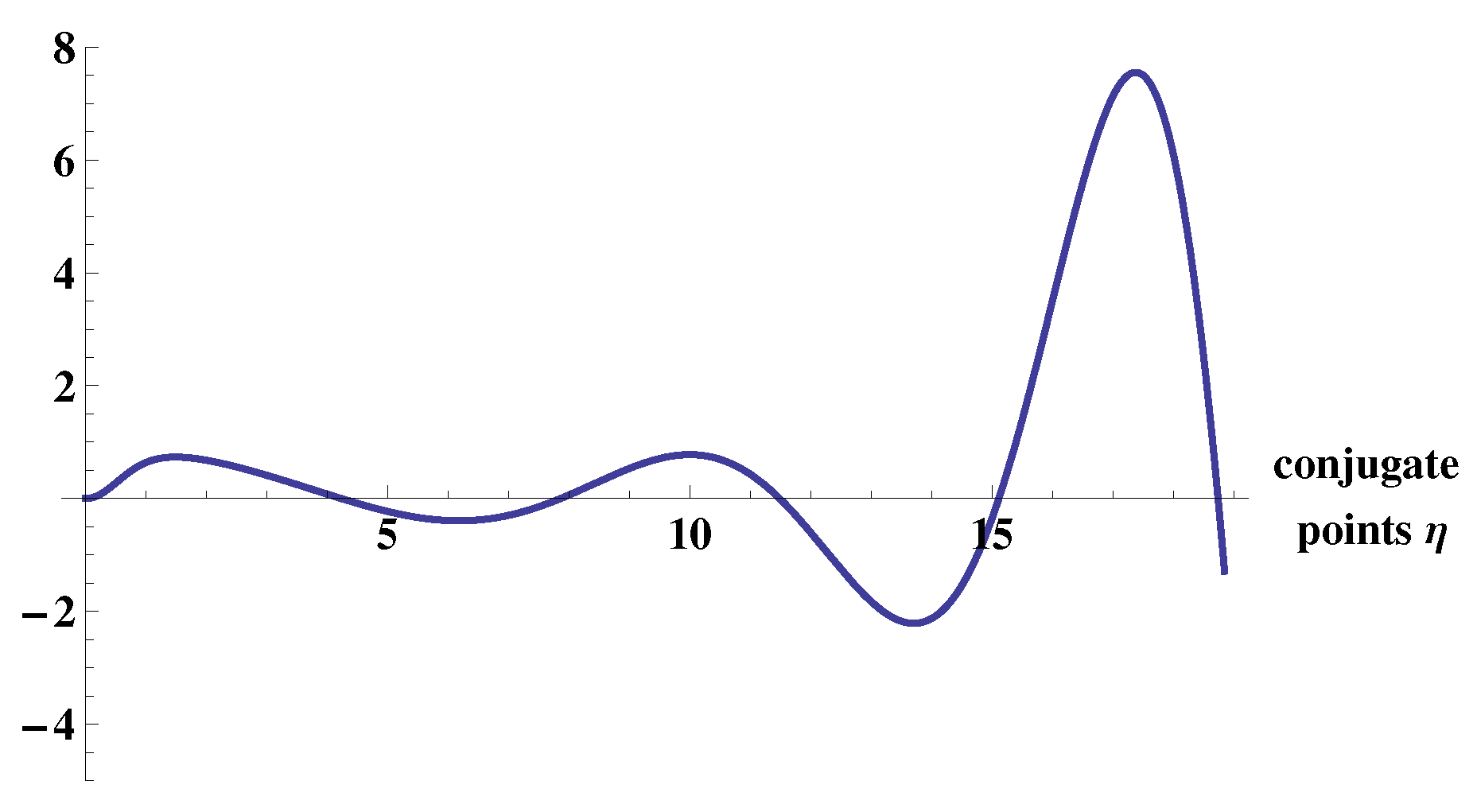
This system can have nontrivial solutions $C_2$ and $C_3$ only if the coefficient determinant is zero. Therefore we get the equation to find the conjugate (to $t=0$) points ${\eta }_k$

$$\frac{\sqrt{3}}{2}{e}^{-\eta }+\frac{3}{2}{e}^{\eta /2}sin\frac{\sqrt{3}}{2}\eta -\frac{\sqrt{3}}{2}{e}^{\eta /2}cos\frac{\sqrt{3}}{2}\eta =0$$

(11)

The graph (appropriately scaled to fit the area) of the function on the left side is depicted in Figure 1.

Conjugate points to $t=0$ of equation $x^{‴}=x$ coincide with conjugate points to $t=0$ of the adjoint equation $y^{‴}=-y.$ The conjugate points ${\xi }_k$ of the equation $y^{‴}=-y$ are exactly the zeros (all of them are simple zeros) of a solution $y\left(t\right)$ that satisfies the initial conditions $y\left(0\right)=y^{\prime }\left(0\right)=0.$

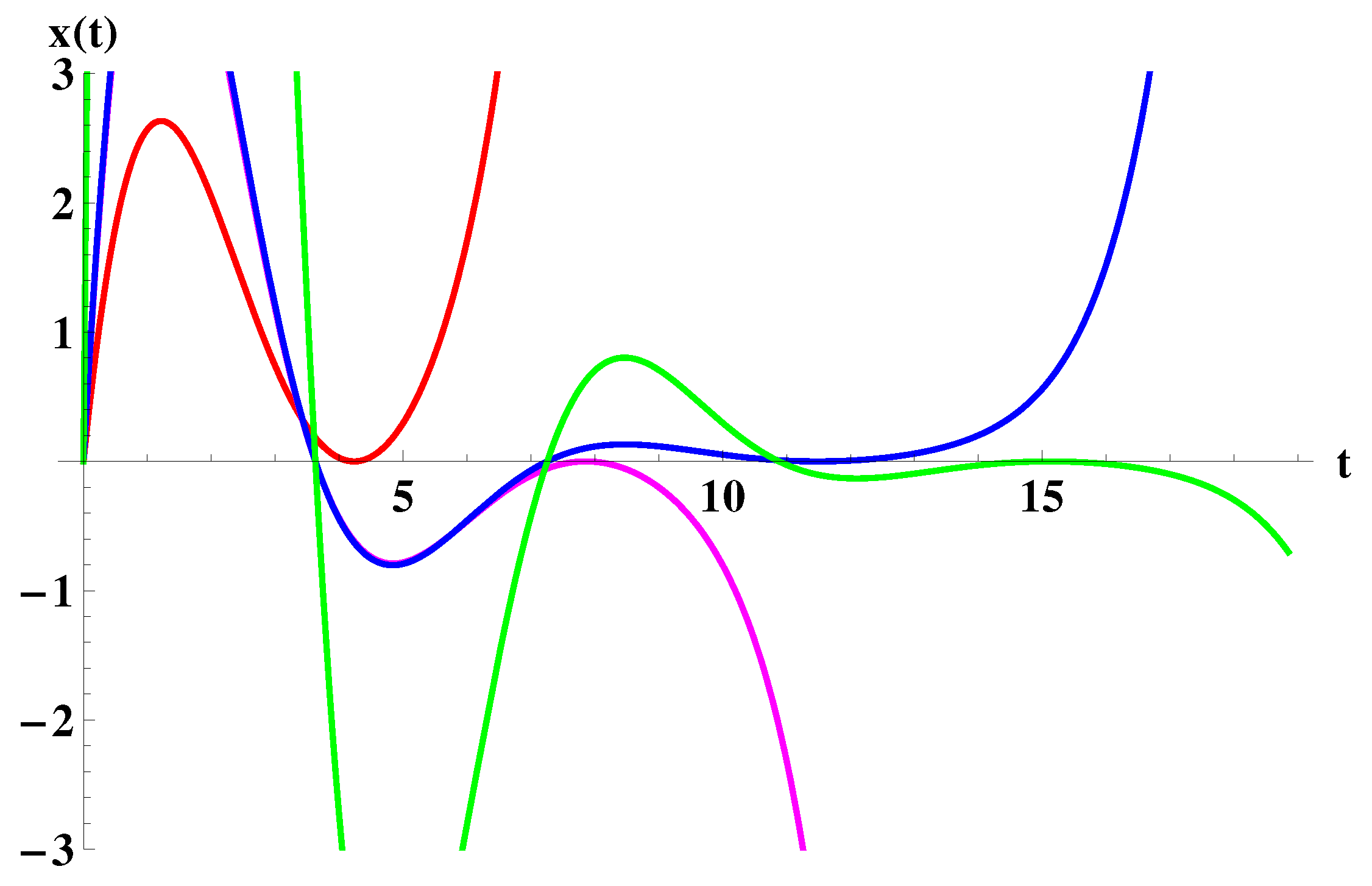
First four extremal solutions (with respect to $t=0$) for Equation (9) are depicted in Figure 2.

The angles ${\varphi }_k=arctan\frac{x_k^{″}\left(0\right)}{x_k^{\prime }\left(0\right)}$ that define the initial values for extremal solutions $x_k\left(t\right)$ are arranged

$$-\pi /2<{\varphi }_2<{\varphi }_4<\dots <{\varphi }_{2i}<\dots <{\varphi }_{2i+1}<\dots <{\varphi }_3<{\varphi }_1<0.$$

(12)

The respective extremal solutions $x_k\left(t\right)$ are defined then as

$$x_k\left(t\right)=\frac{tan{\varphi }_k+1}{3}{e}^t+e^{-\frac{1}{2}t}\left(\frac{1-tan{\varphi }_k}{\sqrt{3}}sin\frac{\sqrt{3}}{2}t-\frac{1+tan{\varphi }_k}{3}cos\frac{\sqrt{3}}{2}t\right)$$

(13)

The extremal solutions expressed in terms of conjugate points $\eta$

$$x\left(t\right)=e^{-\frac{1}{2}\eta }sin\frac{\sqrt{3}}{2}\eta \left(e^t-e^{-\frac{1}{2}t}cos\frac{\sqrt{3}}{2}t\right)+\left(e^{-\frac{1}{2}t}cos\frac{\sqrt{3}}{2}\eta -e^{\eta }\right)e^{-\frac{1}{2}t}sin\frac{\sqrt{3}}{2}t$$

(14)

Below the $tan{\varphi }_k$ are given (rounded to 12 digits) for the first six extremal solutions

$$\begin{array}{cc}\hfill tan{\varphi }_1=-0.9969785430602899;& tan{\varphi }_2=-1.0000131330764497;\hfill \\ \hfill tan{\varphi }_3=-0.9999999430896078;& tan{\varphi }_4=-1.0000000002466165;\hfill \\ \hfill tan{\varphi }_5=-0.9999999999989313;& tan{\varphi }_6=-1.0000000000000047.\hfill \end{array}$$

The sequences $\left\{{\varphi }_{2i}\right\}$ and $\left\{{\varphi }_{2i+1}\right\}$ tend from below and from above respectively to the angle ${\varphi }_{*}=-\frac{\pi }{4}.$ The particular solution defined by the angle ${\varphi }_{*}$ is

$$x_{*}\left(t\right)=\frac{2}{\sqrt{3}}{e}^{-\frac{1}{2}t}sin\frac{\sqrt{3}}{2}t.$$

(15)

This is oscillatory solution with equidistant zeros.

The convergence ${\varphi }_i\to -\frac{\pi }{4}$ is rapid and therefore the extremal solutions are hardly detectable numerically.

3. Phase Plane for Linear Equations

In order to visualize extremal solutions consider the variable change [15]

$$u_1=x^{\prime }{x}^{-1},u_2=x^{″}{x}^{-1},$$

which acts on intervals where $x\left(t\right)\ne 0.$ After standard calculations one arrives at the system

$$\left\{\begin{array}{cc}\hfill u_1^{\prime }& =u_2-u_1^2,\hfill \\ \hfill u_2^{\prime }& =1-u_1{u}_2.\hfill \end{array}\right.$$

(16)

The phase portrait for this system is depicted in Figure 3.

4. Emden Fowler Type Equations

Consider equations of the type

$$x^{‴}=p{\left|x\right|}^{\gamma }x,p>0,$$

(17)

for $\gamma >0.$ These equations exhibit generally the same behavior as the linear one with the exception that all solutions that eventually tend to infinity $x\left(t\right)\to \infty$ do so in finite time.

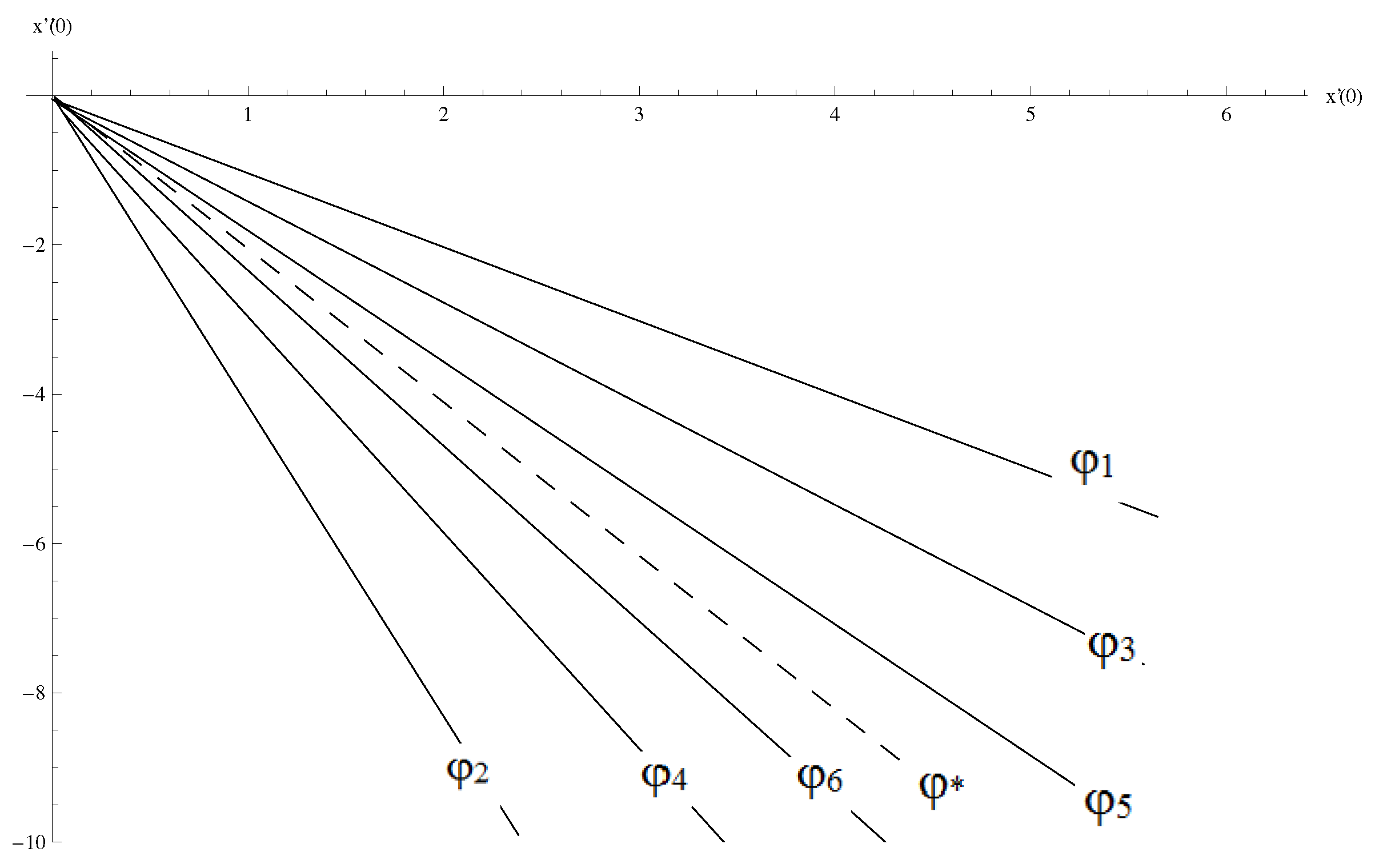
It can be proved that the plane of the initial data $(x^{\prime }\left(a\right),x^{″}\left(a\right))$ looks generally as that for the linear case (Figure 4).

Instead of straight lines defined by angles ${\varphi }_k$ in Figure 4 there are curves ${\Gamma }_k$ that are still arranged in two sequences converging to a specific branch ${\Gamma }_{*}.$ This branch contains the initial data (namely, $x^{\prime }\left(a\right)$ and $x^{″}\left(a\right)$) for extendable and oscillatory solutions that have not double zeros.

Generally, the following is true for solutions of (17) that vanish at $t=a.$ There exists a one-dimensional branch of the initial conditions ${\Gamma }_1$ that extends to the 4-th quadrant of the $(x^{\prime }\left(a\right),x^{″}\left(a\right))$-plane ($x^{\prime }\left(a\right)>0,$$x^{″}\left(a\right)<0$) and possesses the property: any solution of

$$x^{‴}=p{\left|x\right|}^{\gamma }x,x\left(a\right)=0,(x^{\prime }\left(a\right),x^{″}\left(a\right))\in {\Gamma }_1$$

(18)

is positive in the interval $(a,{\eta }_1)$, has a double zero at ${\eta }_1$ and is positive for $t>{\eta }_1.$ In the case of a linear equation ($\gamma =0$ in (17)) this branch is the straight line marked as ${\varphi }_1$ in Figure 4. Similar suggestions can be stated for other branches.

Lemma 1. 

Any solution of an Equation (17) with the initial conditions

$$x\left(a\right)=0,x^{\prime }\left(a\right)\ge 0,x^{″}\left(a\right)\ge 0,x^{\prime 2}\left(a\right)+x^{″2}\left(a\right)>0$$

(19)

remains positive for $t>a.$

Similarly, any solution with the conditions

$$x\left(a\right)=0,x^{\prime }\left(a\right)\le 0,x^{″}\left(a\right)\le 0,x^{\prime 2}\left(a\right)+x^{″2}\left(a\right)>0$$

(20)

remains negative for $t>a.$

Proof. 

Let (19) hold. Then one of the values $x^{\prime }\left(a\right)$ or $x^{″}\left(a\right)$ is positive and $x\left(t\right)$ is positive also in some right neighborhood $(a,b)$ of the point $t=a.$ Suppose $x\left(b\right)=0.$ Then $x^{\prime }\left(b_1\right)=0$ for some $b_1\in (a,b)$ and $x^{″}\left(b_2\right)<0$ for some $b_2\in (a,b_1).$ This is impossible, however, since $x^{″}\left(a\right)\ge 0$ and $x^{‴}\left(t\right)>0$ whenever $x\left(t\right)$ is positive, namely, $x^{‴}\left(t\right)>0$ for $t\in (a,b).$

Similarly $x\left(t\right)<0$ for $t>a$ if (20) holds. □

Lemma 2. 

Let x and y be solutions of an Equation (17) with the initial conditions

$$x\left(a\right)=y\left(a\right),x^{\prime }\left(a\right)=y^{\prime }\left(a\right),x^{″}\left(a\right)>y^{″}\left(a\right).$$

(21)

Then $x\left(t\right)>y\left(t\right)$ for $t>a.$

Proof. 

Write (17) as $x^{‴}=pf\left(x\right),$ where $f\left(x\right)={\left|x\right|}^{\gamma }x.$ Notice that $f^{\prime }\left(x\right)>0$ for $x\ne 0.$ Consider the difference $u\left(t\right)=x\left(t\right)-y\left(t\right).$ One has that

$$u^{‴}=p(f\left(x\left(t\right)\right)-f\left(y\left(t\right)\right)=p{f}^{\prime }\left(\theta \left(t\right)\right)(x\left(t\right)-y\left(t\right)=p{f}^{\prime }\left(\theta \left(t\right)\right)u,$$

(22)

where $\theta$ is some intermediate value. The function $u\left(t\right)$ satisfies $u\left(a\right)=0,$ $u^{\prime }\left(a\right)=0,$ $u^{″}\left(a\right)>0.$ Since linear Equation (22) is of Class II (recall that $p{f}^{\prime }\left(\theta \left(t\right)\right)>0$), $u\left(t\right)>0$ for $t>a$ as long as both solutions exist. Hence the proof. □

Consider Equation (17) with $p=const>0$ and $\gamma >0.$

Theorem 3. 

For any $t=a$ there exist branches ${\Gamma }_i$ ($i=1,2,\dots$) of the initial values $(x^{\prime }\left(a\right),x^{″}\left(a\right))$ possessing the properties:

(1) ${\Gamma }_i$ locate in the quadrant $(x^{\prime }>0,x^{″}<0)$ of the $(x^{\prime }\left(a\right),x^{″}\left(a\right))$-plane;

(2) ${\Gamma }_i$ emanate from the origin $(0,0)$ and extend to infinity;

(3) ${\Gamma }_i$ are ordered as

$${\Gamma }_2\prec {\Gamma }_4\prec \dots \prec {\Gamma }_{2i}\prec \dots \prec {\Gamma }_{2j+1}\prec \dots \prec {\Gamma }_3\prec {\Gamma }_1$$

in the meaning that any vertical line $x^{\prime }=const>0$ crosses branches ${\Gamma }_i$ in indicated order;

(4) solutions $x_i\left(t\right)$ of Equation (17) subject to the initial conditions $x\left(a\right)=0,$$(x^{\prime }\left(a\right),x^{″}\left(a\right))\in {\Gamma }_{2i+1},$ ($i=0,1,\dots$) have exactly $i-1$ simple zeros in the interval $(a,\eta )$ and a double zero at $t=\eta$ (different η for different x);

(5) solutions $x_i\left(t\right)$ of Equation (17) subject to the initial conditions $x\left(a\right)=0,$$(x^{\prime }\left(a\right),x^{″}\left(a\right))\in {\Gamma }_{2i},$ ($i=1,\dots$) have exactly i simple zeros in the interval $(a,\eta )$ and a double zero at $t=\eta$ (different η for different x);

(6) solutions $x\left(t\right),$ defined by the initial conditions

$$x\left(a\right)=0,{\Gamma }_{2i}\prec (x^{\prime }\left(a\right),x^{″}\left(a\right))\prec {\Gamma }_{2i+2},$$

have for $t>a$ exactly $2i+2$ simple zeros, and solutions defined by the initial conditions

$$x\left(a\right)=0,{\Gamma }_{2i+1}\prec (x^{\prime }\left(a\right),x^{″}\left(a\right))\prec {\Gamma }_{2i-1},i=0,1,2,\dots$$

have for $t>a$ exactly $2i+1$ simple zeros (${\Gamma }_0$ means semi-axis $(x^{\prime }\left(a\right)=0,x^{″}\left(a\right)<0)$ and ${\Gamma }_{-1}$ means $(x^{\prime }\left(a\right)>0,x^{″}\left(a\right)=0)$).

Proof. 

Fix $R>0$ and consider a quarter of a circle of radius R in the $(x^{\prime }\left(a\right),x^{″}\left(a\right))$-plane lying in the 4-th quadrant ($x^{\prime }>0,$ $x^{″}<0$). Parameterize the arc by the angle $\varphi =arctan\frac{x^{″}\left(a\right)}{x^{\prime }\left(a\right)}$ that takes values in the interval $[0,-\frac{\pi }{2}].$ Due to Lemma 1 a solution with the initial conditions $x\left(a\right)=0,$$x^{\prime }\left(a\right)=R,$$x^{″}\left(a\right)=0$ or, equivalently $\phi =0,$ is positive for $t>a.$ A solution with the initial conditions $x\left(a\right)=0,$$x^{\prime }\left(a\right)=0,$$x^{″}\left(a\right)=-R$ or, equivalently $\phi =-\frac{\pi }{2},$ is negative for $t>a$.

Denote solutions of Equation (17) satisfying the initial conditions $x\left(a\right)=0,$$x^{\prime 2}\left(a\right)+x^{″2}\left(a\right)=R^2,$$x^{\prime }\left(a\right)>0,$$x^{″}\left(a\right)<0$ by $x(t;\phi ).$ Solutions $x(t;\phi )$ continuously change together with $\phi .$

Let $\phi$ decrease from zero. For small (in modulus) $\phi$ solutions $x(t;\phi )$ are positive for $t>a.$ Let ${\phi }_1=inf\{\phi \in (-\pi /2,0):x\left(t\right)>0 \mathrm{f}\mathrm{o}\mathrm{r} t>a\mathrm{i}\mathrm{n} \mathrm{t}\mathrm{h}\mathrm{e} \mathrm{i}\mathrm{n}\mathrm{t}\mathrm{e}\mathrm{r}\mathrm{v}\mathrm{a}\mathrm{l} \mathrm{o}\mathrm{f} \mathrm{d}\mathrm{e}\mathrm{f}\mathrm{i}\mathrm{n}\mathrm{i}\mathrm{t}\mathrm{i}\mathrm{o}\mathrm{n}\}.$ Such a value exists since solutions $x(t;\phi )$ for $\phi \to -\pi /2$ are negative. A solution $x(t;{\phi }_1)$ has a zero, otherwise it is positive in the interval of definition. This zero (denote it ${\eta }_1\left(R\right)$) must be double zero ($x=0,$$x^{\prime }=0$). If it is simple ($x^{\prime }\ne 0$) then there exists some $\phi >{\phi }_1$ with the same extremal property and this contradicts the definition of ${\phi }_1.$ Next solutions with $\phi$ less than ${\phi }_1$ but close to it can be considered. They have simple zeros $t_1<{\eta }_1<t_2$ (by Lemma 2) and are positive for $t>t_2.$ The lower bound of $\phi$ for solutions with this property yields ${\eta }_3\left(R\right).$ Proceeding in this way we can obtain ${\eta }_{2i+1}$ for any number i.

Considering solutions $x(t;\phi )$ starting from $\phi =-\pi /2$ we obtain solutions with a double zero at ${\eta }_2,$${\eta }_4$ and so on. These solutions are negative eventually. For instance, set ${\phi }_2=sup\{\phi \in (-\pi /2,0):\exists \tau >a\mathrm{s}\mathrm{u}\mathrm{c}\mathrm{h} \mathrm{t}\mathrm{h}\mathrm{a}\mathrm{t} x\left(t\right)>0 \mathrm{f}\mathrm{o}\mathrm{r} \tau >t>a,x\left(t\right)<0 \mathrm{f}\mathrm{o}\mathrm{r} t>\tau \mathrm{i}\mathrm{n} \mathrm{t}\mathrm{h}\mathrm{e} \mathrm{i}\mathrm{n}\mathrm{t}\mathrm{e}\mathrm{r}\mathrm{v}\mathrm{a}\mathrm{l} \mathrm{o}\mathrm{f} \mathrm{d}\mathrm{e}\mathrm{f}\mathrm{i}\mathrm{n}\mathrm{i}\mathrm{t}\mathrm{i}\mathrm{o}\mathrm{n}\}.$ A solution $x(t;{\phi }_2)$ has a zero at some point ${\eta }_2\left(R\right)>\tau .$ This zero must be double one, due to the extremal property (simple zero is not allowed).

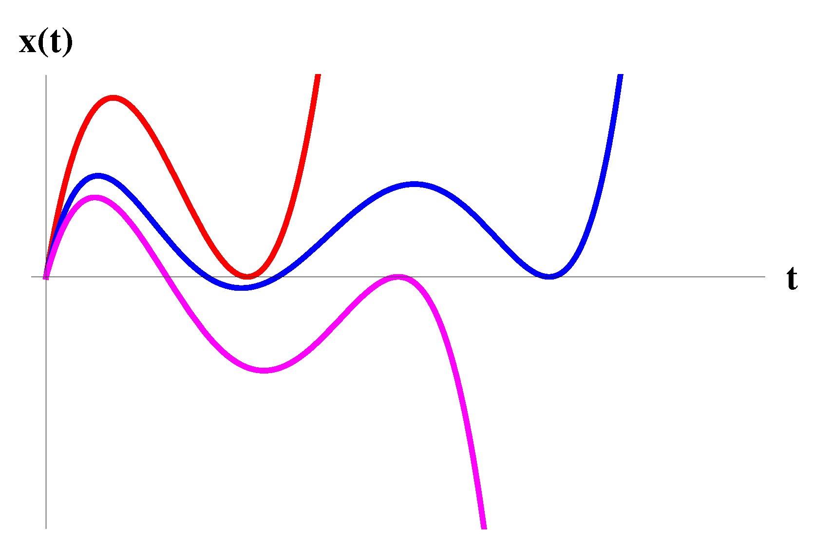
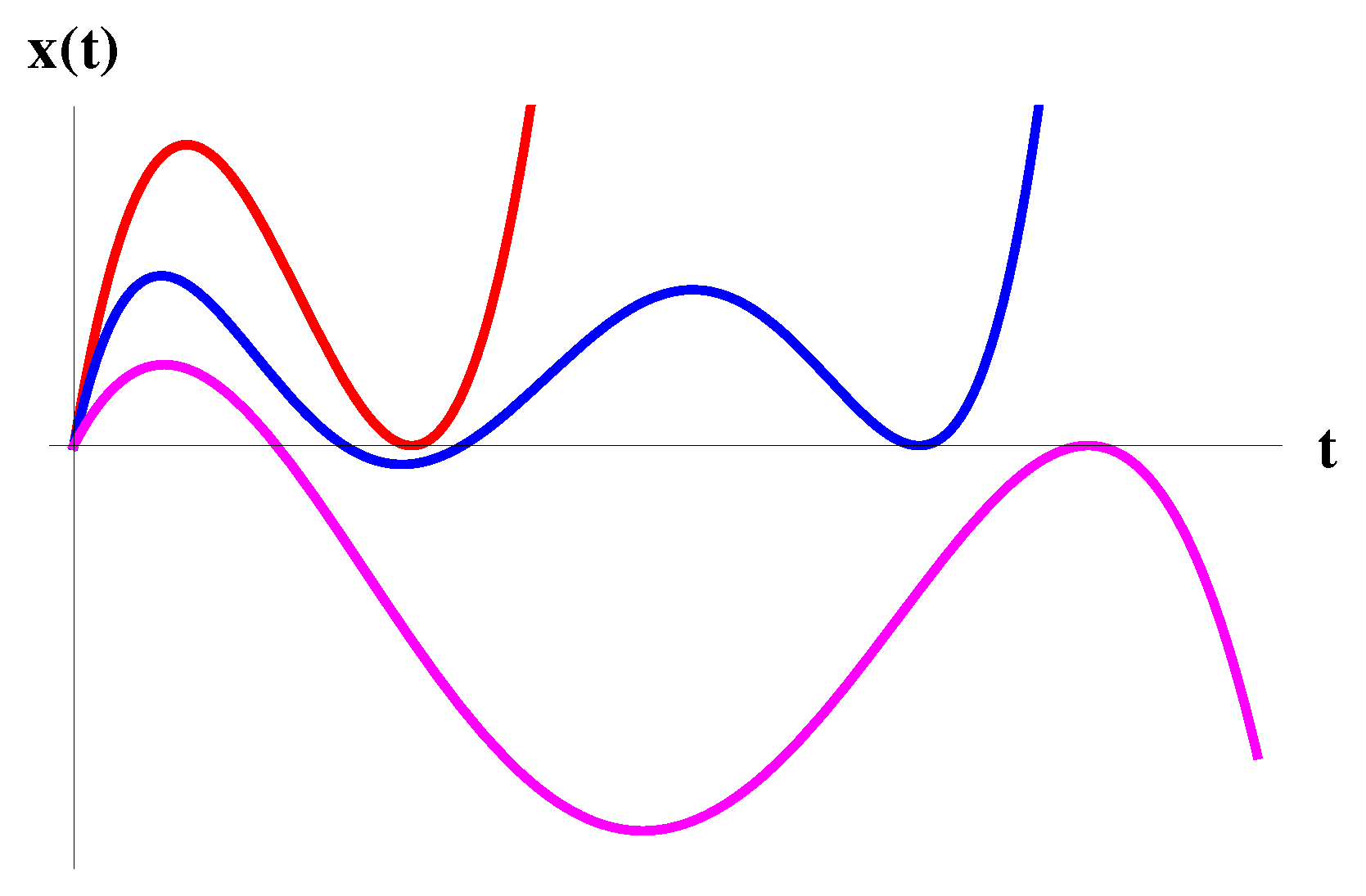
By construction,

$${\eta }_1<{\eta }_3<\dots <{\eta }_{odd}<\dots$$

and, similarly,

$${\eta }_2<{\eta }_4<\dots <{\eta }_{even}<\dots$$

It can be shown that odd and even $\eta$ alternate. Look at Figure 5, Figure 6 and Figure 7. If solutions $x(t;{\phi }_1),$ $x(t;{\phi }_2)$ and $x(t;{\phi }_3)$ with $0>{\phi }_1>{\phi }_2>{\phi }_3>-\pi /2$ behave like in Figure 5 then “between” “blue” and “magenta” solutions there exists a solution with the first double zero $\xi <{\eta }_1.$ This contradicts the choice of ${\eta }_1$ as the first double zero. The only possible location of $\eta$-s is as in Figure 6. The arrangement of solutions as in Figure 7 is not valid also. □

5. More on Nonlinear Equations

Solutions of equations of the form

$$x^{‴}=p{\left|x\right|}^{\gamma }x,$$

(23)

where continuous coefficient $p=p\left(t\right)>0$ and $\gamma >0$ possess the following properties.

Since we are looking for solutions of (23) that have double zero consider the case

$$x\left(a\right)=0,x^{\prime }\left(a\right)>0,x^{″}\left(a\right)<0.$$

(24)

The case

$$x\left(a\right)=0,x^{\prime }\left(a\right)<0,x^{″}\left(a\right)>0$$

(25)

is symmetric.

Due to Theorem 3 there are solutions with the initial values $x\left(a\right)=0,$$(x^{\prime }\left(a\right), x^{″}\left(a\right))\in {\Gamma }_1,$ which have a double zero at some point $\eta >a,$ and $x^{″}\left(\eta \right)>0.$ Then such a solution is positive for $t>\eta .$ Solutions with $x\left(a\right)=0$ and $(x^{\prime }\left(a\right),x^{″}\left(a\right))\in {\Gamma }_i$ also have a double zero at some point $\eta$ (individual for any solution) and do not change the sign for $t>\eta .$ For odd i these solutions are positive and for even i they are negative for $t>\eta .$ Therefore the following assertion is true.

Lemma 3. 

Let $0<p_{min}\le p\left(t\right)\le p_{max}.$ Then any solution with $x\left(a\right)=0,$ $x^{\prime }\left(a\right)>0$ which has a double zero at some point $\eta >a$ has the vertical asymptote.

Proof. 

Follows from Lemmas 4.2 and 4.3 in [15]. □

Suppose $x\left(t\right)$ is a solution of the Equation (23) with the initial conditions $x\left(0\right)=0,$$x^{\prime }\left(0\right)>0,$$x^{″}\left(0\right)<0$ and with a double zero at $t=\eta >0.$ For brevity, let us call such a solution extremal solution. In contrast to the linear case, multiples of extremal solutions need not be an extremal one.

Let $p=const>0.$ Any extremal solution may oscillate, having several zeros in the interval $(0,\eta )$ and a double zero at $t=\eta .$ Then it is either eventually positive, or negative, like in Figure 8 and Figure 9. Due to Lemma 3, any such solution must have the vertical asymptote. The next statement, which is a consequence of Theorem 4.4 in [15], describes the asymptotics of extremal solutions.

Lemma 4. 

Any extremal solution has asymptotics $C{(t_{*}-t)}^{-\frac{\gamma }{3}}(1+o\left(1\right)),$ where

$$C={\left[\frac{\frac{3}{\gamma }(\frac{3}{\gamma }+1)(\frac{3}{\gamma }+2)}{p}\right]}^{\frac{3}{\gamma }}$$

(26)

and $t=t_{*}$ is the vertical asymptote for a solution.

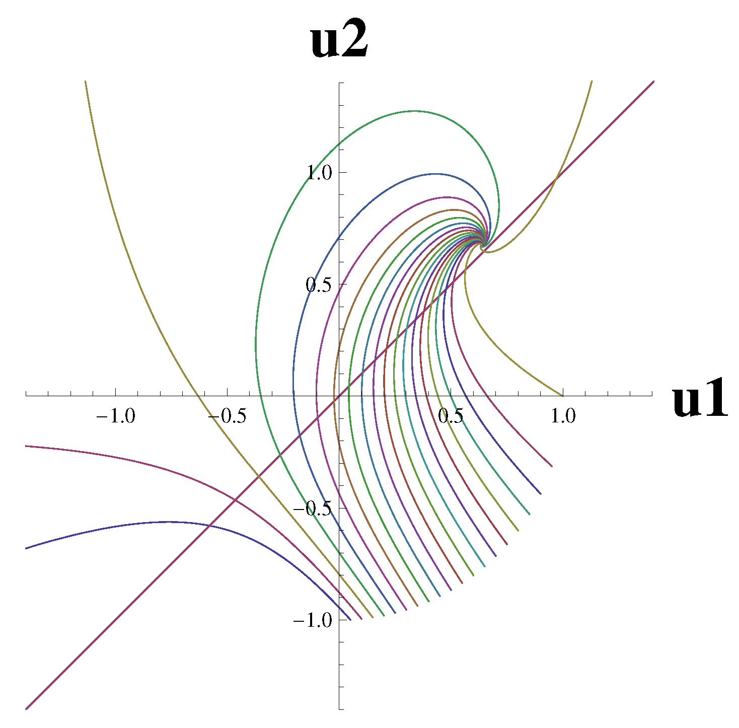
There is another description of the asymptotic behavior of extremal solutions. Let us, following [15] (§4.3), introduce new functions

$$u_1\left(t\right)=\frac{x^{\prime }\left(t\right)}{x^{{\beta }_1}},u_2\left(t\right)=\frac{x^{″}\left(t\right)}{x^{{\beta }_2}},where{\beta }_1=1+\frac{\gamma }{3},{\beta }_2=1+\frac{2\gamma }{3}.$$

By standard differentiation of $u_i\left(t\right)$ with respect to t and taking into account (17) we can obtain a two-dimensional non-autonomous system of differential equations. Continue with introduction the independent variable $z={\int }_{\eta }^t{x}^{\frac{\gamma }{3}}\left(s\right)ds$ for any extremal solution $x\left(t\right).$ In view of Lemmas 3 and 4, $z\to +\infty$ as $t\to t_{*},$ where $t=t_{*}$ is an asymptote for $x\left(t\right).$ Functions $u_i,$ considered as functions of the variable $z,$ satisfy the autonomous system

$$\left\{\begin{array}{c}{u}_1^{\prime }=u_2-\frac{3+\gamma }{3}{u}_1^2,\\ u_2^{\prime }=p-\frac{3+2\gamma }{3}{u}_1{u}_2\end{array}\right.$$

(27)

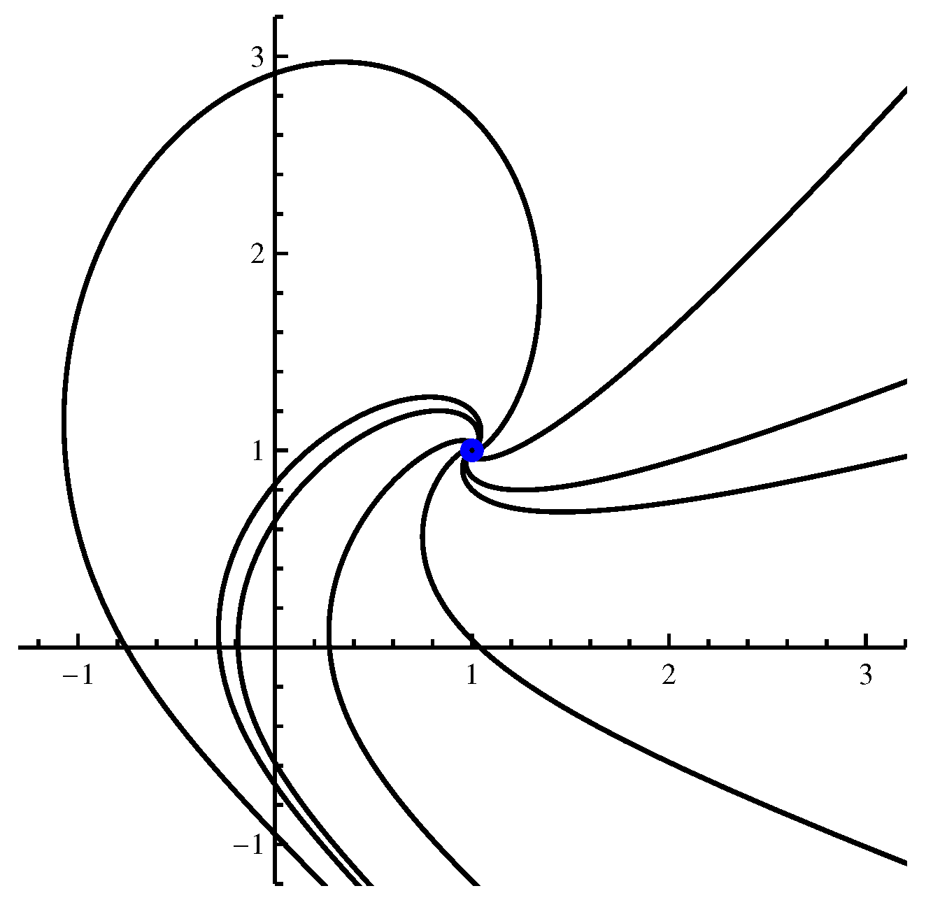
Any extremal solution $x\left(t\right)$ generates a phase trajectory $(u_1\left(z\right),u_2\left(z\right)),$ which tends to a single critical point of (27). The phase portrait for (27) is depicted in Figure 10.

6. Conclusions

The structure of a set of extremal solutions, associated with the conjugate points accordingly to the linear theory by M. Hanan [2], is revealed. There are two groups of extremal solutions. Solutions of the first group, after several oscillations, go to $+\infty .$ Solutions of the second group go to $-\infty .$ Their initial conditions become extremely close, so they are very difficult to discover numerically. Both groups are separated by a solution with an infinite number of zeros. This solution for $p=const$ in the Equation (1) is unique.

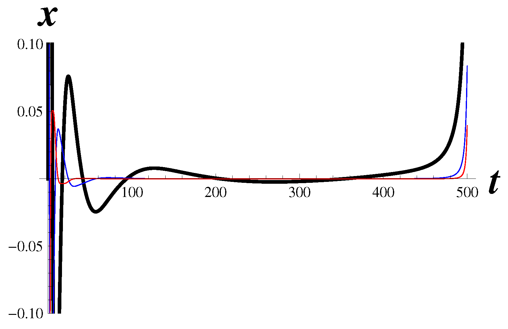
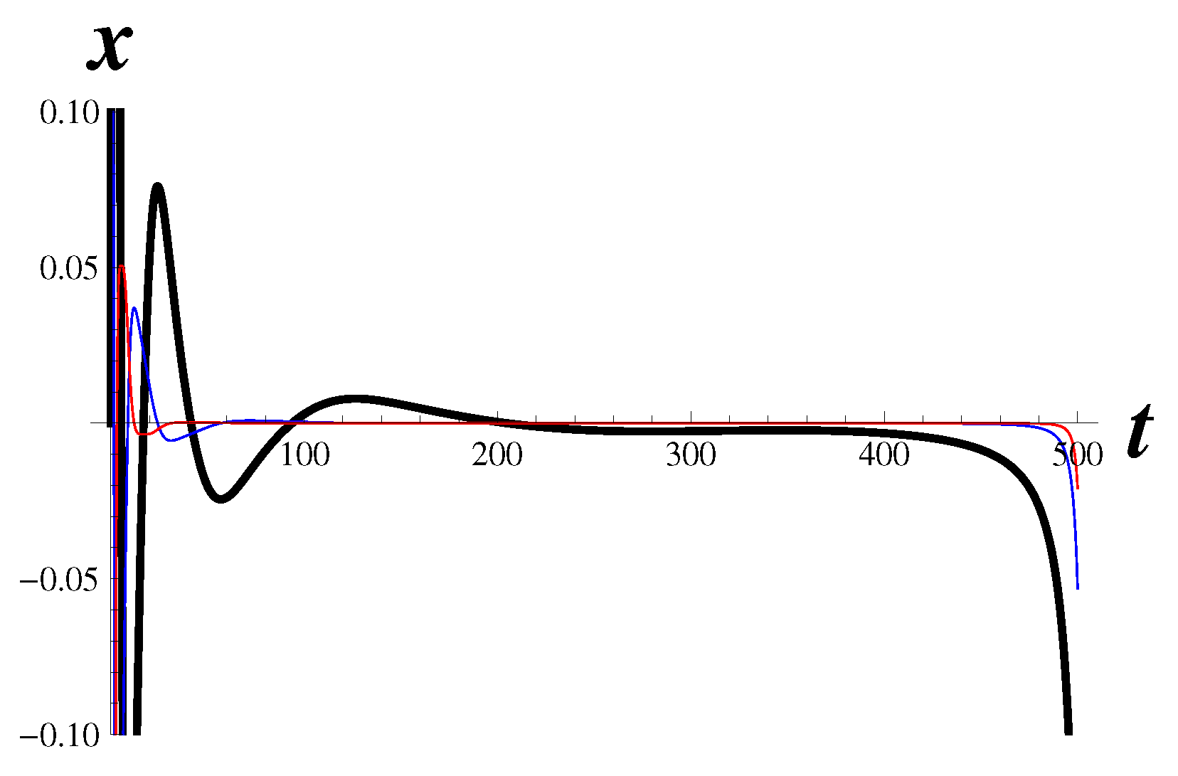
For nonlinear equations of the Emden-Fowler type, the structure of a set of solutions, satisfying the initial conditions $x\left(0\right)=0,$ $x^{\prime }\left(0\right)>0,$$x^{″}\left(0\right)<0,$ and having a double zero to the right of $t=0,$ is similar to that of linear equations. There are no conjugate points, however. To find numerically the initial conditions for a solution, which has a double zero at some prescribed point, can be a difficult task. Solutions of nonlinear equations also form two groups. Solutions of both groups end respectively at $+\infty ,$ or at $-\infty .$ Both groups are separated by an oscillatory solution (-ns), which is hard to find. In the two below pictures the graphs of two solutions to the equation $x^{‴}={\left|x\right|}^{2}x$ are depicted.

They belong to different groups, their behavior is essentially different, but the initial conditions for the second derivative differ only after 22 decimal places.

When looking for solutions of a certain structure (for example, solutions with a given number of zeros), one must be careful, since even for formally simple ODE, they (solutions) can be overlooked when conducting numerical experiments. This applies to ODEs already of the third order and higher. Data on the mutual arrangement of solutions can be used in the study of multiple solutions of boundary value problems [16,17].