Article

Validation of Replicable Pipeline 3D Surface Reconstruction for Patient-Specific Abdominal Aortic Lumen Diagnostics

1
Department of Industrial Engineering (DIN), Università di Bologna, 40136 Bologna, Italy
2
Independent Researcher, 40128 Bologna, Italy
3
Division of Vascular Surgery, Alessandro Manzoni Hospital, 23900 Lecco, Italy
4
Department of Computer Science—Science and Engineering, University of Bologna, 40126 Bologna, Italy
5
Vascular Surgery, Department of Medical and Surgical Sciences, University of Bologna, 40138 Bologna, Italy
6
Vascular Surgery Unit, IRCCS S. Orsola Hospital, 40138 Bologna, Italy
*
Author to whom correspondence should be addressed.
Submission received: 11 February 2025 / Revised: 17 March 2025 / Accepted: 18 March 2025 / Published: 25 March 2025
(This article belongs to the Topic Machine Learning and Deep Learning in Medical Imaging)

Abstract

:
Background: Accurate prognoses are challenging in high-risk vascular conditions, such as abdominal aortic aneurysms, and limited diagnostic standards, decision-making criteria, and data semantics often hinder clinical reliability and impede diagnostics’ digital transition. This study aims to evaluate the performance, robustness, and usability of an automatic, replicable pipeline for aortic lumen surface reconstruction for pathological vessels. The goal is to provide a solid tool for geometric reconstruction to a more complex enhanced diagnostic framework. Methods: A U-Net convolutional neural network is trained using preoperative CTA scans, with 101 for model training and 14 for model testing, covering a wide anatomical and aortoiliac pathology spectrum. Validation included segmentation metric, robustness, reliability, and usability assessments. Performances are investigated by means of the test set’s prediction metrics for several instances of the model’s input. Clinical reliability is evaluated based on manual measurements performed by a vascular surgeon on the obtained 3D aortic lumen surfaces. Results: The test set is selected to cover a wide portion of aortoiliac pathologies. The algorithm demonstrated robustness with an average F1-score of 0.850 ± 0.120 and an intersection over union score of 0.760 ± 0.150 in the test set. Clinical reliability is assessed using the mean absolute errors for diameter and length measurements, respectively, of 1.73 mm and 2.27 mm. The 3D surface reconstruction demonstrated reliability, low processing times, and clinically valid reconstructions. Conclusions: The proposed algorithm can correctly reconstruct pathological vessels. Secondary aortoiliac pathologies are detected properly for challenging anatomies. To conclude, the proposed 3D reconstruction application to a digital, patient-specific diagnostic tool is, therefore, possible. Automatic replicable pipelines ensured the usability of the model’s outputs.

Graphical Abstract

1. Introduction

An AAA is an enlargement of the abdominal aorta, such that the diameter is more than 3 cm or 50% larger than its healthy, baseline value. Accurate monitoring, diagnostics, and timely intervention are crucial for preventing the high morbidity and mortality rates associated with such pathology. EVAR treatment represents the gold standard when the aortic anatomy is feasible, and its planning is, in fact, fundamental for technical success and endograft durability.
The cardiovascular community has proposed guidelines to streamline the surgery decision-making process and planning of abdominal aortic aneurysms. One such approach, proposed by Ouriel et al. [1], is based on a threshold-based method using maximum diameter measurements. The suggested threshold values are 55 mm for men and 50 mm for women. However, this approach has proven to be unreliable in predicting abdominal aortic aneurysm ruptures, as indicated by subsequent studies. In fact, Finol et al. [2] showed how the rupture risk does not linearly depend on the maximum diameter. To improve decision-making criteria, El Chaikoff et al. [3] introduced more complex methods for rupture risk assessment, moving beyond purely geometrical, threshold-based approaches. Additionally, Parkinson et al. [4] demonstrated that the rupture rate for abdominal aortic aneurysms ranging from 40 mm to 49 mm, though low, was still significant. Similarly, Darling et al. [5] reported that 23% of abdominal aortic aneurysms ruptured at sizes under 50 mm. Over the past decade, DL techniques have been vastly employed in the semantic segmentation of the aortic lumen in EVAR planning. Lately, Fantazzini et al. [6] have contributed to the segmentation task by training single- and multi-view U-Net models for aortic lumen semantic segmentation on 70 CTAs. However, the need for more widely distributed datasets is crucial, as the network is trained on a limited spectrum of abdominal aortic aneurysm anatomical features. An extension of previous work by the same research group proposed a novel model for the automatic segmentation and geometrical analysis of abdominal aortic aneurysms, along with the identification of intraluminal thrombus presence, as presented in Brutti et al. [7]. The model’s clinical validation involved a comparison between network measurements and those made by expert users. In another study by Adam et al. [8], fully automated routine presurgical measurements of the axial aortic lumen and outer-to-outer aortic wall diameter for endovascular aortic repair were proposed. The authors trained a V-Net [9] in large datasets consisting of 489 and 62 CTA sets for training and testing, respectively. The results showed mean Dice–Sørensen coefficients of 0.95 for diseased abdominal aortas and 0.84 for healthy aortas, indicating reliable performance. However, both studies acknowledged the necessity of including vastly different abdominal aortic aneurysm topologies in the training and validation sets to improve the model’s consistency and stability. Lastly, Lopez-Linares et al. [10] similarly proposed a work in which a fully automatic segmentation pipeline is adopted for a thrombus and an aortic lumen for postoperative CTAs. A convolutional neural network was trained on postoperative CTA images to automatically segment the aortic lumen and thrombus after EVAR. The absence of any required input makes the model very suitable for the interoperability and replicability of the results. A mean Dice–Sørensen coefficient of 0.83 is obtained. Although the results fit with the ones provided by the state of the art, such an approach does not clinically validate the model. Aortic measurements are, in fact, crucial to assessing how well the network does approximate 3D surface reconstruction.
The purpose of this study is to validate a 3D reconstruction methodology for the abdominal aortic vessel. Its application will not be solely limited to EVAR planning; it also serves as an initial step in the development of an automatic patient-specific CFD workflow with the goal of future works aiming to assess the aortic wall’s rupture risk. This first step is to obtain an anatomically accurate 3D model of the reconstructed aorta. By addressing the segmentation performance, robustness, and clinical reliability of the pipeline on several anatomies, the model’s usability and clinical consistency are assessed. The employment of such a mono-input 3D surface generation algorithm in complex hemodynamic solvers will enhance the quantitative CFD analysis of the aneurysmatic blood flow. To accomplish this, obtaining quality meshes is key in terms of the numerical stability and accuracy of the solution. The DL approach will help users in obtaining anatomically correct 3D models, which will be used for EVAR planning and patient-specific hemodynamic digital analysis.

2. Materials and Methods

2.1. Study Design

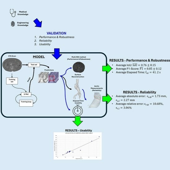
This study evaluates the performance, replicability and usability of a DL-based aortic lumen reconstruction and measurement pipeline, which is crucial when planning safety-critical tasks like abdominal aortic aneurysm EVAR. The goal is to develop and validate a robust single-class model that is capable of accurately detecting specific aorto-iliac anatomies. Four key characteristics—segmentation performance, robustness, reliability, and usability—are assessed based on [11,12].
Segmentation performances are evaluated by means of intersection over union and F1-score metrics; the former evaluates more accurately bad classification instances, and they, respectively, reflect the worst and average performance of the network among each test set anatomy.
Robustness is tested on input ROI translation along absolute and partial cardinal directions. By predicting multiple input instances, the network’s behavior is observed so as to assess segmentation metrics sensitivity with respect to input perturbations.
Reliability is validated by comparing manual measurements, performed by a vascular surgeon, on 3D reconstructions computed by the model, together with the ones obtained with reference software. Usability is evaluated based on input requirements and elapsed time.
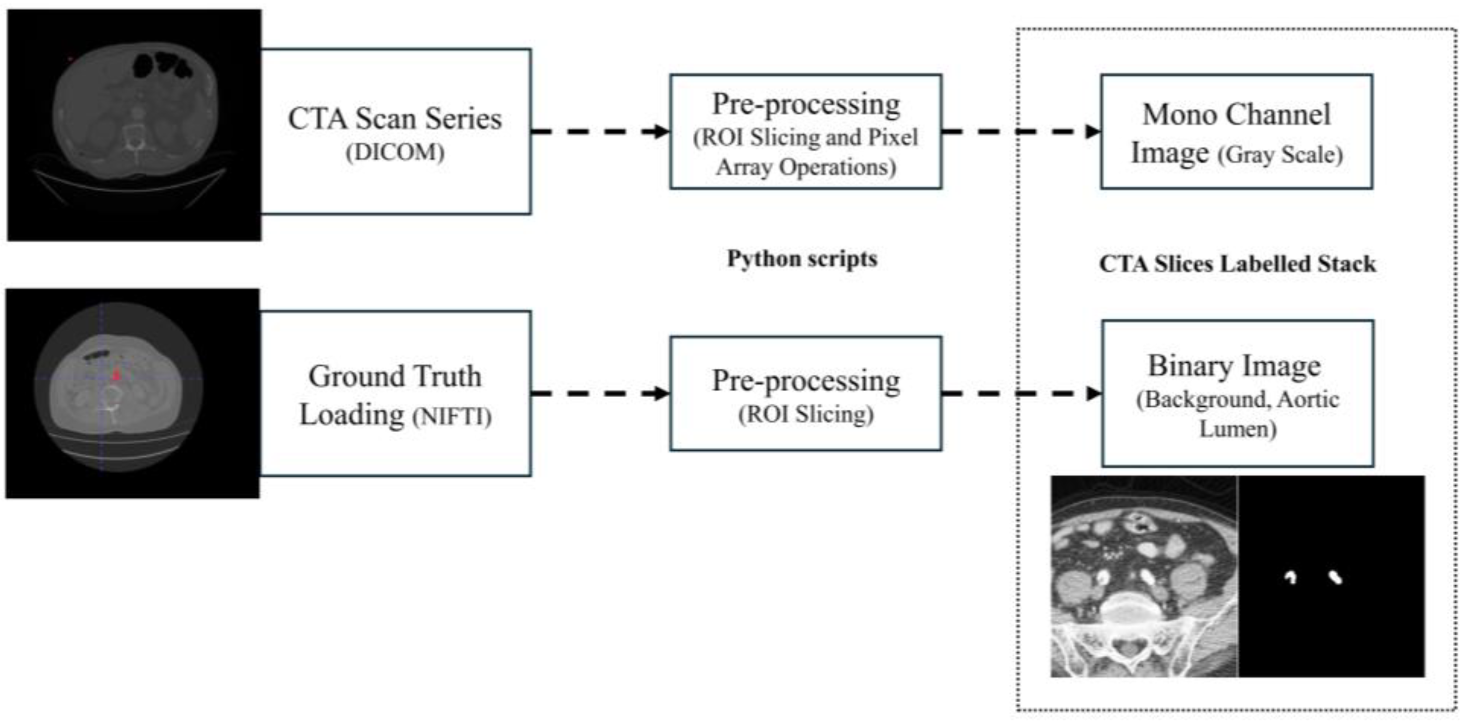
The methodology workflow is schematized in Figure 1. From the original CTA image and its relative mask, the original–GT image couples are extracted by a Python (v. 3.11.6) script. Masks and GT are obtained from widely known reference software ITK-Snap, (v. 4.0.2) [13] (ITK-SNAP Home, itksnap.org). Once the dataset is built, the network is trained. At testing time, the raw prediction’s output stack is processed to obtain the reconstructed aortic lumen’s surface and test metrics, following the performance, robustness, reliability, and usability assessments cited above.
Several tools are exploited by the model and the evaluation algorithm. Images are semi-automatically processed with ITK-Snap and Python [14]. The network is implemented using the Pytorch framework. Centerlines are obtained with the VMTK [15] toolkit. Measurements are performed manually on the widely known post-processing toolkit Paraview [16]. It must be underlined that all segmentations are performed exclusively using a CPU device to assess the algorithm performance in the most general usage context. The user is provided with a graphics user interface to perform CTA slicing, prediction, centerline extraction and 3D reconstructions.

2.2. Data Acquisition and GT Extraction

In this study, training, evaluation, and test data were provided by a single sanitary structure of the Lombardia region in anonymous form. The following diagnostic devices are used to collect imaging data: General Electric’s LightSpeed16 Rad (Cincinnati, OH, USA), Philip’s (Amsterdam, Netherlands) iCT SP, Ingenuity CT, and Brilliance 16. The spatial resolution ranges from 0.779 mm to 0.977 in the x and y directions. Axial slices are extracted by slicing the DICOM volume of interest. The data pool is composed of N C T s , t o t t r a i n e v a l = 101 , N C T s , t o t t e s t = 14 axial CTA and includes aneurysmatic patients with a mean age of 75.6 ± 7.67. The data pool consists of 114,141 images split into training, validation and testing with an 80%–15%–5% distribution.
GT extraction is performed using ITK-Snap’s thresholding semi-automatic active contouring and a custom Python script to generate input and target images. ITK-snap (v. 4.0.2) is the chosen reference labeling software for its wide consensus across the biomedical engineering community. The interest area includes the abdominal section, ranging from common iliac arteries to the celiac trunk. Upper and lower threshold values are selected to isolate CTA’s contrast medium in the abdominal aortic region. Usually, this process takes some parameter tuning, repeating the labeling multiple times. Despite this, its low characteristic operative time and simple active contouring based semi-automatic segmentation guarantee a reasonable amount of time effort by the trained personnel. The engineering team has been trained in the aortic lumen labeling task under the supervision of a vascular surgeon.
The Python script extracts the input CTA and GT, respectively, starting from the DICOM series pixel array and NIFTI (Neuroimaging Informatics Technology Initiative) GT array proxy files, the latter obtained from ITK-Snap labeling method. Then, images and GT volumes are cropped along the ROI. Finally, histogram equalization is applied to the original images. The output of the script is a stack of mono-channel gray CTA images and a stack of mono-channel binary GT images. The extraction algorithm is schematized in Figure 2. The target patient’s CTA and GT NIFTI file is loaded into the Python script following DICOM Series attributes [17], such as Image Position Patient, Pixel Spacing, Slice Thickness and Spacing Between Slices, to sort and extract angiography series. The algorithm now pre-processes GT and CTA slice images input volumes, proceeding as shown below:
1.
ROI extraction: Once loaded, ROI slicing is performed, extracting the inner volume from the DICOM pixel array and NIFTI array proxies with ( 256,256 , N s l i c e s ) dimension.
2.
Pre-processing: The sorted and cropped three-dimensional image volume is equalized. Original images and GT stacks are then stored into an anonymized folder in image format.

2.3. Model Architecture

The architecture of choice is a 2D U-Net [18] for axial CTA images segmentation, as one of the most popular architectures used for the semantic segmentation of CTA images, which is suitable for a proof of concept. The input is a gray image with shape ( n b a t c h , n i n , c h a n n e l s , 256 , 256 ) with n b a t c h = 4 and n i n , c h a n n e l s = 1 . The output is a raw logits tensor with shape ( n b a t c h , n o u t , c h a n n e l s , 256 , 256 ) with n o u t , c h a n n e l s = 1 . During training, which takes place from scratch, a binary stochastic gradient descent optimizer with an initial learning rate of 0.001 is used. Binary cross-entropy on logits loss is the model’s criterion of choice. Moreover, a learning rate scheduler is adopted to reduce the learning rate value when loss plateauing occurs with a decay factor 0.5. A manually tuned static binarization threshold is used. Image augmentation is performed by applying horizontal and vertical random flips, color jittering, and center cropping. Such a choice is given to provide the network with more flexibility when predicting on different image orientations and intensity spectra. Zoom factors are considered as performing center cropping.
The algorithm converged after 87 epochs, imposing 0.0001 as convergence criteria and four epochs as patience. To achieve the best-performing model, several trainings are launched on different hyperparameter sets and dataset distributions. The best-performing model is selected based on IoU and F1 metrics and AOC value at the testing time.

2.4. Test Dataset Description

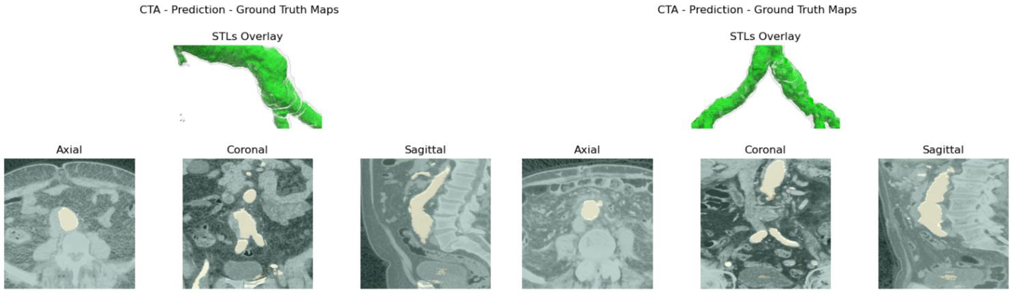
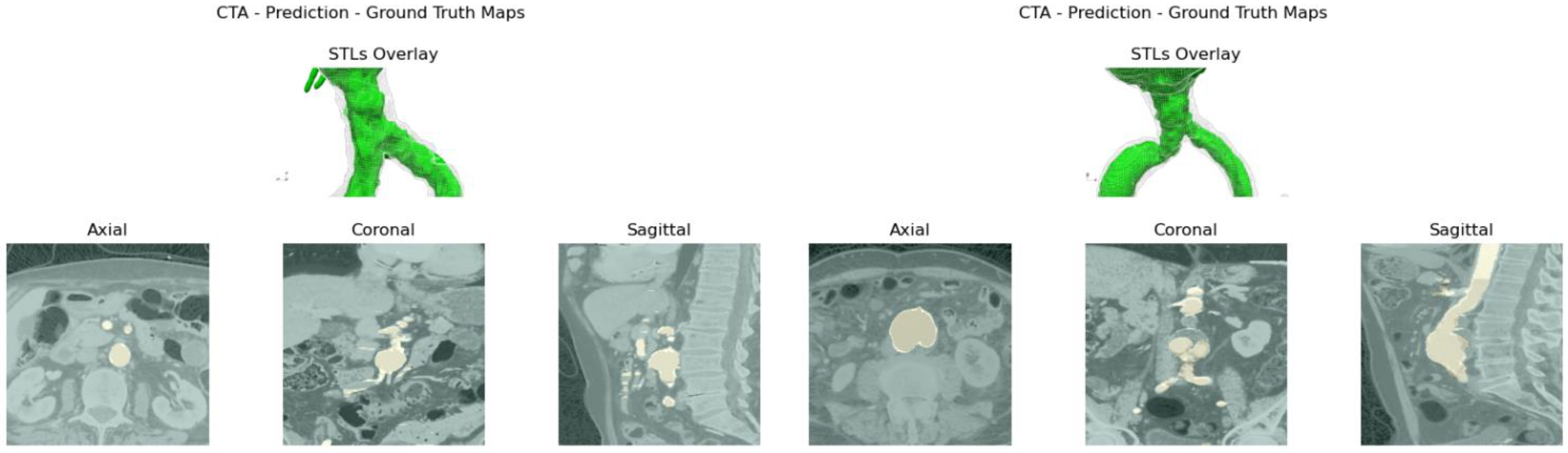
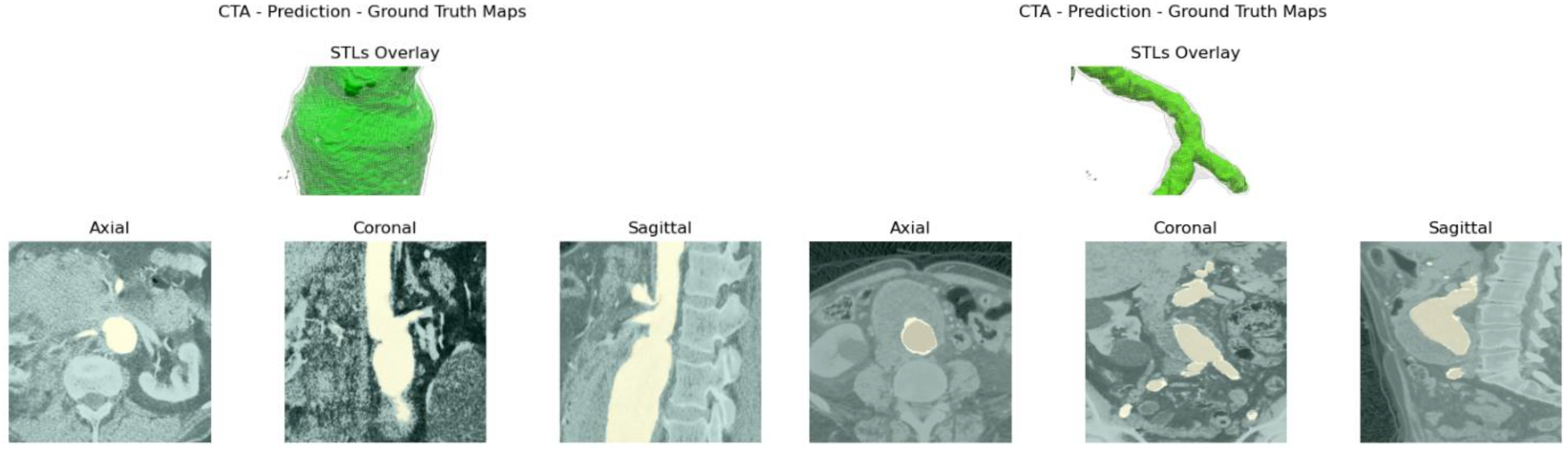
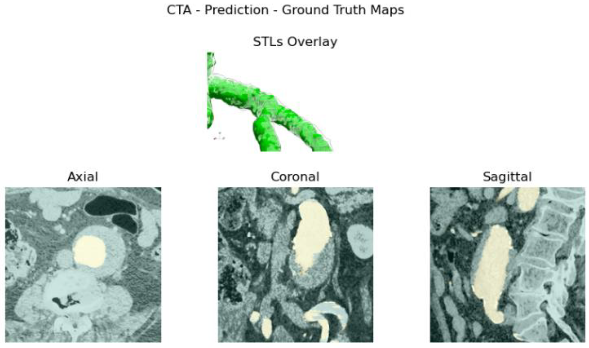
The developed test and training sets’ inclusion criteria aim to the prioritization of (i) pathologic vessels affected by abdominal aortic aneurysm, (ii) complex anatomies such as tortuous and asymmetric vessels, (iii) large abdominal aortic aneurysms with a diameter greater than 5 cm, (iv) other major aorto-iliac pathologies, and (v) data coming from different diagnostic equipment: General Electrics’ BrightSpeed, Philips’ Optima CT660, and Siemens’ Definition Edge. Patients with aortic dissection and thoracic aneurysms were not included in either of the sets. Two women and twelve men were in the test set; the mean age was 76.3 ± 5.1 . All participants included had an aneurysmatic aorta.
Each training, the evaluation and test CTA scan in the dataset were anonymized. Due to the retrospective nature of such a study and the anonymization of source data, the ethical committee did not retain necessary an ethical approval; sensible data and information were neither included nor published.
In this study, only pathologic vessels are segmented, subdividing them first into A and AC. The descriptor A indicates an aneurysmatic aorta in one or more sections/branches, e.g., iliac aneurysm, whilst AC accounts for anatomically complex pathologic vessels related to other significant complications such as stenosis, occlusion, and penetrating arteriosclerotic ulcers. To further characterize test set anatomies, two properties are set for each patients’ vessel by means of the following qualitative vessel’s properties: (i) aneurysm location and (ii) other significant pathologies. Lastly, to accurately investigate the network’s performance on feature recognition of high-interest sections, aneurysm and other pathologies’ locations are introduced as characterizing anatomical properties. In Table 1, the aforementioned classification and description of the test set’s anatomies is reported.

2.5. Surface Generation Algorithm

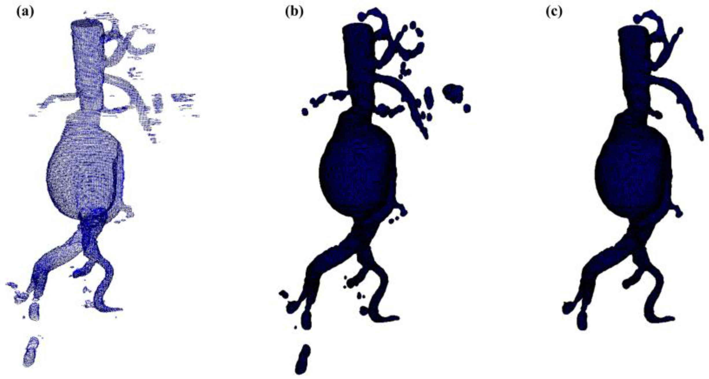
Aortic lumen 3D surface reconstruction is obtained from raw predictions using the following method: firstly, the point cloud is extracted from the predicted volume. Secondly, each axial closed contour is computed alongside its centroid. Vertex normal vectors are computed, guaranteeing correct orientation of the surface curvature, inwardly to the aortic lumen’s centerline inner point. This is mandatory to prevent holes and non-manifold, unclosed surfaces. Proceeding from bottom to top, point cloud normal are computed for each axial section of the cloud following the Python pseudo-code below:
1.
Axial single contour C i coordinates matrix [ x ¯ C i , y ¯ C i , z ¯ C i ] extraction with marching squares algorithm [19] from U-Net predictions. With x ¯ C i , y ¯ C i , z ¯ C i the column vector contains, respectively, the x, y and z coordinates of each single contour’s point. Each contour belonging to an axial section is characterized by the same z coordinate.
2.
Axial contour C i centroid extraction x j , c i = min x ¯ C i + m a x ( x ¯ C i ) 2 y j , c i = min y ¯ C i + m a x ( y ¯ C i ) 2 .
3.
Normal computation for each point of the contour C i on each section of the point cloud.
        f o r   x , y , z   i n   z i p x ¯ C i , y ¯ C i , z C i :
                              i f   z C i = = z s t a r t :
                       #Bottom patches
                        n ¯ = [ 0,0 , 1 ]
                        e l i f   z C i = = z e n d :
                       #Top patches
                        n ¯ = [ 0,0 , 1 ]
                        e l s e :
                       #Wall patches
                        n ¯ = x j , C i x C i d , y j , C i y C i d , z j , C i z C i d ,
                       with d = x j , C i x C i 2 + y j , C i y C i 2 + z j , C i z C i 2
A 3D triangulated aortic lumen surface is obtained using a screened Poisson surface reconstruction algorithm [20]. The obtained mesh is then automatically cleaned from any spurious and/or disconnected components. The algorithm is visually represented in Figure 3.

2.6. Model Evaluation

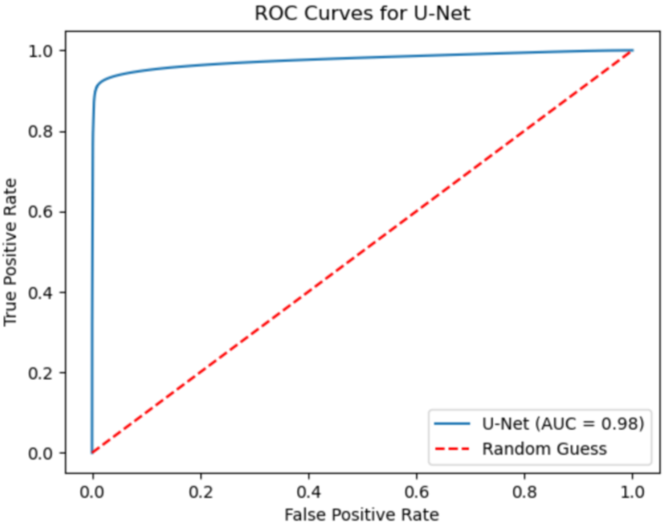
Segmentation performance is evaluated by means of IoU and F1-score metrics. Each metric is computed with its mean value and standard deviation along the total slice number. Moreover, the AOC, ROC, confusion matrix, precision and recall are also evaluated over the test set.
Robustness is assessed by perturbating the region of interest as input only. For each test CTA, the aortic lumen on nine different ROIs is predicted—one for each absolute or partial cardinal direction: C, N, S, W, E, NW, NE, SW, and SE. Each ROI volume is extracted following a fixed rule which imposes a positive or negative variation in the ROI’s origin’s coordinates. The magnitude of such a perturbation corresponds to the α = 12.5% of the ROI axial shape. To evaluate such an incremental value in pixels, one can simply perform the following: Δ = N α 100 = 32 p i x e l s , where N is the ROI’s edge dimensions in pixels. For example, the coordinates of the ROI’s center for the north (N) direction can be expressed by the following: x 0 = x 0 ,   y 0 = y 0 · ( 1 + α ) , where x 0 = 256 and y 0 = 256 are the axial section of the volume of interest’s center. It has to be underlined that the absolute origin of a single axial section is the upper left corner of the image with a positive x direction from left to right and positive y direction from top to bottom. To correctly analyze how perturbing the input ROI influences predictions’ anatomical coherence from one orientation to another proceeding slice-wise, the IoU, F1-score average and standard deviation values between predictions for the perturbed ROI along a generic direction and its relative GT are computed. The IoU and F1-score are defined as follows in Equations (1) and (2):
F 1 = 2 T P 2 T P + F P + F N
I o U = A B A B
where T P ,   F P ,   a n d   F N are, respectively, the true positives, false positives, and false negatives. A and B are, respectively, the output of the network and GT tensors. Moreover, for each patient and each ROI orientation, the global metrics’ average and standard deviation value are computed. The global average over each patient and each predicted volume obtained with ROI perturbations is also computed, following Equation (3).
m ¯ = i = 0 N p a t i e n t s j = C S E k = 0 N s l i c e s I D i m k , I D i j i = 0 N p a t i e n t s ( N o r i e n t a t i o n s · k = 0 N s l i c e s I D i m k , I D i j )
where m ¯ is the average generic metric (F1 or IoU), N p a t i e n t s is the total number of test patients, N s l i c e s I D i is the total number of slices for test patient i , m k , I D i j is the value of the generic metric at slice number k and orientation j [ N , S , W , E , N W , N E , S W , S E ] for patient i , and N o r i e n t a t i o n s = 9 is the total number of direction for the input ROI perturbations.
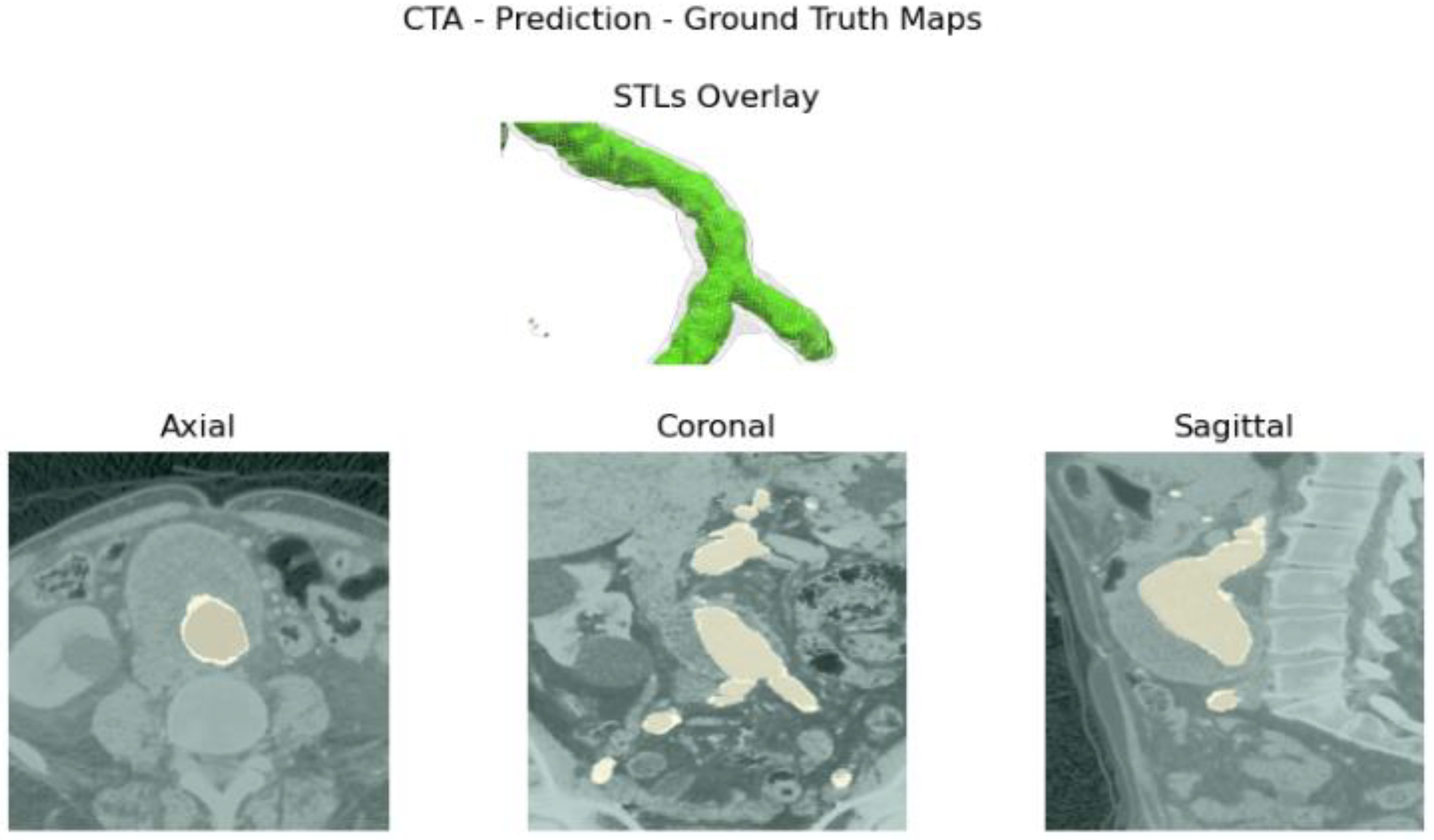
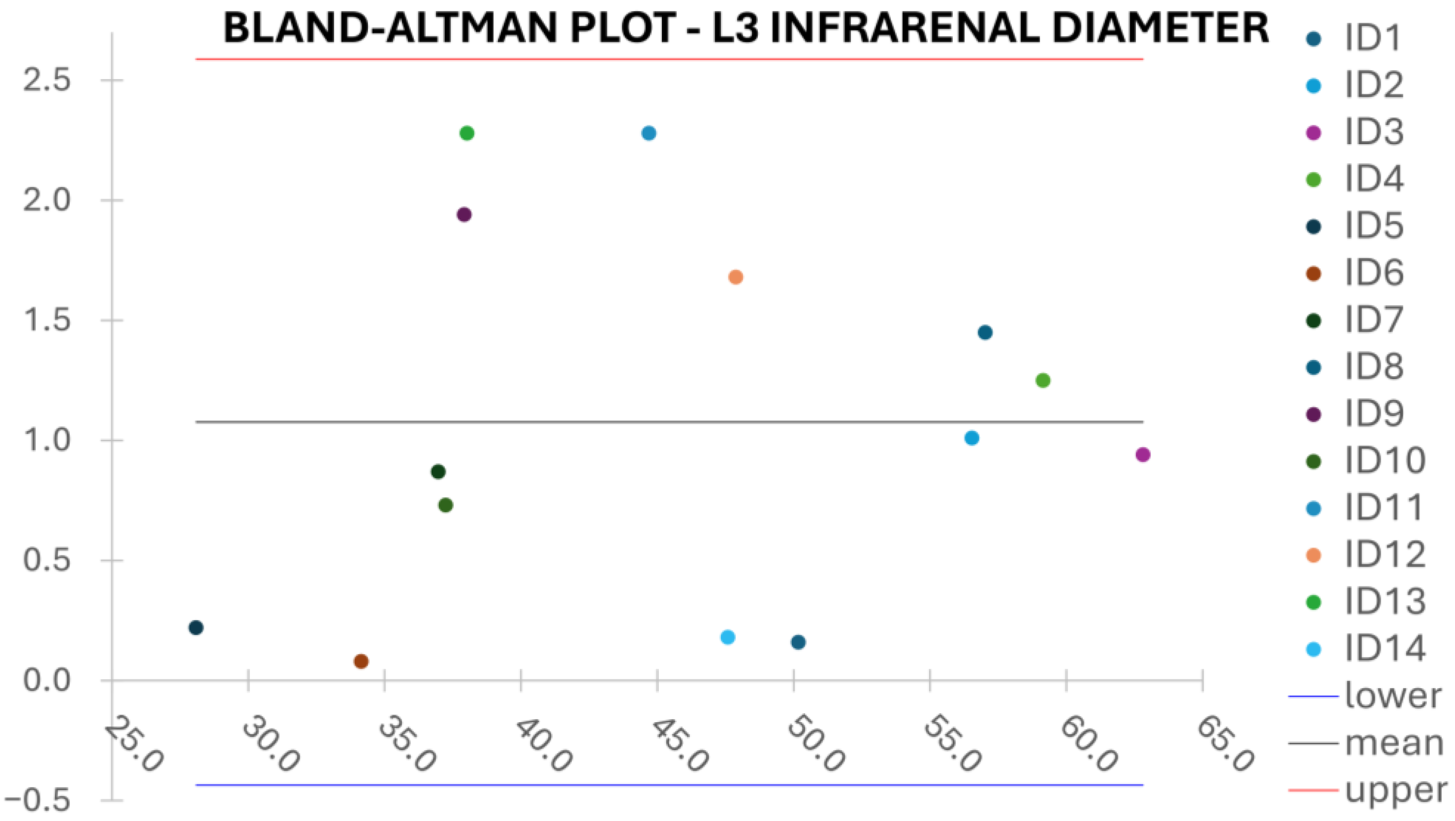
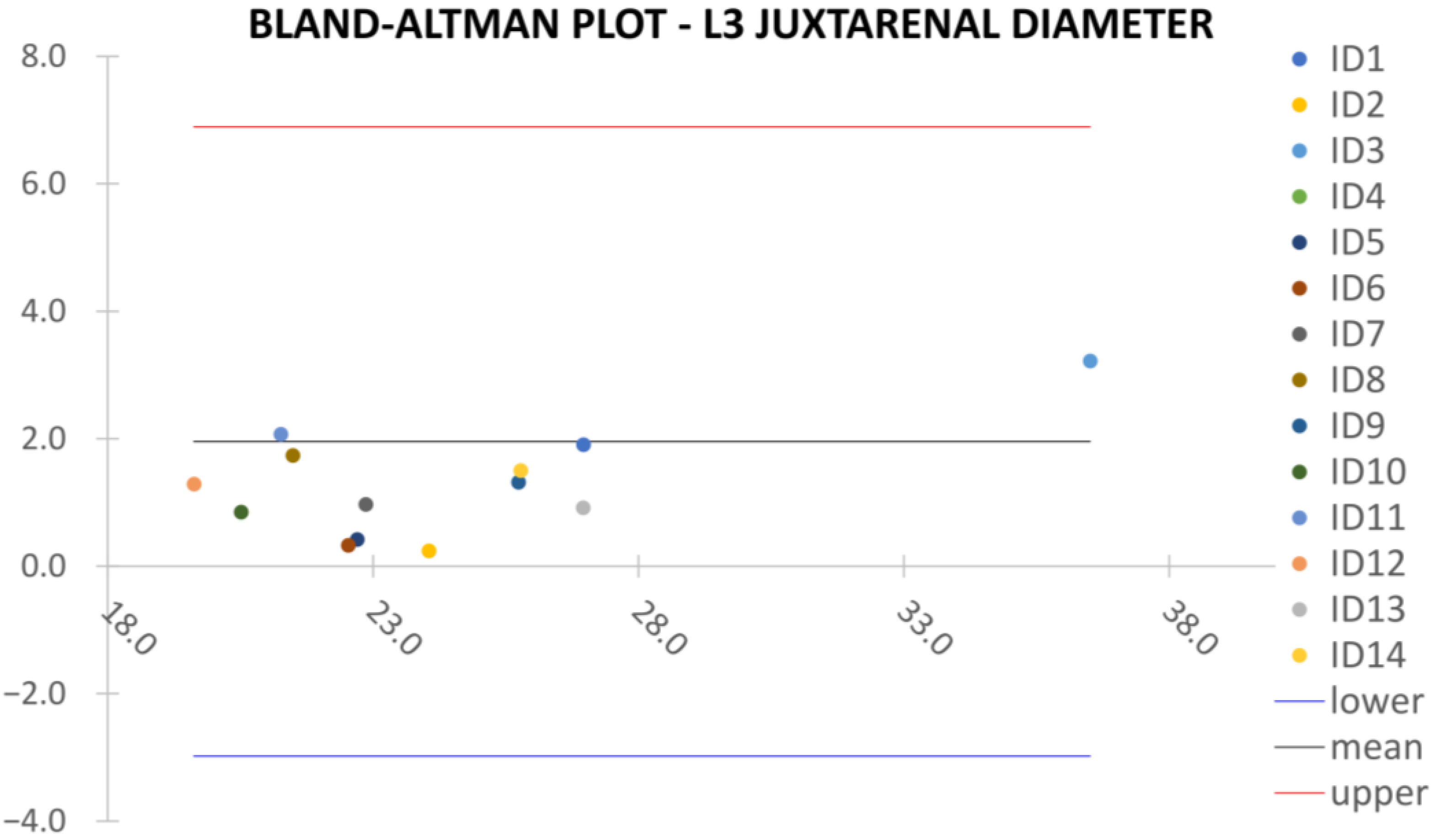
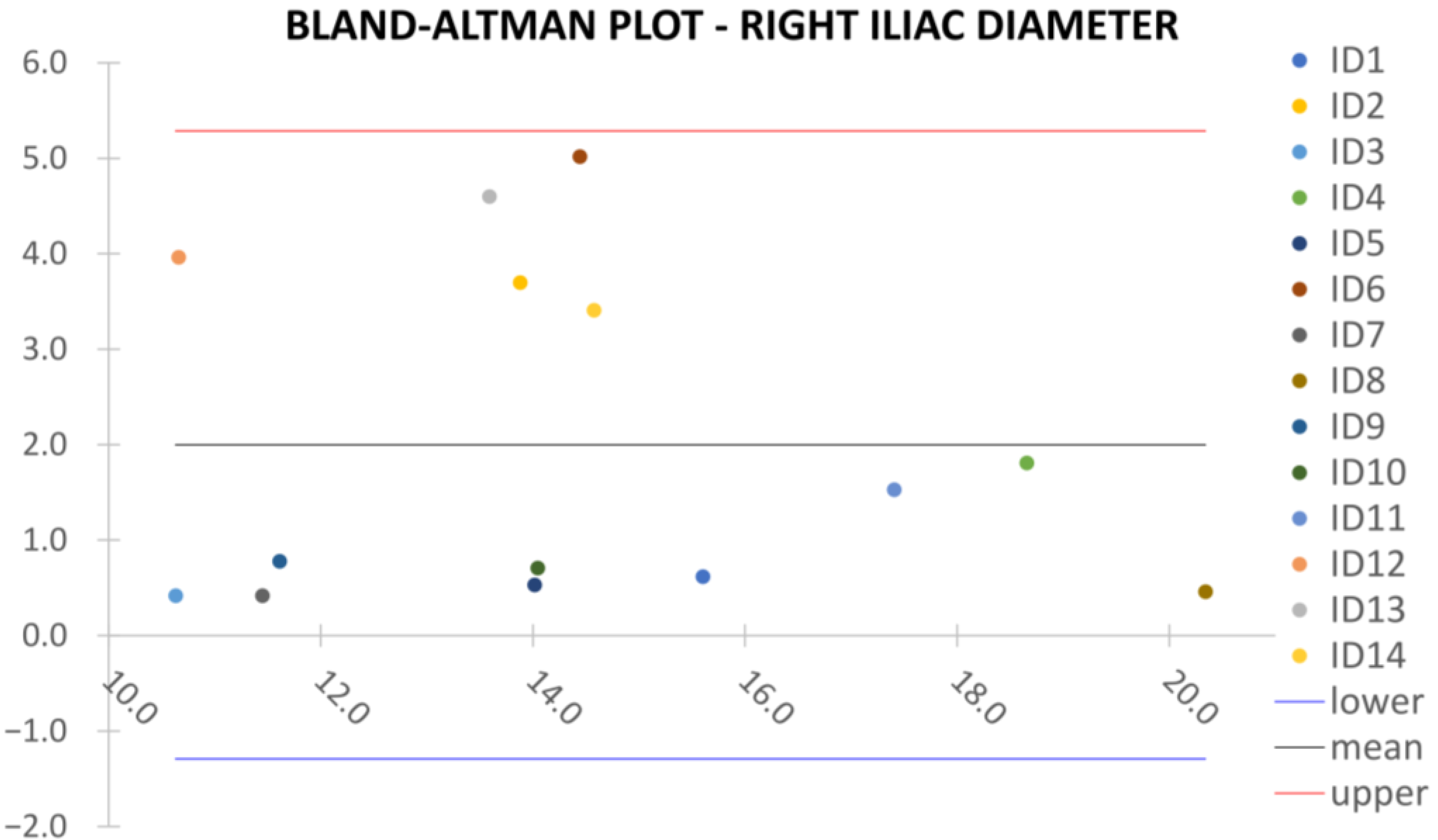
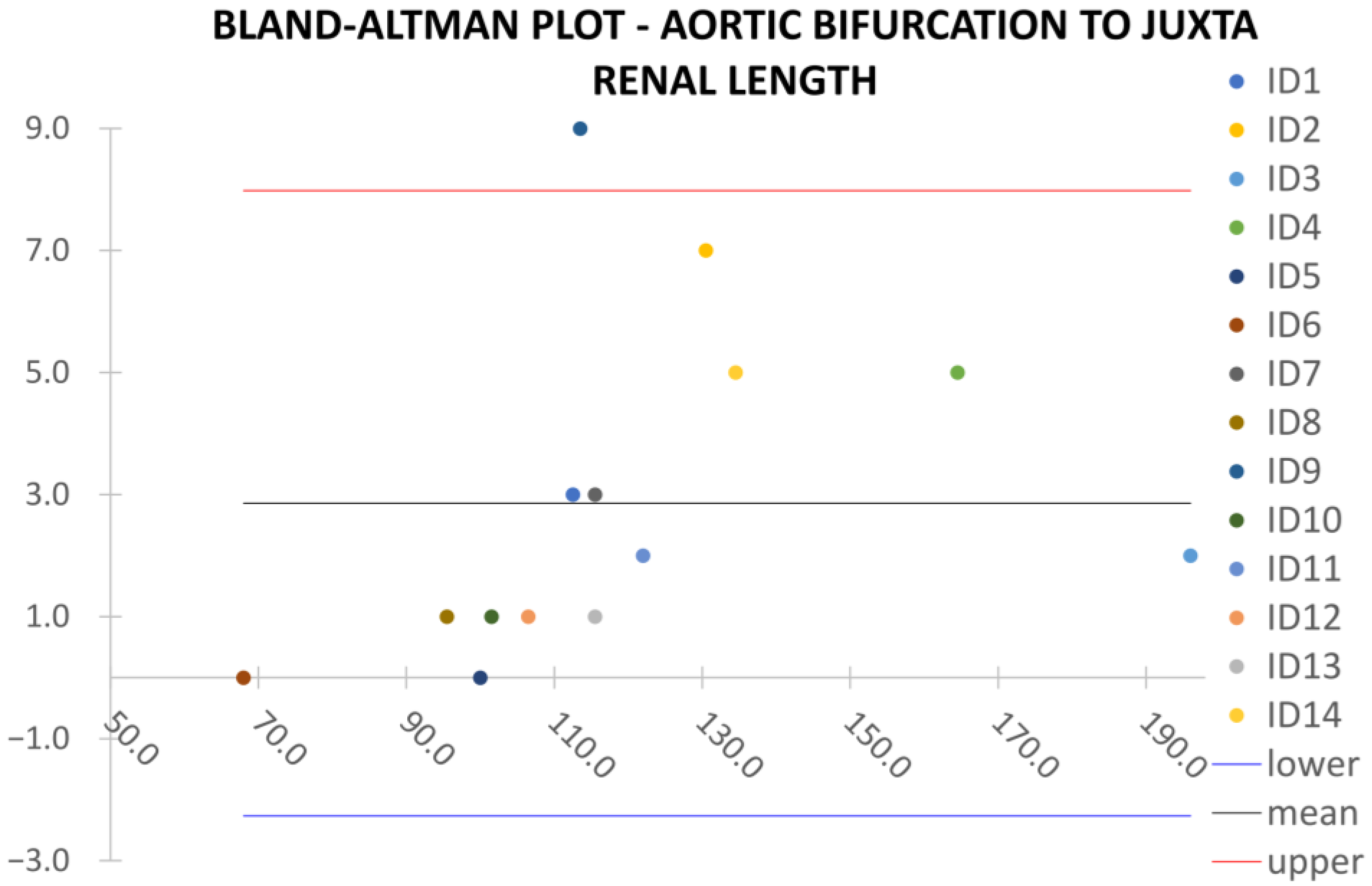
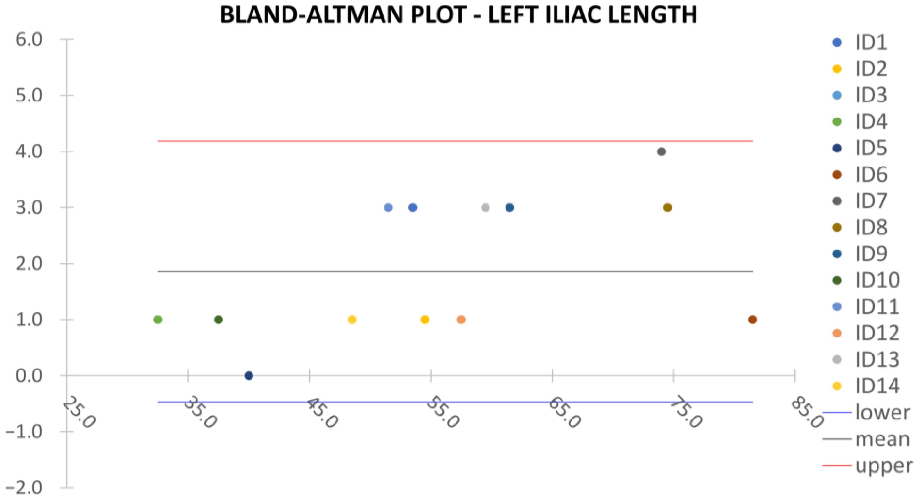
Clinical reliability is assessed by comparing centerline-based measurements performed on both the ITK-Snap and U-Net reconstructed geometries by means of absolute and relative percentage errors, as defined in Equations (4) and (5).
ϵ a = | v G T v m |
ϵ r = v G T v m v G T 100
where v G T and v m are the diameter or centerline length values, respectively, measured on ITK-Snap and U-Net 3D reconstruction geometries. Bland–Altman plots are also provided in the Appendix section from Figure A1, Figure A2, Figure A3 and Figure A4 for diameters and from Figure A5, Figure A6 and 
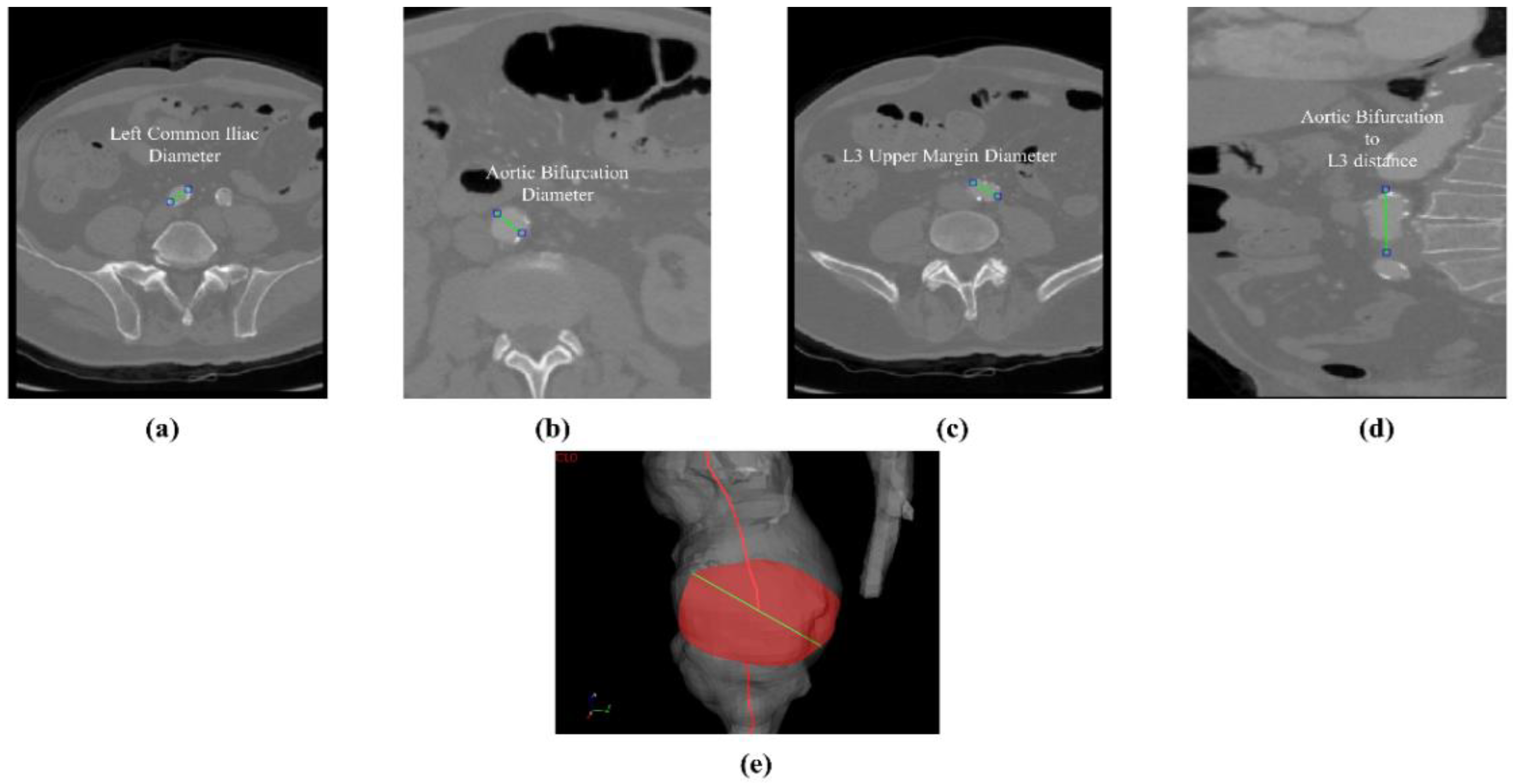
Figure A7 for the centerline’s length. Once a region of interest is reconstructed, the vessel’s centerline is computed. The user can then perform the required reference measurements, taken on a plane orthogonal to the centerline, as shown in Figure 4e. The abdominal aneurysm and iliac arteries’ lumen diameter are measured at three distinct locations:
  • Right/Left Iliac Luminal Diameter, ϕ r , i l i a c , ϕ l , i l i a c : right and left common iliac artery proximally to their bifurcation, as shown in Figure 4a.
  • L3 Infra Renal Aortic Diameter, ϕ L 3 : located on the third lumbar vertebral body’s upper margin (L3), as shown in Figure 4b, and at a distance l A B L 3 from AB, as shown in Figure 4d.
  • Juxta Renal Aortic Diameter, ϕ j u x t r : the aortic lumen immediately below the lowest renal artery, as shown in Figure 4c.
The coronal plane was used to measure the vertical distance between the aortic bifurcation and L3 body l A B L 3 , as shown in Figure 4d. The centerline-based aortic lumen’s length measure between reference sections is taken considering the following bound segments:
  • Lowest RA to Aortic Bifurcation length, L L R A B ;
  • Aortic Bifurcation to Right/Left Iliac Bifurcation, L r , A B I B , L l , A B I B .
The centerline’s length is computed as a sum of the Euclidean distances between the centerline points location as d E u = i = 1 i = N p o i n t s | r i + 1 r i | , where N p o i n t s is the total number of points of the interest centerline’s branch, and r is the position vector, which is referenced at the starting point of the centerline itself. Such a validation strategy is different from the recognized preoperative AAA measurement standards, according to the latest ESVS European Society of Vascular Surgery guidelines outlined in Wanhainen et al. [21]. To minimize measurement errors, the approach is modified and standardized by both vascular surgeon and engineers as previously described. The diameter was measured on the longest axis of the lumen from the inner-to-inner wall. Arterial thrombus and calcification were not included as the studied U-Net is of the mono-class type.
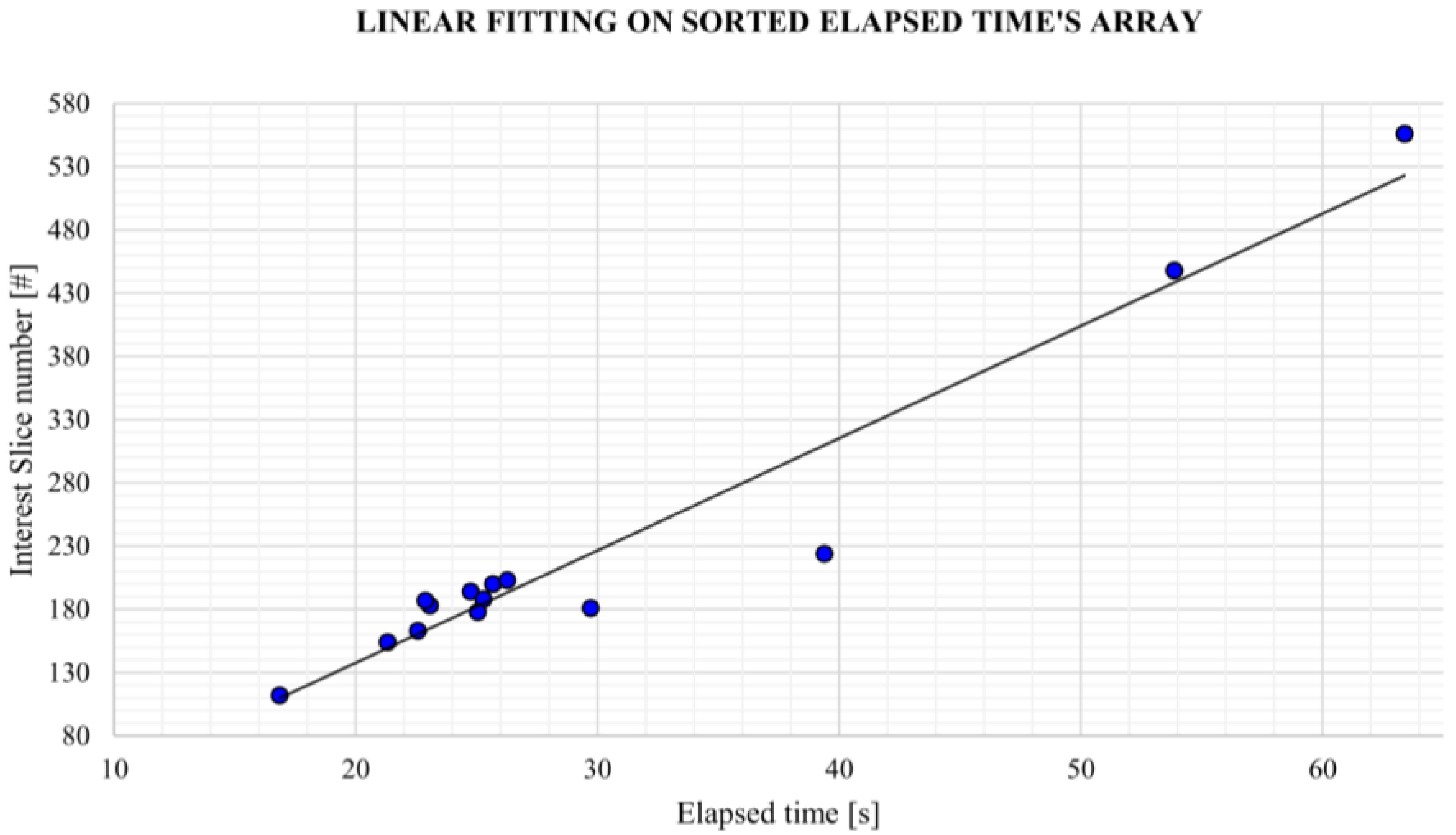
Usability and performance are also assessed by computing the average elapsed time to obtain the aortic lumen reconstruction and the average elapsed time per slice. It should be emphasized that all the reconstructions obtained by the algorithm presented in this study were retrieved from central ROI orientation predictions and CPU devices.

3. Results

3.1. Model Performance

Here, we reported three cases for performance discussion, which represent the top, average, and worst-performing cases among test sets ID_3, ID_2, and ID_12, respectively. Their performance by means of the above-mentioned metrics for each orientation are reported in Table 2, Table 3 and Table 4. Metrics for other test cases are reported in the appendix from Table A1, Table A2, Table A3, Table A4, Table A5, Table A6, Table A7, Table A8, Table A9, Table A10 and Table A11.
Case ID_3 shows the best metrics among the other patients, respectively, achieving an IoU = 0.850 ± 0.087 and an F1 = 0.916 ± 0.053 average values over each ROI perturbation. The superior mesenteric artery has been detected successfully, including the tripod. Common iliac arteries and aneurysmatic sections are also segmented correctly as well as the right common iliac PAU, as shown in Figure 5a.
Case ID_2, representing the average U-Net performance, reported an IoU = 0.810 ± 0.088 and an F1 = 0.892 ± 0.055 over each ROI’s orientation. The LIIO of such a vessel has been successfully detected. Moreover, the common iliac section and the superior mesenteric artery were also identified and reconstructed successfully, as can be seen from Figure 5b.
Case ID_12 represents the worst performance scenario, reporting an IoU = 0.752 ± 0.153 and an F1 = 0.847 ± 0.126 over each ROI’s orientation. The network provided solid and reliable results despite lower average metrics’ value and a higher standard deviation across slices. The 3D reconstruction for case ID_12 is reported in Figure 5c.
The maximum average metric’s values difference between orientations are computed for the mentioned patients, which are defined as follows:
m a v g I D _ i = m a v g , m a x I D i m a v g , m i n I D i · 100
with m a v g , m a x I D _ i and m a v g , m i n I D _ i , respectively, representing the maximum and minimum value of the average metrics among all orientations. Each of the three cases, ID_3, ID_2, and ID_12, show the small variability of the average metrics and its standard deviation across all perturbing orientations. For case ID_3, following Equation (6), Δ F 1 a v g I D _ 3 = 0.925 0.904 · 100 = 2.1 % and Δ I o U a v g I D _ 3 = 4 % (Table 2), for case ID_2 Δ F 1 a v g I D _ 2 = 2.0 % and Δ I o U a v g I D _ 2 = 3.2 % (Table 3), and for case ID_12 Δ F 1 a v g I D _ 12 = 2.5 % and Δ I o U a v g I D _ 12 = 3.5 % (Table 4). Such values indicate that the algorithm can segment the aortic lumen independently by the ROI instance, indicating coherent results with low inter-variability. To provide a better insight into the network performance on the test set, the AUC, ROC curve, and confusion matrix of the model are shown, starting with predictions and GT volumes as input data.
In Figure 6, the ROC and AUC value are plotted, showing an A U C = 0.98 . Such a value suggests excellent performance on unseen data.
In Figure 7, the confusion matrix is reported with precision p = 83.57 % and recall r = 86.75 % . For the sake of clarity, in Table 5, more detailed metrics such as the true positive, true negative, false positive, and false negative number, precision and recall are reported.

3.2. Model Reliability

A comparison between obtained measurements and those evaluated from ITK-Snap’s reference reconstructions is reported by means of absolute errors on diameters and aortic lumen’s lengths in Table 6. Single measurement’s value from reference software and U-Net surface reconstructions can be found in Table S1 Supplementary File. The worst, average and best test cases are highlighted in gray. Looking at Table 6 and the Bland–Altman plots in the Appendix, from Figure A1, Figure A2, Figure A3 and Figure A4 for diameters and to Figure A5, Figure A6 and Figure A7 for centerline length, the computed mean absolute error for reference aortic lumen diameters measurement in the juxta renal, L3 body, and left and right iliac sections is, respectively, 1.956 mm, 1.076 mm, 1.917 mm, and 1.997 mm.
The mean absolute error for the reference aortic lumen centerline’s length measurement in the aneurysm and iliac sections is, respectively, 2.857 mm, 1.857 mm, and 2.123 mm. The average absolute error obtained from the reliability assessment is, respectively, ϵ ¯ ϕ , a = 1.73   m m for diameters and ϵ ¯ l , a = 2.27   m m for the centerline’s length. In addition, from Table 7, the average relative error obtained from the reliability assessment is, respectively, ϵ ¯ ϕ , r = 10.689 % for diameters and ϵ ¯ l , r = 3.060 % for the centerline’s length.
It is clear how, for cases ID_2, ID_4, ID_6, ID_11, ID_13 and ID_14, relative errors are characterized by higher values, especially for the common iliac arteries. Considering such sections, for instance in case ID_2, the underestimation of the aortic lumen by ITK-Snap segmentation leads to higher measurement relative errors, especially for diameters, which are lower in magnitude with respect to aortic lengths. To this purpose, a detailed view of the GT and prediction masks are reported in Figure 8.
From the axial, coronal, and sagittal view, the severe underestimation cited above can be seen. For the cases reported previously, the authors present the same detailed view from Figure A8, Figure A9, Figure A10 and Figure A11, qualitatively also clarifying how U-Net segmentations are more accurate when segmenting the aortic lumen. Such a phenomenon is due to the thresholding method used in ITK-Snap to segment the aortic lumen, which in most cases underestimates the lumen area. In fact, excessively lowering the lower threshold in ITK-Snap often expands the segmentation to other undesired areas and tissues. Hence, the very first layers of the aortic lumen are eroded from the GT mask. This leads to an underestimation of the aortic lumen and consequently higher error values.

3.3. Model Usability

Elapsed time, which aims to assess usability, is computed from prediction time to the end of the 3D surface reconstruction. The average elapsed time to segment a single slice is computed through linear fitting of the elapsed time-number of slice point samples and shown in Figure 9.
The correlation between the elapsed CPU computing time and number of slices is linear with an average slope of 0.1057 s per slice. To further assess the model’s usability, the required number of inputs is accounted for as well. The user must in fact solely place the region of interest in the GUI view-box, enclosing the vessel. This peculiarity provided the model with high learnability and usability.
The correlation between the elapsed time and the number of slices showed a linear dependence: there was a minimum elapsed time of 16.86 s, average elapsed time of 27.99 s and maximum elapsed time of 63.4 s. Such information can be found in Table S2 Supplementary File. Considering the use of CPU device to obtain predictions, these processing times could be drastically reduced by adopting GPU-based computing. Although, it is better to evaluate predictions on GPUs from a time efficiency perspective, such a choice is forced by the urge to provide a general tool that is able to work under different system architectures. Elapsed time are still comparable to the ones obtained by other studies; see, e.g., Fantazzini et al. [6] and Brutti et al. [7]. Moreover, a single input ROI selection will hopefully favor learnability and widen the user spectrum.

4. Discussion

In this study, a DL-based algorithm to segment and reconstruct the abdominal aorta has been proposed. Validation has been focused on the model’s performance, robustness, reliability, and usability based on the network’s metrics and reference measurements for EVAR planning taken by a vascular surgeon. The goal was to lay the groundwork for the development of more complex enhanced diagnostic techniques and preoperative planning, which was used by medical personnel without requiring prior training. The result’s reproducibility highly reduces the risk of accidental errors, thus enhancing the overall reliability of the algorithm. Providing a complex validation pipeline for aneurysmatic aortic lumen 3D reconstruction, the proposed replicable model is considered a starting point toward an enhanced 3D aortic diagnostic framework.
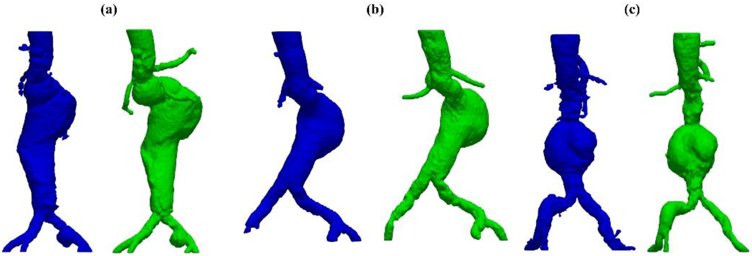
Despite some fluctuations in metrics, the network showed a good approximation of the aortic lumen, with sufficient results reproducibility and reliable 3D-based aortic measurements, even considering the uncertainty due to user input replicability. Segmentation performance analysis reports an average intersection over union and F1-score of 0.760 ± 0.150 and 0.850 ± 0.120, respectively, as well as an absolute error on aortic measurements provided and average value of ϵ a , ϕ = 1.73   m m , and ϵ a , L = 2.27   m m , respectively. Some cases are characterized by high across-slice standard deviation. However, it is crucial to bear in mind that GT extraction from CTA is performed using the ITK-Snap semi-automatic threshold segmentation mode. By proceeding this way, in certain cases, such an extraction method might exclude border pixels, which belong to the aortic lumen. This leads to an increase in false negatives, affecting the network’s performance and measurement process. The mentioned behavior can be observed in many cases: for example, cases ID_2, ID_6, ID_12, and ID_13. Moreover, a large spectrum of anatomies can determine a general decrease in test set metrics. Despite these limitations, 3D reconstructions still demonstrated good agreement with the ones obtained using the reference software.
Although this study has been conducted on a small test set, the results are overall in accordance with previous studies reporting AI-driven infra-renal abdominal aortic segmentation and automatic measurements of lumen diameter [22,23] whilst also including various anatomies and aorto-iliac pathologies. Although one may consider the average relative error high, as it exceeds the standard 5% value for the majority of cases, it has to be underlined that in the definition of relative error, the magnitude of such quantity is strongly influenced by the GT measure’s value order of magnitude. In fact, considering Equation (5), it can be seen how by keeping constant absolute errors, the value of the relative error will increase if referring to small distances, such as diameters, which lay in the 10 1 order of magnitude. Thus, to perform a fair evaluation of the dispersion between U-Net and ITK-Snap 3D measurements, this important property of the relative error’s definition must be considered, which allows the relative error uncertainty interval to be larger, as a small order of magnitude of the measure is considered. On the other hand, such behavior is negligible for the aortic section’s length, as the order of magnitude lays around 10 1 10 2 mm, as most relative errors on the aortic section’s length lay inside the 5% value.
To improve the model’s performance and reconstruction quality, the dataset’s anatomical spectrum needs to be enriched to include both wider areas and secondary vessels and particularly complex anatomies, which return unstable 3D reconstructions.
The network’s performance on secondary vessels segmentation also needs to be improved in the model’s next versions by expanding aortic lumen labeling ROI so as to include wider semantic areas. High standard deviations shown by metrics across slices can be drastically reduced by performing fine tuning on a specific subset of the training dataset which contains challenging anatomies.
The urge to obtain a model able to segment challenging data inevitably leads to taking into consideration a multi-center study. Comprising CTA scans from several institutes might boost network performance with larger and semantically richer datasets.
Future developments will involve the implementation of multi-class CNN for aortic lumen and intraluminal thrombus semantic segmentation to extend clinical usability to post-EVAR CTA scans. Intraluminal thrombus is, in fact, clinically crucial when estimating the outer maximum aortic diameter. Further steps also involve coupling a custom CFD solver to the AI model for the numerical simulation of patient-specific aortic flows which can further represent the true hemodynamic state of the diseased vessel. Quantitative hemodynamic data correlation with geometric vessel properties will enhance simulation accuracy, especially if laid on a knowledge-based semantic structure such as taxonomy or ontology, favoring digital translatability to patient-specific diagnostics addressing complex problems such as rupture risk assessment.

Supplementary Materials

The following supporting information can be downloaded at: https://www.mdpi.com/article/10.3390/biomed5020009/s1, Table S1: Aortic Measurement Results, Table S2: Elapsed Time Results.

Author Contributions

Conceptualization, E.G., E.U., G.L.C. and M.A.A.; methodology, E.G., S.S., G.L., E.U., G.L.C. and M.A.A.; software, E.U. and G.L.C.; validation, E.U., G.L.C. and M.A.A.; formal analysis, E.U. and G.L.C.; investigation, E.U., G.L.C. and M.A.A.; resources, E.G., G.R., M.G. and G.F.; data curation, E.U.; writing—original draft preparation, E.U., G.L.C. and M.A.A.; writing—review and editing, E.G., M.G., G.F. and G.R.; visualization, E.U.; supervision, E.G., S.S., G.L., M.G., G.F. and G.R.; project administration, E.G.; funding acquisition, E.G. All authors have read and agreed to the published version of the manuscript.

Funding

This research received no external funding.

Institutional Review Board Statement

Ethical review and approval were waived for this study due to the retrospective nature of the study and data full anonymization.

Informed Consent Statement

Patient consent was waived due to the data anonymization from the hospital information system.

Data Availability Statement

The data presented in this study are available on request from the corresponding author due to the current European regulations (GDPR) on privacy and data ownership (AUSL of Lecco), whose prior authorization is mandatory.

Acknowledgments

None, all authors agree with this choice.

Conflicts of Interest

The authors declare no conflicts of interest.

Abbreviations

The following abbreviations are used in this manuscript:
Aaneurysmatic
AAAabdominal aortic aneurysm
ACaneurysmatic complex
AIartificial intelligence
AUCarea under the curve
BCIbilateral common iliac
CFDcomputational fluid dynamics
CPUcentral processing unit
CTAcomputed tomography angiography
DLdeep learning
Eeast
EVARendovascular aortic repair
GPUgraphics processing unit
GTground truth
GUIgraphics user interface
IRintrarenal
JRjuxtarenal
LCIleft common iliac
LIIOleft internal iliac artery occlusion
Nnorth
NEnortheast
NWnorthwest
PAUpenetrating aortic ulcer
PRpararenal
RCIright common iliac
ROCreceiver operating characteristic
ROIregion of interest
Ssouth
SEsoutheast
SWsouthwest
Wwest

Appendix A

Appendix A.1

Figure A1. Bland–Altman plot for AL diameter using L3 vertebra height as reference plane.
Biomed 05 00009 g0a1
Figure A2. Bland–Altman plot for AL diameter using juxtarenal height as reference plane.
Biomed 05 00009 g0a2
Figure A3. Bland–Altman plot for AL diameter in left common iliac artery using aortic carrefour height as reference plane.
Biomed 05 00009 g0a3
Figure A4. Bland–Altman plot for AL diameter in right common iliac artery using aortic carrefour height as reference plane.
Biomed 05 00009 g0a4

Appendix A.2

Figure A5. Bland–Altman plot for lower renal to aortic carrefour centerline distance.
Biomed 05 00009 g0a5
Figure A6. Bland–Altman plot for aortic bifurcation to distal left iliac artery centerline distance.
Biomed 05 00009 g0a6
Figure A7. Bland–Altman plot for aortic bifurcation to distal right iliac artery centerline distance.
Biomed 05 00009 g0a7

Appendix A.3

Table A1. Mean value and standard deviation of the metrics distribution. Average performance on test set patient ID_1.
Patient ROI IoU F1
Avg STD Avg STD
ID_1 C 0.828 0.077 0.904 0.047
N 0.830 0.078 0.905 0.047
S 0.743 0.174 0.838 0.145
W 0.829 0.076 0.904 0.046
E 0.824 0.077 0.901 0.047
NW 0.830 0.078 0.905 0.047
NE 0.832 0.077 0.906 0.047
SW 0.738 0.171 0.835 0.139
SE 0.717 0.229 0.805 0.225
Table A2. Mean value and standard deviation of the metrics distribution. Average performance on test set patient ID_4.
PatientROIIoUF1
AvgSTDAvgSTD
ID_4C0.8470.0990.9130.066
N0.8440.0960.9120.062
S0.8370.1160.9060.080
W0.8550.0950.9190.062
E0.8460.1050.9130.069
NW0.8500.0920.9160.059
NE0.8430.0990.9110.064
SW0.8360.1190.9050.083
SE0.8260.1330.8980.095
Table A3. Mean value and standard deviation of the metrics distribution. Average performance on test set patient ID_5.
PatientROIIoUF1
AvgSTDAvgSTD
ID_5C0.7580.1030.8580.071
N0.7610.1010.8600.069
S0.7160.1270.8280.089
W0.7570.1080.8570.075
E0.7610.1040.8600.072
NW0.7620.1050.8610.072
NE0.7530.1110.8540.076
SW0.7070.1340.8200.096
SE0.7300.1140.8390.080
Table A4. Mean value and standard deviation of the metrics distribution. Average performance on test set patient ID_6.
PatientROIIoUF1
AvgSTDAvgSTD
ID_6C0.7480.1010.8480.072
N0.7510.1110.8500.070
S0.7260.1270.8480.090
W0.7570.1090.8670.074
E0.7610.1030.8700.071
NW0.7820.1040.8510.073
NE0.7230.1010.8440.078
SW0.7070.1240.8100.095
SE0.7100.1040.8350.075
Table A5. Mean value and standard deviation of the metrics distribution. Average performance on test set patient ID_7.
PatientROIIoUF1
AvgSTDAvgSTD
ID_7C0.7890.0920.8790.061
N0.7790.0970.8720.065
S0.7850.0940.8760.064
W0.7730.1200.8660.087
E0.7920.0910.8810.060
NW0.7510.1420.8490.104
NE0.7850.0980.8760.066
SW0.7750.1200.8670.089
SE0.7890.0940.8790.063
Table A6. Mean value and standard deviation of the metrics distribution. Average performance on test set patient ID_8.
PatientROIIoUF1
AvgSTDAvgSTD
ID_8C0.8430.0940.9110.059
N0.8410.1100.9090.080
S0.8410.1010.9100.063
W0.8290.1210.9000.094
E0.8340.1110.9040.078
NW0.8270.1320.8980.105
NE0.8280.1350.8980.103
SW0.8200.1300.8950.089
SE0.8330.1110.9040.071
Table A7. Mean value and standard deviation of the metrics distribution. Average performance on test set patient ID_9.
PatientROIIoUF1
AvgSTDAvgSTD
ID_9C0.7100.140.8210.107
N0.7110.1560.8200.119
S0.6910.1710.8030.138
W0.7020.1530.8140.116
E0.7200.1330.8300.095
NW0.7050.1580.8160.119
NE0.7180.1470.8270.109
SW0.6740.1900.7870.162
SE0.7030.1570.8150.120
Table A8. Mean value and standard deviation of the metrics distribution. Average performance on test set patient ID_10.
PatientROIIoUF1
AvgSTDAvgSTD
ID_10C0.8580.0940.9200.059
N0.8660.0770.9260.047
S0.8010.1470.8810.105
W0.8420.1430.9060.104
E0.8610.0820.9230.051
NW0.8340.1360.9020.097
NE0.8650.0770.9250.048
SW0.7810.1710.8650.124
SE0.7960.1460.8780.102
Table A9. Mean value and standard deviation of the metrics distribution. Average performance on test set patient ID_11.
PatientROIIoUF1
AvgSTDAvgSTD
ID_11C0.7710.0900.8670.063
N0.7920.0920.8810.064
S0.7760.0870.8700.060
W0.7680.0990.8650.069
E0.7790.0900.8720.063
NW0.7900.1150.8770.082
NE0.7510.1410.8490.110
SW0.7740.1090.8680.079
SE0.7800.0920.8730.063
Table A10. Mean value and standard deviation of the metrics distribution. Average performance on test set patient ID_13.
PatientROIIoUF1
AvgSTDAvgSTD
ID_13C0.7690.1300.8620.102
N0.7890.1270.8750.098
S0.7170.1500.8240.123
W0.7530.1420.8500.118
E0.7670.1330.8600.106
NW0.7790.1500.8650.126
NE0.7870.1400.8710.114
SW0.6960.1980.7990.191
SE0.7130.1640.8190.137
Table A11. Mean value and standard deviation of the metrics distribution. Average performance on test set patient ID_14.
PatientROIIoUF1
AvgSTDAvgSTD
ID_14C0.8140.1320.8910.088
N0.8170.1230.8930.080
S0.8160.1320.8920.089
W0.7810.1460.8690.102
E0.8320.1160.9030.077
NW0.7870.1350.8740.092
NE0.8330.1100.9040.072
SW0.7780.1470.8670.104
SE0.8360.1180.9050.080

Appendix A.4

Figure A8. Top: GT 3D reconstruction, in green, and U-Net 3D reconstruction wireframe (in white) overlay. Bottom: axial, coronal, and sagittal overlay of GT (in orange) and the difference between GT and U-Net predictions (in yellow) for case ID_11 (left) and case ID_13 (right).
Biomed 05 00009 g0a8
Figure A9. Top: GT 3D reconstruction, in green, and U-Net 3D reconstruction wireframe (in white) overlay. Bottom: axial, coronal, and sagittal overlay of GT (in orange) and the difference between GT and U-Net predictions (in yellow) for case ID_6 (left) and case ID_12 (right).
Biomed 05 00009 g0a9
Figure A10. Top: GT 3D reconstruction, in green, and U-Net 3D reconstruction wireframe (in white) overlay. Bottom: axial, coronal, and sagittal overlay of GT (in orange) and the difference between GT and U-Net predictions (in yellow) for case ID_4 (left) and case ID_2 (right).
Biomed 05 00009 g0a10
Figure A11. Top: GT 3D reconstruction, in green, and U-Net 3D reconstruction wireframe (in white) overlay. Bottom: axial, coronal, and sagittal overlay of GT (in orange) and the difference between GT and U-Net predictions (in yellow) for case ID_14.
Biomed 05 00009 g0a11

References

  1. Ouriel, K.; Green, R.M.; Donayre, C.; Shortell, C.K.; Elliott, J.; DeWeese, J.A. An evaluation of new methods of expressing aortic aneurysm size: Relationship to rupture. J. Vasc. Surg. 1992, 15, 12–20. [Google Scholar] [CrossRef] [PubMed]
  2. Finol, E.A.; Amon, C.H. Blood flow in abdominal aortic aneurysms: Pulsatile flow hemodynamics. J. Biomech. Eng. 2001, 123, 474–484. [Google Scholar] [CrossRef] [PubMed]
  3. Chaikof, E.L.; Brewster, D.C.; Dalman, R.L.; Makaroun, M.S.; Illig, K.A.; Sicard, G.A.; Timaran, C.H.; Upchurch, G.R.; Veith, F.J. The care of patients with an abdominal aortic aneurysm: The Society for Vascular Surgery practice guidelines. J. Vasc. Surg. 2009, 50, S2–S49. [Google Scholar] [CrossRef] [PubMed]
  4. Parkinson, F.; Ferguson, S.; Lewis, P.; Williams, I.M.; Twine, C.P. Rupture rates of untreated large abdominal aortic aneurysms in patients unfit for elective repair. J. Vasc. Surg. 2015, 61, 1606–1612. [Google Scholar] [CrossRef] [PubMed]
  5. Darling, R.C.; Messina, C.R.; Brewster, D.C.; Ottinger, L.W. Autopsy study of unoperated abdominal aortic aneurysms. The case for early resection. Circulation 1977, 56, II161–II164. [Google Scholar] [PubMed]
  6. Fantazzini, A.; Esposito, M.; Finotello, A.; Auricchio, F.; Pane, B.; Basso, C.; Spinella, G.; Conti, M. 3D Automatic Segmentation of Aortic Computed Tomography Angiography Combining Multi-View 2D Convolutional Neural Networks. Cardiovasc. Eng. Technol. 2020, 11, 576–586. [Google Scholar] [CrossRef] [PubMed]
  7. Brutti, F.; Fantazzini, A.; Finotello, A.; Müller, L.O.; Auricchio, F.; Pane, B.; Spinella, G.; Conti, M. Deep Learning to Automatically Segment and Analyze Abdominal Aortic Aneurysm from Computed Tomography Angiography. Cardiovasc. Eng. Technol. 2022, 13, 535–547. [Google Scholar] [CrossRef] [PubMed]
  8. Adam, C.; Fabre, D.; Mougin, J.; Zins, M.; Azarine, A.; Ardon, R.; d’Assignies, G.; Haulon, S. Pre-surgical and Post-surgical Aortic Aneurysm Maximum Diameter Measurement: Full Automation by Artificial Intelligence. Eur. J. Vasc. Endovasc. Surg. 2021, 62, 869–877. [Google Scholar] [CrossRef] [PubMed]
  9. Milletari, F.; Navab, N.; Ahmadi, S.A. V-Net: Fully convolutional neural networks for volumetric medical image segmentation. In Proceedings of the 2016 4th International Conference on 3D Vision, 3DV, Stanford, CA, USA, 25–28 October 2016. [Google Scholar] [CrossRef]
  10. López-Linares, K.; Aranjuelo, N.; Kabongo, L.; Maclair, G.; Lete, N.; Ceresa, M.; García-Familiar, A.; Macía, I.; Ballester, M.A.G. Fully automatic detection and segmentation of abdominal aortic thrombus in post-operative CTA images using Deep Convolutional Neural Networks. Med. Image Anal. 2018, 46, 202–214. [Google Scholar] [CrossRef]
  11. ISO/IEC 25000:2014(en); International Organization for Standardization ISO: Geneva, Switzerland, 2014. Available online: https://www.iso.org/obp/ui/#iso:std:iso-iec:25000:ed-2:v1:en (accessed on 10 February 2025).
  12. ISO/IEC 25010:2011; Software Process: Improvement and Practice 2. International Organization for Standardization ISO: Geneva, Switzerland, 2011. Available online: https://www.iso.org/standard/35733.html (accessed on 10 February 2025).
  13. Yushkevich, P.A.; Piven, J.; Hazlett, H.C.; Smith, R.G.; Ho, S.; Gee, J.C.; Gerig, G. User-guided 3D active contour segmentation of anatomical structures: Significantly improved efficiency and reliability. Neuroimage 2006, 31, 1116–1128. [Google Scholar] [CrossRef] [PubMed]
  14. van Rossum, G. Python Tutorial; Technical Report CS-R9526; Centrum Voor Wiskunde En Informatica (CWI): Amsterdam, The Netherlands, 1995. [Google Scholar]
  15. Antiga, L.; Piccinelli, M.; Botti, L.; Ene-Iordache, B.; Remuzzi, A.; Steinman, D.A. An image-based modeling framework for patient-specific computational hemodynamics. Med. Biol. Eng. Comput. 2008, 46, 1097–1112. [Google Scholar] [CrossRef] [PubMed]
  16. Moreland, K.; Ayachit, U.; Geveci, B.; Quammen, C.; Demarle, D.; Moreland, K.; Bauer, A.; Boeckel, B.; Lipsa, D.; Westphal, M.; et al. The ParaView Guide; Sandia National Laboratories: Albuquerque, NM, USA, 2016. [Google Scholar]
  17. NEMA PS3/ISO 12052; Digital Imaging and Communications in Medicine DICOM PS3.1 2016d—Introduction and Overview. National Electrical Manufacturers Association: Rosslyn, VA, USA, 2016.
  18. Ronneberger, O.; Fischer, P.; Brox, T. U-Net: Convolutional Networks for Biomedical Image Segmentation; Lecture Notes in Computer Science; Including Subseries Lecture Notes in Artificial Intelligence and Lecture Notes in Bioinformatics; Springer International Publishing: Cham, Switzerland, 2015. [Google Scholar] [CrossRef]
  19. Lorensen, W.E.; Cline, H.E. Marching Cubes: A High Resolution 3d Surface Construction Algorithm. Comput. Graph. 1987, 21, 7–12. [Google Scholar] [CrossRef]
  20. Kazhdan, M.; Hoppe, H. Screened poisson surface reconstruction. ACM Trans. Graph. 2013, 32, 1–13. [Google Scholar] [CrossRef]
  21. Wanhainen, A.; Verzini, F.; Van Herzeele, I.; Allaire, E.; Bown, M.; Cohnert, T.; Dick, F.; van Herwaarden, J.; Karkos, C.; Koelemay, M.; et al. Editor’s Choice—European Society for Vascular Surgery (ESVS) 2019 Clinical Practice Guidelines on the Management of Abdominal Aorto-iliac Artery Aneurysms. Eur. J. Vasc. Endovasc. Surg. 2019, 57, 8–93. [Google Scholar] [CrossRef] [PubMed]
  22. Caradu, C.; Pouncey, A.L.; Lakhlifi, E.; Brunet, C.; Bérard, X.; Ducasse, E. Fully automatic volume segmentation using deep learning approaches to assess aneurysmal sac evolution after infrarenal endovascular aortic repair. J. Vasc. Surg. 2022, 76, 620–630.e3. [Google Scholar] [CrossRef] [PubMed]
  23. Postiglione, T.J.; Guillo, E.; Heraud, A.; Rossillon, A.; Bartoli, M.; Herpe, G.; Adam, C.; Fabre, D.; Ardon, R.; Azarine, A.; et al. Multicentric clinical evaluation of a computed tomography-based fully automated deep neural network for aortic maximum diameter and volumetric measurements. J. Vasc. Surg. 2024, 79, 1390–1400.e8. [Google Scholar] [CrossRef] [PubMed]
Figure 1. Workflow of the proposed methodology.
Biomed 05 00009 g001
Figure 2. Schematization of the GT extraction algorithm.
Biomed 05 00009 g002
Figure 3. (a) Spurious point cloud, (b) spurious 3D aortic lumen surface, and (c) cleaned 3D aortic lumen surface.
Biomed 05 00009 g003
Figure 4. Intraluminal diameter obtained at different segments on the axial plane (cm). Left common iliac, (a) aortic bifurcation, (b) aortic diameter at the L3’s upper margin, (c) l A B L 3 distance from the upper margin of L3 body to the aortic bifurcation, (d) visual, manually measured centerline-based diameter visual sample in GUI (e).
Biomed 05 00009 g004
Figure 5. U-Net (in blue) and ITK-Snap (in green) 3D surfaces of the aortic lumen: cases ID_3 (a), ID_2 (b) and ID_12 (c).
Biomed 05 00009 g005
Figure 6. AUC value and ROC curve in test set for the U-Net.
Biomed 05 00009 g006
Figure 7. Confusion matrix of the model on test set.
Biomed 05 00009 g007
Figure 8. Top: GT 3D reconstruction (in green) and U-Net 3D reconstruction wireframe (in white) overlay. Bottom: Axial, coronal, and sagittal overlay of U-Net predictions (in yellow) and GT (in orange) for case ID_2.
Biomed 05 00009 g008
Figure 9. Linear fitting performed on sorted elapsed time array.
Biomed 05 00009 g009
Table 1. The test set anatomical and pathological classification.
Patient ID Aneurysm (Location) Pathology Class Patient
ID
Aneurysm (Location) Pathology Class
ID_1JRAAAAID_8IRAAAA
ID_2JRAAA + LIIOACID_9PRAAAA
ID_3JRAAA + RCI PAUACID_10IRAAAA
ID_4JRAAA + BCIAACID_11IRAAAA
ID_5IRAAAAID_12IRAAAA
ID_6IRAAAAID_13IRAAAA
ID_7IRAAA + LCI PAUACID_14JRAAAA
Table 2. Mean value and standard deviation of the metrics distribution. Average performance on test set patient ID_3.
PatientROIIoUF1
AvgSTDAvgSTD
ID_3C0.8570.0840.9200.051
N0.8640.0800.9250.048
S0.8410.0840.9110.051
W0.8410.0920.9110.057
E0.8620.0770.9240.046
NW0.8540.0840.9190.051
NE0.8690.0780.9280.046
SW0.8290.0920.9040.057
SE0.8330.0970.9060.061
Table 3. Mean value and standard deviation of the metrics distribution. Average performance on test set patient ID_2.
PatientROIIoUF1
AvgSTDAvgSTD
ID_2C0.8160.0840.8960.052
N0.8220.0830.9000.050
S0.7950.0870.8830.055
W0.8100.0930.8920.059
E0.8140.0890.8940.055
NW0.8250.0810.9010.050
NE0.8190.0860.8980.052
SW0.7960.0910.8830.058
SE0.7930.0940.8810.060
Table 4. Mean value and standard deviation of the metrics distribution. Average performance on test set patient ID_12.
PatientROIIoUF1
AvgSTDAvgSTD
ID_12C0.7700.1640.8590.117
N0.7780.1640.8640.117
S0.7490.1700.8440.123
W0.7710.1720.8580.125
E0.7730.1640.8610.116
NW0.7740.1740.8600.127
NE0.7780.1660.8640.119
SW0.7430.1770.8390.130
SE0.7450.1670.8420.120
Table 5. True positive, true negative, false positive and false negative number and relative percentage value.
Number (#)Percentage (%)
True Positive3,622,4731.71
True Negative207,186,59497.7
False Positive712,0050.33
False Negative553,4240.26
Total Pixel Population212,074,496100
Table 6. Absolute errors on diameters and lengths. Best performance case ID_3, average performance case ID_2, and worst performance ID_12 are highlighted in gray.
DIAMETERS   ϕ   AND   CENTERLINE   LENGTHS   L i —ABSOLUTE ERRORS [mm]
Patient ϕ j u x t r ϕ L 3 ϕ l , i l i a c ϕ r , i l i a c L L R A B L l , A B I B L r , A B I B
ID_11.9100.1603.0001.0000.6201.2603.000
ID_20.2401.0101.0001.0003.7002.4207.000
ID_33.2200.9401.0001.0000.4200.5802.000
ID_410.6101.2501.0001.0001.8107.1105.000
ID_50.4200.2200.0002.0000.5300.4300.000
ID_60.3300.0801.0008.0005.0205.2200.000
ID_70.9700.8704.0000.0000.4201.0003.000
ID_81.7401.4503.0000.0000.4600.6701.000
ID_91.3201.9403.0004.0000.7800.6709.000
ID_100.8500.7301.0003.0000.7100.1201.000
ID_112.0702.2803.0001.0001.5300.7202.000
ID_121.2901.6801.0002.0003.9603.1601.000
ID_130.9202.2803.0003.7284.6002.4001.000
ID_141.5000.1801.0002.0003.4101.0905.000
Table 7. Relative errors on diameters and lengths. Best performance case ID_3, average performance case ID_2, worst performance ID_12 are highlighted in gray.
DIAMETERS   ϕ   AND   CENTERLINE   LENGTHS   L i —RELATIVE ERRORS [mm]
Patient ϕ j u x t r ϕ L 3 ϕ l , i l i a c ϕ r , i l i a c L L R A B L l , A B I B L r , A B I B
ID_17.3430.3183.8968.8852.6315.4541.960
ID_21.0021.80230.75620.1335.2231.8181.408
ID_39.2261.4854.0305.1641.0152.7021.785
ID_440.5112.13610.19752.9012.9943.1252.325
ID_51.8670.7863.8542.2300.0000.0003.508
ID_61.4750.23442.07854.2620.0001.2199.756
ID_74.3342.3813.7365.8482.6315.2630.000
ID_88.4382.5752.2873.0301.0413.9470.000
ID_95.2635.2506.9516.6607.6274.7617.415
ID_104.2311.9795.1860.8270.9902.6315.368
ID_1110.2325.2348.4204.0721.6526.0002.439
ID_126.7963.57145.62228.4680.9341.7244.166
ID_133.3556.18240.74420.7970.8624.9187.652
ID_145.6540.37726.4957.0453.6492.0833.846
Disclaimer/Publisher’s Note: The statements, opinions and data contained in all publications are solely those of the individual author(s) and contributor(s) and not of MDPI and/or the editor(s). MDPI and/or the editor(s) disclaim responsibility for any injury to people or property resulting from any ideas, methods, instructions or products referred to in the content.

