Article

Simplified Cost Functions Meet Advanced Muscle Models to Streamline Muscle Force Estimation

by
Muhammad Hassaan Ahmed
1,2,
Jacques-Ezechiel N’Guessan
1,2,
Ranjan Das
1,
Matthew Leineweber
3,* and
Sachin Goyal
1,2,*
1
Department of Mechanical Engineering, University of California, 5200 Lake Road, Merced, CA 95343, USA
2
Health Science Research Institute, University of California, 5200 Lake Road, Merced, CA 95343, USA
3
Biomotum, 3025 SW 1st Avenue, Portland, OR 97201, USA
*
Authors to whom correspondence should be addressed.
BioMed 2024, 4(3), 350-365; https://doi.org/10.3390/biomed4030028
Submission received: 4 July 2024 / Revised: 13 September 2024 / Accepted: 14 September 2024 / Published: 19 September 2024

Abstract

:
Background/Objectives: This study explores an optimization-based strategy for muscle force estimation by employing simplified cost functions integrated with physiologically relevant muscle models. Methods: Considering elbow flexion as a case study, we employ an inverse-dynamics approach to estimate muscle forces for the biceps brachii, brachialis, and brachioradialis, utilizing different combinations of cost functions and muscle constitutive models. Muscle force generation is modeled by accounting for active and passive contractile behavior to varying degrees using Hill-type models. In total, three separate cost functions (minimization of total muscle force, mechanical work, and muscle stress) are evaluated with each muscle force model to represent potential neuromuscular control strategies without relying on electromyography (EMG) data, thereby characterizing the interplay between muscle models and cost functions. Results: Among the evaluated models, the Hill-type muscle model that incorporates both active and passive properties, combined with the stress minimization cost function, provided the most accurate predictions of muscle activation and force production for all three arm flexor muscles. Our results, validated against existing biomechanical data, demonstrate that even simplified cost functions, when paired with detailed muscle models, can achieve high accuracy in predicting muscle forces. Conclusions: This approach offers a versatile, EMG-free alternative for estimating muscle recruitment and force production, providing a more accessible and adaptable tool for muscle force analysis. It has profound implications for enhancing rehabilitation protocols and athletic training, not only broadening the applicability of muscle force estimation in clinical and sports settings but also paving the way for future innovations in biomechanical research.

1. Introduction

Human motion is powered by the activation of the skeletal muscles, which respond to electrochemical signals from the nervous system. The adult human musculoskeletal system, consisting of approximately 350 joints and more than 650 named muscles, presents a complex system for sharing muscle forces [1,2]. In particular, many muscle groups control the same degree of freedom (DoF) across multiple joints, leading to an over-actuated system, where an infinite number of possible muscle force distributions can generate the same net torque forces at the joints. Therefore, estimating muscle forces solely based on torque data at the joints poses a conceptual modeling challenge [3,4].
The brain plays a pivotal role in the activation of muscles, ensuring that they work harmoniously to produce the desired movement. A fundamental question in musculoskeletal modeling is how the brain activates these muscles to manage such an over-actuated system. Typically, researchers mimic this process through optimization strategies that involve designing cost functions. The purpose of these cost functions is to reflect the role of the central nervous system in governing muscle recruitment, either by directly representing physiological processes or using abstract mathematical formulas that are not directly related to physiological functions to minimize or maximize some criterion [5]. These optimization strategies help address redundancy in muscle activation, approximating a strategy to distribute the torque contributions of each muscle based on predefined assumptions [6,7]. Computational techniques such as static optimization [8] and muscle synergy concepts [9,10] are employed to improve model accuracy.
The actual mechanisms by which the central nervous system controls muscle activation are still largely unknown. Consequently, various theoretical cost functions have been proposed to approximate these neuromuscular control strategies [11,12,13,14]. Some of these functions aim to simulate the complex biochemical pathways influencing muscle contractions [15], while others focus on minimizing mechanical energy across movements [16]. Although trends have evolved towards developing sophisticated cost functions, the relationship between the complexity of the cost functions and the accuracy of the results is not definitive. In fact, simpler mechanics-based cost functions such as Sum of Muscle Forces, Sum of Stresses and Sum of Work have also produced results that align closely with the experimental data [17]. Furthermore, in contexts where speed, ease of implementation, and clarity are crucial, such as educational uses, performance evaluations, or preliminary analyses, simpler, more intuitive cost functions may become necessary or at least be more advantageous.
Recent work has proposed cost functions that leverage both kinematic and electromyography (EMG) data to calculate the force distribution across muscle movements [18]. This approach effectively minimizes mechanical stress and accounts for muscle co-contractions by aligning model predictions closely with empirical EMG results. Although this methodology has advanced our understanding of muscle dynamics, it does not consider alternative cost function strategies that focus on minimizing individual muscle forces, muscle force per physiological cross-sectional area (PCSA), or mechanical work produced by each muscle [19,20,21,22]. Furthermore, EMG measurements face challenges due to the inaccessibility of deep muscles and the presence of signal noise, even for superficial muscles [23,24]. These limitations hinder the practicality of EMG-based methods in many applications. Our study builds on the foundational work on mechanics-based cost functions by examining simpler EMG-free alternatives in conjunction with detailed muscle models, with the aim of enhancing both the accessibility and applicability of muscle force estimation across various domains.
In this study, we use a simple one DoF bicep curl model to explore how different muscle models and cost functions influence the distribution of muscle force. Our goal is to demonstrate that even less complex cost functions can yield highly accurate muscle force estimates when combined with detailed muscle models. We evaluated three muscle models of increasing complexity: (a) a Simple force model with two contact points [6,17], (b) a Hill-type muscle model incorporating active force–length and force–velocity relationships [25], and (c) a Hill-type model that also includes passive force–length relationships [16]. We pair these models with the minimization of three different cost functions that do not require EMG data: (a) total muscle force [17,19,22], (b) total work performed by the muscles [20], and (c) total stress developed in the muscles, where stress is the force per physiological cross-sectional area (PCSA) of the muscle [12,17,21,22]. The choice of cost function is based on its suitability for the specific muscles and tasks involved, as noted in the literature [6]. For example, minimizing total muscle force is appropriate for tasks aimed at reducing fatigue, such as rehabilitation exercises, where preventing overuse of specific muscles is crucial and stress minimization is often used in arm muscle modeling [6,18,26], whereas energy expenditure minimization is preferred in leg muscles for gait analysis [6,15,27]. We evaluate the efficacy of each model and the cost function combination by comparing the computed muscle and arm moments with the established elbow flexion data. This comparison assesses the accuracy of our models and helps identify the most effective strategies to simulate realistic muscle actions.

2. Methodology

To explain our methodology, we begin by describing the biomechanical model for the bicep curl motion with one degree of freedom (DoF) (see Section 2.1), which we use to investigate the impact of different combinations of muscle activation models and optimization strategies on muscle force estimation. Next, in Section 2.2, we detail the process for calculating the forces and torque required at the elbow joint for the curling motion. We then examine various muscle models (detailed in Section 2.3) and cost functions (outlined in Section 2.4), which we employ to estimate the forces generated by the elbow flexors, taking into account an applied load and the prescribed angular velocity of the curl. Finally, Section 2.5 describes how we validated our model results.

2.1. Biomechanical Model

The biomechanical model of the arm was developed using MATLAB Simscape Multibody (version 4.16, The Mathworks, Natick, MA, USA), as a multibody system with two linked segments representing the upper arm (humerus) and the forearm. The elbow joint, comprising the radiohumeral, ulnohumeral, and proximal radioulnar joints, primarily allows two degrees of freedom (DoF): flexion/extension (bending and unbending of the elbow) and pronation/supination (twisting the forearm about its longitudinal axis) [28]. However, the bicep curl is dominated by flexion/extension and therefore in this study the joint was approximated to have a single DoF, similar to a single-axis hinge.
The geometric and inertial parameters of the forearm were obtained from existing literature [15,17] and are summarized in Table 1. The model includes the three primary flexor muscles of the elbow: the biceps brachii (bic), brachialis (bra) and brachioradialis (brd). The origins, insertions, and orientations of the muscles relative to the linked segments are shown in Figure 1 and detailed in Table 1 [29,30,31]. The orientation of each muscle is characterized by the parameter α i , where i refers to the muscles: bic, bra, or brd. This parameter α i represents the acute angle between the line of action of the muscle force and the longitudinal axis of the forearm. Angle α i determines the moment arm for each muscle, influencing the calculation and behavior of the muscle forces during motion.
In our simulation case study, we consider a range of forearm rotations, in which the angle θ varies from 15° to 120° (see Figure 1). The forearm is considered to rotate at a constant angular velocity ω while carrying a mass W = 30 N . The endpoints of each muscle remain fixed, while their lengths and orientations change dynamically. Forces and moments at the elbow joint were calculated using a dynamic multibody system formulation, in which the upper arm (humerus) remains stationary in a vertical configuration and only the forearm moves.

2.2. Calculation of Forces and Torque at the Elbow Joint

We perform an inverse dynamic analysis [32] to compute the unique joint forces and moments at the elbow for the desired curl, which will then be used to estimate the muscle force distribution. Although the joint moment has contributions solely from the muscles, the joint forces include contributions both from the muscles and from interactions between the bones.
The Newton–Euler equations governing the motion of the multi-body system are generally encapsulated by
M q ¨ = G ( q , q ˙ ) ,
where, in our case,
[ M ] = m 0 0 0 m 0 0 0 μ
is the inertia matrix (m is the mass of the forearm and μ is the moment of inertia specified in Table 1), and
{ q } = x y θ
is the vector of generalized coordinates. Here x and y are the coordinates of the center of mass (CM) of the forearm and θ is the angle that the body-fixed vector a ^ 1 makes with the global vector e ^ 1 as shown in Figure 1. Quantities q ˙ and q ¨ are the generalized velocities and accelerations, respectively, and G ( q , q ˙ ) represents the generalized forces that make up the equivalent force system at the center of mass, of the constraint (joint) forces and moment that we intend to compute, as well as the applied loads. In our case,
{ G } = 0 m g W W ( L L c g ) sin θ   +   λ 1 λ 2 T λ 1 L c g cos θ λ 2 L c g sin θ ,
where the first part captures the contribution of the applied loads (the load W carried by the arm and the weight m g of the forearm itself) and in the second part, the Lagrange multipliers λ 1 and λ 2 are the forces at the elbow joint and T is the joint torque that we intend to compute. Here L is the length of the forearm and L c g is the distance of CM from the elbow specified in Table 1. The elbow, considered a revolute joint, imposes a set of constraints that are appended by a driving constraint of constant angular velocity ω = θ ˙ of the forearm. These constraints are described by the following set of expressions that are all set to zero.
{ Φ } = x L c g cos θ y + L c g sin θ θ ω t θ ° ,
where, θ ° is the starting elbow angle, which is π 12 and t is the time. Setting each of the expressions of { Φ } to zero, the generalized coordinates q that describe the arm configuration are solved at each time instant. Then, the generalized velocities q ˙ and generalized accelerations q ¨ are solved at each time instant using
q ˙ = Φ q 1 Φ t
and
q ¨ = Φ q 1 γ ,
where
γ = ( Φ q q ) q q ˙ + 2 Φ q t q ˙ + Φ t t ,
Φ q = J a c o b i a n Φ , q is the constraint Jacobian and likewise Φ t = J a c o b i a n Φ , t , Φ q t = J a c o b i a n Φ q , t , and so on depending on the subscripts in the notation.
The time series of q, q ˙ and q ¨ solved using the above-mentioned steps are then substituted in Equation (1) to get time series of the joint forces λ 1 and λ 2 and the torque T. To estimate the muscle forces that contribute to these joint forces and moment, the muscle model needs to be considered, which are presented in the next section.

2.3. Muscle-Force Models

In this study, we evaluated the performance of three skeletal muscle force generation models, listed below in order of increasing complexity and physiological accuracy:
1.
Simple Force Model [33]:
This model considers muscle force as a vector directed from its insertion to its origin, without considering the effects of the skeletal muscle’s force–length relationship or the speed of muscle contraction. Since this model does not attempt to address the physiological properties of skeletal muscle, it serves as a control from which the effects of more complex models can be evaluated.
2.
Hill-Type Active Model [25]:
Hill-type models have been widely used as a foundational representation of skeletal muscle mechanics, incorporating the effects of muscle fiber length and contraction speed to estimate maximum force generation [25]. The muscle force equation is:
F m ( t ) = F m a x i s o · a m ( t ) · f a ( l m ) · f v ( l v ) ,
where F m a x i s o represents maximum isometric force, a m ( t ) is muscle activation, f a ( l m ) captures the active force–length relationship and f v ( l v ) captures the force–velocity relationship.
3.
Hill-Type Active and Passive [34]:
This comprehensive model builds on the Hill-Type Active model to represent both active and passive muscle contraction behaviors [34]. The muscle force is given by:
F m ( t ) = F m a x i s o · [ a m ( t ) · f a ( l m ) · f v ( l v ) + f p ( l m ) ] .
Here, the additional term f p ( l m ) represents the passive force–length property, adding another layer of complexity by considering the intrinsic force–length properties of muscle fibers.
The active and passive force–length properties are expressed in [25,35] as
f a ( l m ) = e c l m l o p t , m l o p t , m w 3
and
f p ( l m ) = e 10 l m l o p t , m 15
respectively, where l m is the muscle fiber length, l o p t , m is the optimum muscle fiber length to produce maximum force, w determines the width and is set as 0.4 and c is a coefficient set as ln ( 0.05 ) .
The force–velocity property for muscle shortening is given as [35]:
f v ( l v ) = 12 l o p t , m l m ˙ 12 l o p t , m + K l m ˙ , l m ˙ < 0
where l ˙ m is the muscle lengthening velocity and K is the curvature constant and is set to 5. Both Active only and Active & Passive Hill-Type muscle models rely on the force–length relationships of both muscle fibers as well as tendons. These relationships are challenging to model due to their nonlinear nature and dynamic changes during contraction. Accurately determining muscle fiber length at each time step is particularly challenging, as the total muscle length includes both muscle fibers and tendons, which change non-linearly. To address these issues, our approach uses known optimal muscle lengths and angle α i as starting points to model muscle and tendon behavior.
Additionally, simplifications and assumptions regarding elasticity and stiffness are applied to represent muscle and tendon behaviors. These modifications simplify the model while retaining essential characteristics of the muscle-tendon system, thus allowing for the development of models that can reasonably estimate muscle forces and their interactions within the system, despite the complexities of nonlinear force–length relationships and variable lengths during contraction. The following adaptations are often made to address specific modeling challenges.
Constant tendon length—In this approximation, muscle lengths exceed realistic bounds, and force–length properties are inaccurately represented at the beginning and end of the motion.
Linear muscle contraction—In this adaptation, the muscle length is assumed to change at a constant rate. As a result, however, the force–velocity value is constant and is not correctly represented.
Linear tendon length change—In this adaptation, while the rate of tendon length change remains constant, muscle length changes non-linearly, providing more realistic force–length and force–velocity values.
Exponential tendon length change—In this one, the rate of change of tendon length varies exponentially, offering the most accurate representation of the muscle model.
A comparative analysis between the Linear and Exponential Tendon Length approximations reveals that the force–length and force–velocity values closely match the actual data observed during the bicep curl motion from 15° to 120° [36]. Consequently, we chose the Linear Tendon Length approximation for our simulation case study. This choice simplifies the modeling process while still producing results that closely align with the observed force–length and force–velocity characteristics during the curling motion, and thus effectively balances accuracy with computational efficiency, making it suitable for our intended purpose.

2.4. Muscle-Force Constraints and Cost Functions

The single DoF of elbow flexion represented by angle θ is controlled by three muscles (bic, bra, brd) which independently exert forces to produce torque around the elbow joint. This setup allows infinite combinations of muscle force distributions to achieve the same movement. This over-actuation presents a challenge in uniquely identifying the muscle forces that must undergo some constrained optimization. Although the net joint torque T required to perform the motion can be uniquely derived from the way θ evolves using the inverse dynamic approach, identifying the specific contributions to the torque of the forces exerted by each muscle group on the forearm ( F b i c , F b r a , F b r d ) is challenging due to the lack of sufficient equations. These forces are related to the torque T as follows:
r b i c × F b i c + r b r a × F b r a + r b r d × F b r d = T e ^ 3 ,
where each term is a cross-product of position vector r i of i-th muscle’s insertion point on the forearm relative to the elbow joint with the corresponding muscle force. To solve the inverse problem of finding muscle forces from the above equation, optimization approaches and constraints that appropriately narrow down the range of possible force combinations are needed.
One constraint applied in this study involves the maximum isometric force that each muscle can produce, which sets upper limits for muscle forces. This constraint is expressed through the inequality:
0   | F i |   F m a x , i ; i [ b i c , b r a , b r d ] ,
where F m a x , i represents the maximum force that the i-th muscle can exert. The values for the maximum isometric forces for the bic, bra, and brd muscles were taken from existing literature [34]. Depending on the muscle model used, additional constraints on muscle force combinations vary: (a) for the Simple Force Model, no further constraints are applied; (b) for the Active Hill-Type Model, muscle forces are constrained by active force–length and force–velocity relationships, as specified in Equations (11) and (12); (c) for the Active and Passive Hill-Type Model, the constraints include active force–length, passive force–length, and force–velocity properties, detailed in Equations (11)–(13).
These constraints restrict the range of possible solutions, and so a cost function must be applied to find a unique solution. This study evaluates the three different cost functions listed in Table 2: J 1 , which captures the total muscle force exerted [17,19,22], J 2 , which defines the total work done by the muscles [20], and J 3 , which is the total stress developed in the muscles, the stress being the force per physiological cross-sectional area (PCSA) of each muscle [12,17,21,22]. The values for P C S A m , i were obtained from references [37,38], ensuring that the calculations are based on established biomechanical data. Cost function J 1 is minimized via linear least-squares approach using MATLAB command lsqlin [39], while J 2 and J 3 are minimized as constrained nonlinear multivariable functions using MATLAB command fmincon [40].

2.5. Model Validation

For this study, we conducted validation by comparing the calculated moment arms and muscle moments for each muscle with data from previously published studies. In particular, the comparison utilized moment arm data from a diverse subject pool (both male and female) captured during elbow flexion movements, starting from 25° and extending to 110° as documented in reference [41]. Additionally, muscle moment data spanning an extended range of elbow flexion from 0° to 120° were used for further validation [42]. Our model specifically simulates elbow flexion from 15° to 120°, making it compatible with the ranges used in these studies for a comprehensive comparative analysis. The angular velocity of the elbow joint within our model simulation was held constant at ω = 1.5 rad / s , which is slow enough to reduce dynamic effects and expect the results to be in the ballpark with the benchmarks cited above.
To get an effective dimensionless comparisons between the results, the moment arm and muscle moments were normalized.

3. Results

This section details the results of our simulations, analyzing the generated joint torques and muscle forces during elbow flexion. We begin by exploring the torque dynamics required to rotate the elbow from 15° to 120° in Section 3.1, highlighting changes throughout the motion. Subsequently, in Section 3.2 we evaluate muscle forces under three modeling scenarios: the Simple Force Model, which serves as a baseline; the Hill-Type Active Model, which incorporates active force–length relationships for a more realistic muscle behavior; and the Hill-Type Active and Passive Model, which further integrates passive force properties to enhance model accuracy. In Section 3.3, we validate our model by comparing our predictions with published data, focusing on muscle moments and their moment arm. This comprehensive analysis not only confirms the efficacy of the employed models and cost functions but also highlights their practical implications in clinical and sports applications as discussed in Section 4.

3.1. Joint Torque

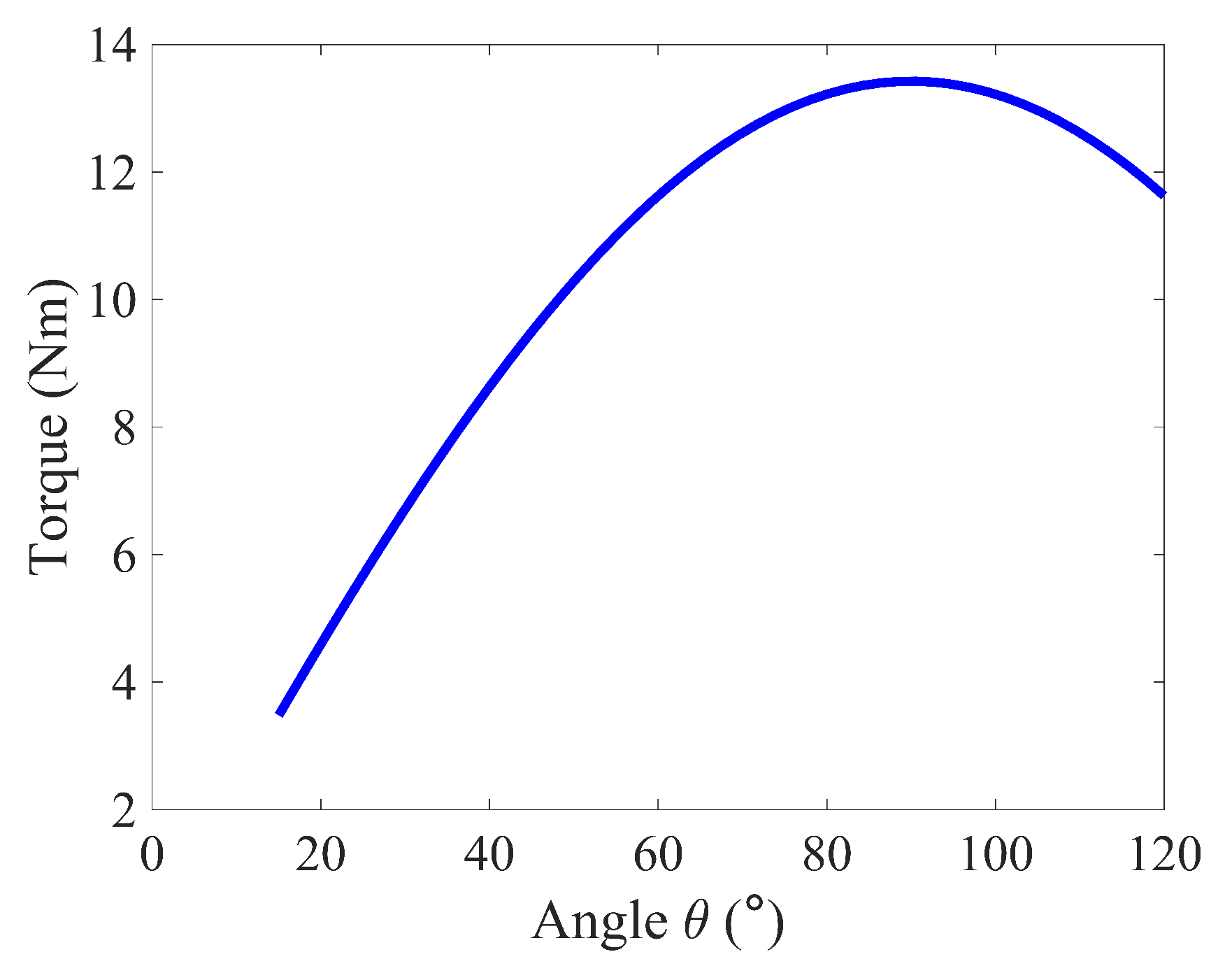
Figure 2 illustrates the torque required to rotate the elbow with a constant angular velocity from 15° of to 120° of flexion over 1.22 s . The torque increases with increasing elbow flexion until the arm reaches 90°, where the external load W becomes orthogonal to the forearm. The torque then decreases as the joint rotates past 90° to its final position as expected.

3.2. Muscle Forces

This subsection evaluates muscle forces during elbow flexion in three muscle models, highlighting the impact of small changes in tendon length. We start with the Simple Force Model, assessing basic force generation, then advance to the Hill-Type Active Model which integrates active force–length relationships, highlighting how slight tendon variations affect muscle dynamics. Finally, the Hill-Type Active and Passive Model incorporates passive properties, demonstrating detailed effects of tendon adjustments on overall muscle force accuracy.

3.2.1. Simple Force Model

By disregarding the constraints on muscle force generation imposed by the physiological force–length relationship, the Simple Force Model assumes that each muscle is capable of producing as much force as is necessary to drive the joint throughout the full range of elbow flexion. Therefore, the Simple Force Model allows us to assess how the choice of cost function exclusively influences the muscle force distribution. In particular it reveals that the choice of cost function significantly influences the distribution of muscle forces in biomechanical simulations as described below.
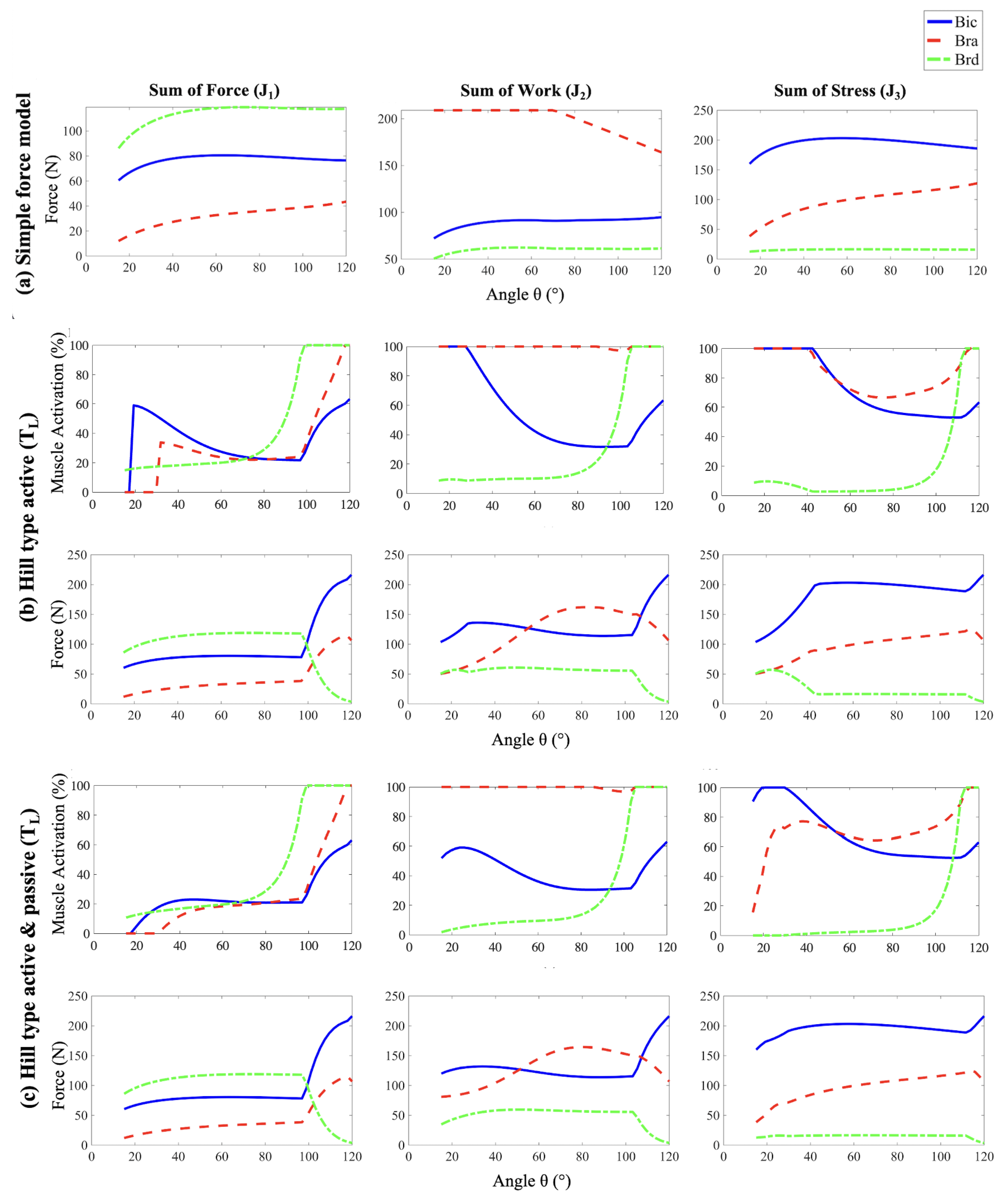
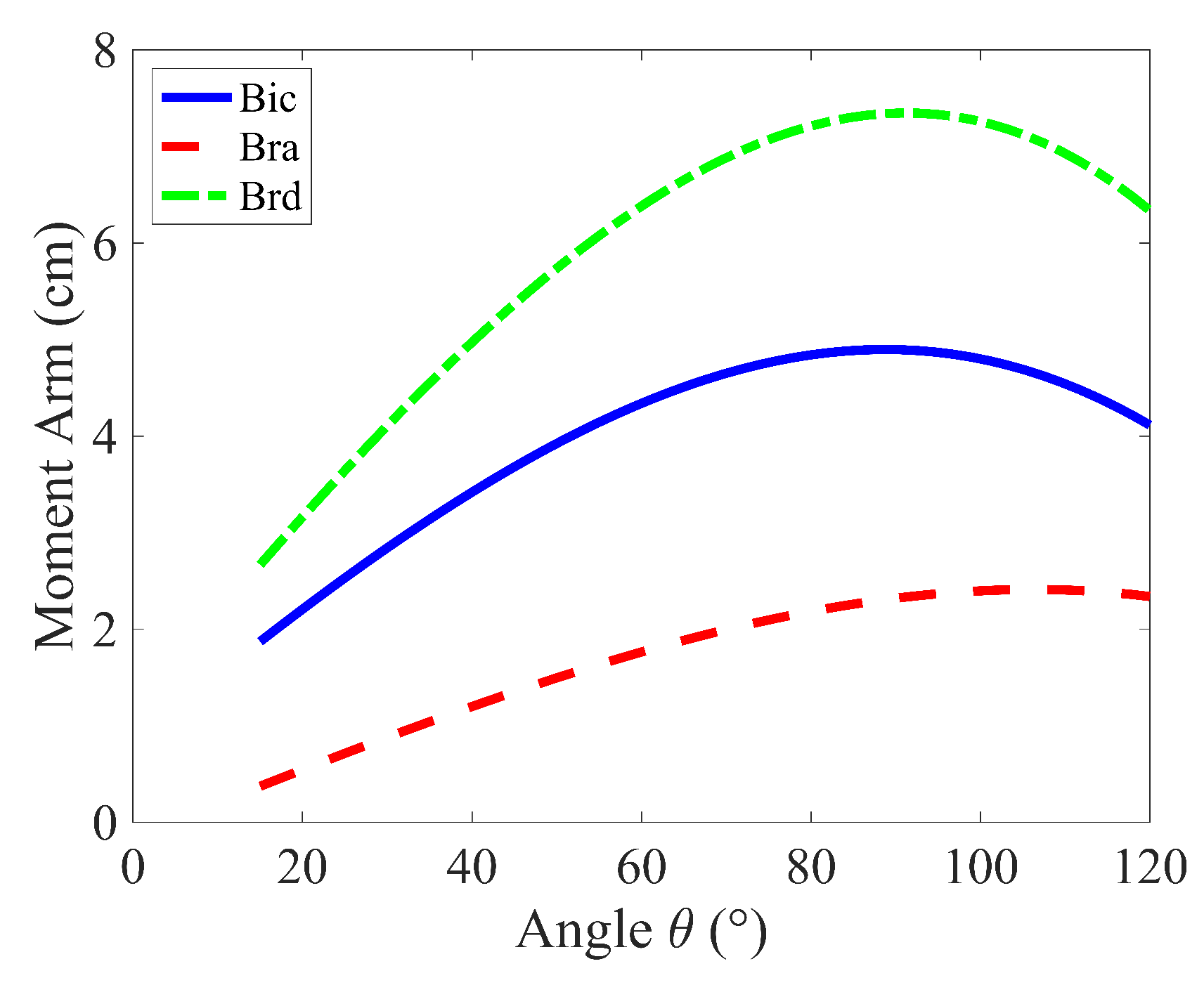
The results of the Simple Force Model, as shown in Figure 3a, indicate that minimizing the Sum of Forces (cost function J 1 ), the brachioradialis (brd) produces the largest forces, followed by the biceps brachii (bic), and then the brachialis (bra). Figure 4 illustrates that these force magnitudes are directly related to their respective moment arms. This outcome is predictable because muscles with longer moment arms have a mechanical advantage in generating torque. Consequently, these muscles tend to bear a larger share of the load, as increasing force in muscles with shorter moment arms contributes less effectively to the overall torque, making them less efficient in terms of torque production.
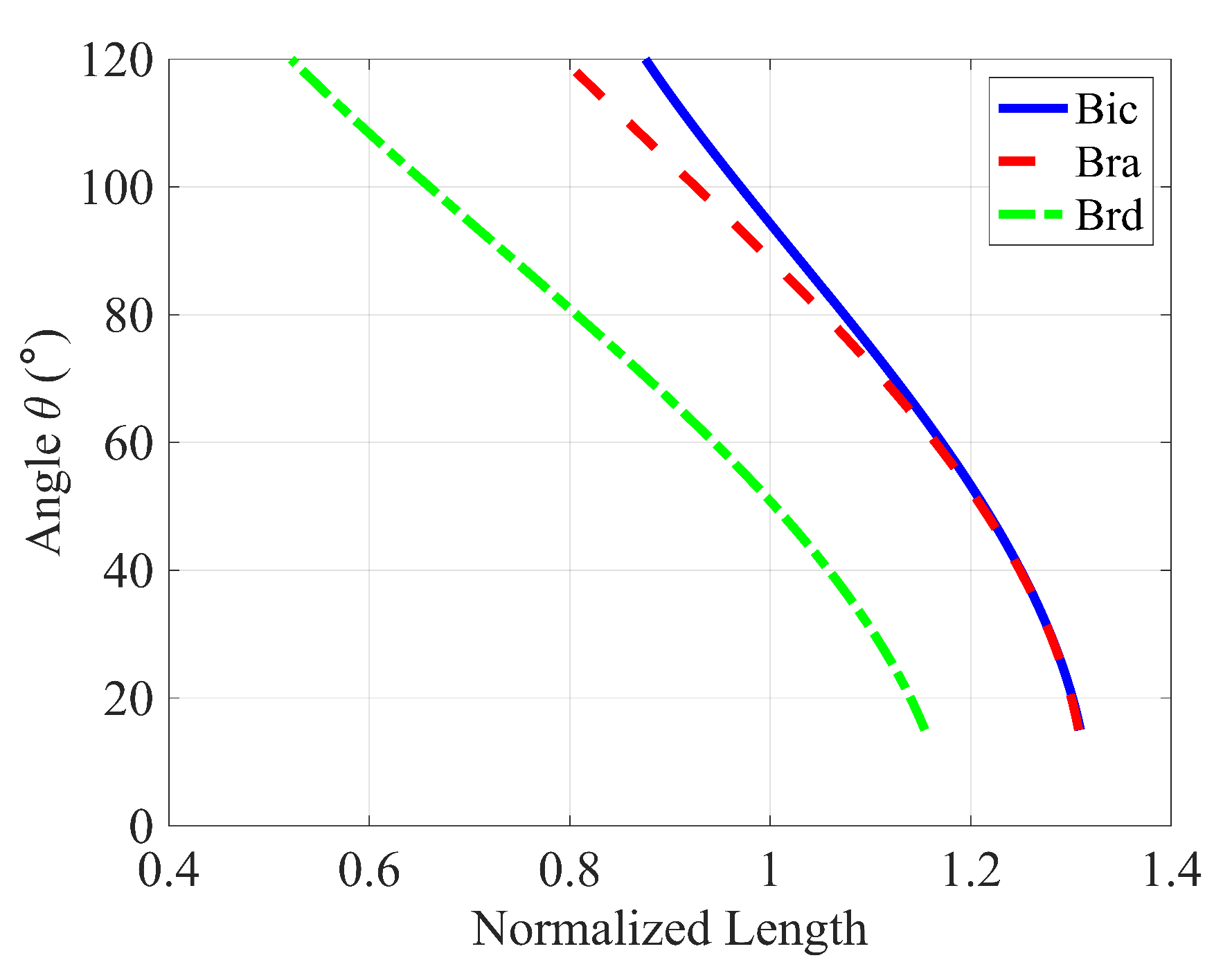
The Sum of Work cost function ( J 2 ) aims to minimize the total mechanical work done by the muscles. Given that work is the product of force and the muscle’s change in length, muscles that change length less will need to exert more force. This function shows how biomechanical efficiency can be modeled and optimized by balancing force output against changes in muscle length. Among the three muscle groups, bra is the shortest, and so is the change in its length during flexion, followed by bic and brd. Hence, as seen in Figure 3a, bra exerts the greatest force, with bic next, and brd exerting the least.
The Sum of Stress cost function ( J 3 ) aims to minimize total stress, where the stress in each muscle is defined as the force exerted by it per unit of physiological cross-sectional area (PCSA) of the muscle. Muscles with larger PCSAs can therefore sustain higher forces. This cost function is particularly useful for understanding how structural muscle properties like PCSA influence the biomechanical performance and force capabilities of different muscles. Among the three muscle groups, bra has the largest PCSA ( 5.6 cm 2 ), closely followed by bic ( 5.1 cm 2 ), and brd ( 1.2 cm 2 ) [37,38]. Since the PCSA for bra and bic are comparable, the muscle with the longest moment arm, bic, is leveraged to exert the highest force, followed by bra, and brd, as shown in Figure 3a.
Overall, using the Simple Force Model to evaluate these cost functions illustrates how each function impacts muscle force predictions differently based on mechanical and physiological principles.

3.2.2. Hill-Type Active

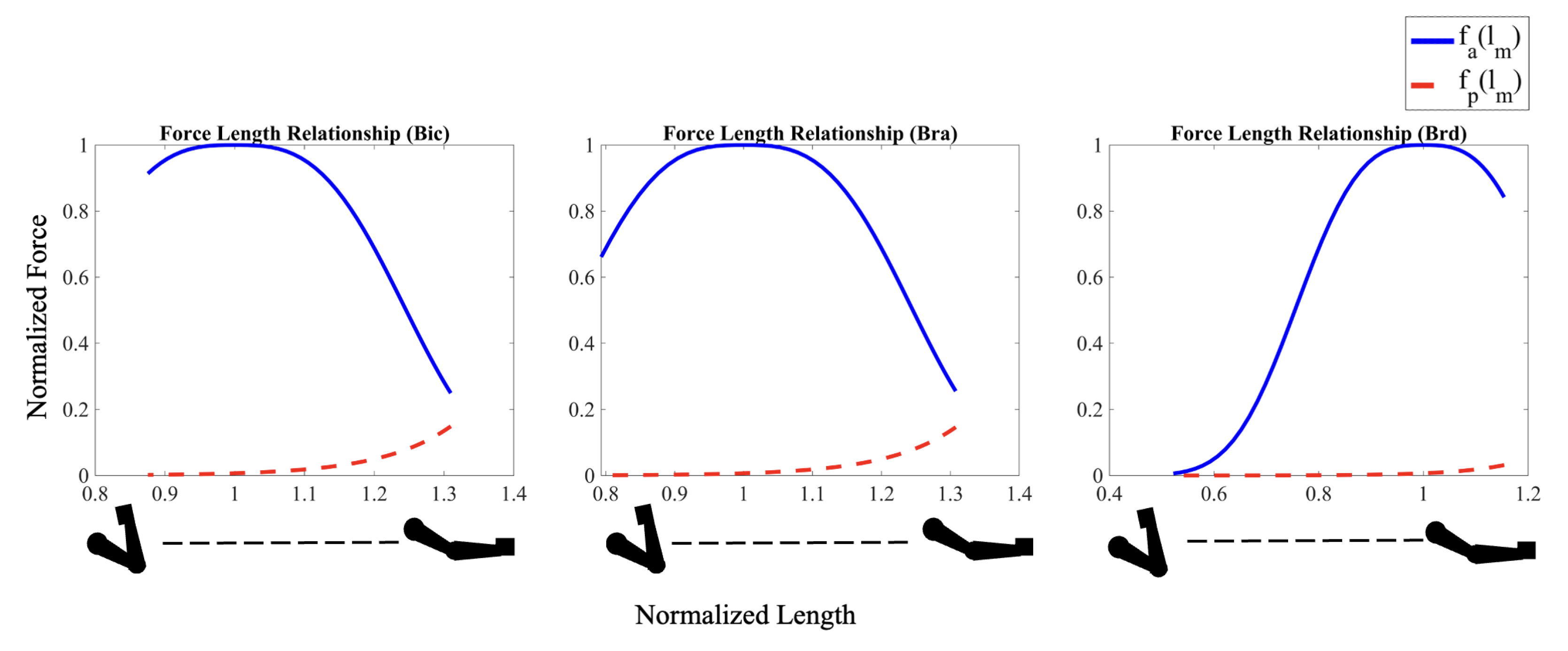
The addition of the active force–length relationship of skeletal muscle to the model introduces a physiologically relevant limit on the maximum force that each muscle can exert during contraction. As seen in Figure 5, when accounting for the force–length relationship for each muscle, the bic, bra, and brd can produce maximum active force at approximately 95°, 90°, and 50° of elbow flexion, respectively. As muscle length shortens (higher flexion angles) or lengthens (lower flexion angles) relative to this optimum length, the maximum possible force that each muscle can produce decreases accordingly (Figure 6). For small flexion angles, the limits on maximum force production are much more pronounced for the bic and bra muscles than for the brd.
Indeed, when compared to the Simple Force model, the forces produced at the start of each Hill-type active simulation are significantly lower for the bic and bra muscles for all three cost functions, despite both muscles exhibiting relatively high levels of activation. These effects are particularly pronounced for the Sum of Work and Sum of Stress cost functions, where the bic and bra muscles are at maximum activation as shown in Figure 3b. On the contrary, the brd forces are higher than predicted by the cost functions alone at these angles even while experiencing less than 20 % activation.
The effects of force–length relationships on muscle recruitment continue throughout the curling motion. As the flexion angle approaches the 90° where the bic and bra are nearer their optimal length, their force production increases even as their activation level decreases. At the same time, the brd shortens past its optimal length so that its force-producing capabilities drastically decrease. As such, the brd rapidly approaches maximum activation, its force production levels, and eventually drops. The sudden decrease in brd force production coincides with rapid increases in bic and bra force production as they approach their optimal length, and the applied moment about the elbow reaches a maximum.

3.2.3. Hill-Type Active and Passive

The passive force-length relationship further tunes the initial results by including additional force potential in the fully extended arm position, similar to an extended spring, as shown in Figure 6. The addition of the passive force–length relationship of each muscle plays an important role in muscle forces and activation, especially as the stretch ratios moves beyond 1.1 . When the arm is in a fully extended position, all three muscles are in a stretched configuration that generates large passive forces seeking to contract the muscle. The passive component exponentially decrease to low values as the muscles approach their optimum length. The addition of this passive force changes the total force trends exhibited by the bic and bra muscles, increasing the forces produced for the sum of work and the sum of stress cost functions, where these muscle forces dominate (Figure 3c). Similarly, the decrease in muscle activation of the bic and bra muscles at small flexion angles is partially due to the large passive restoring forces at these angles. Once each muscle has shortened past its optimum length, where the passive force component approaches zero (Figure 6) the force and muscle activation trends become similar to the active-only model. The inclusion of both active and passive components allows the model to capture the complex, nonlinear behavior of muscles, which became the deliberate choice for further analysis and validation.

3.3. Model Validation

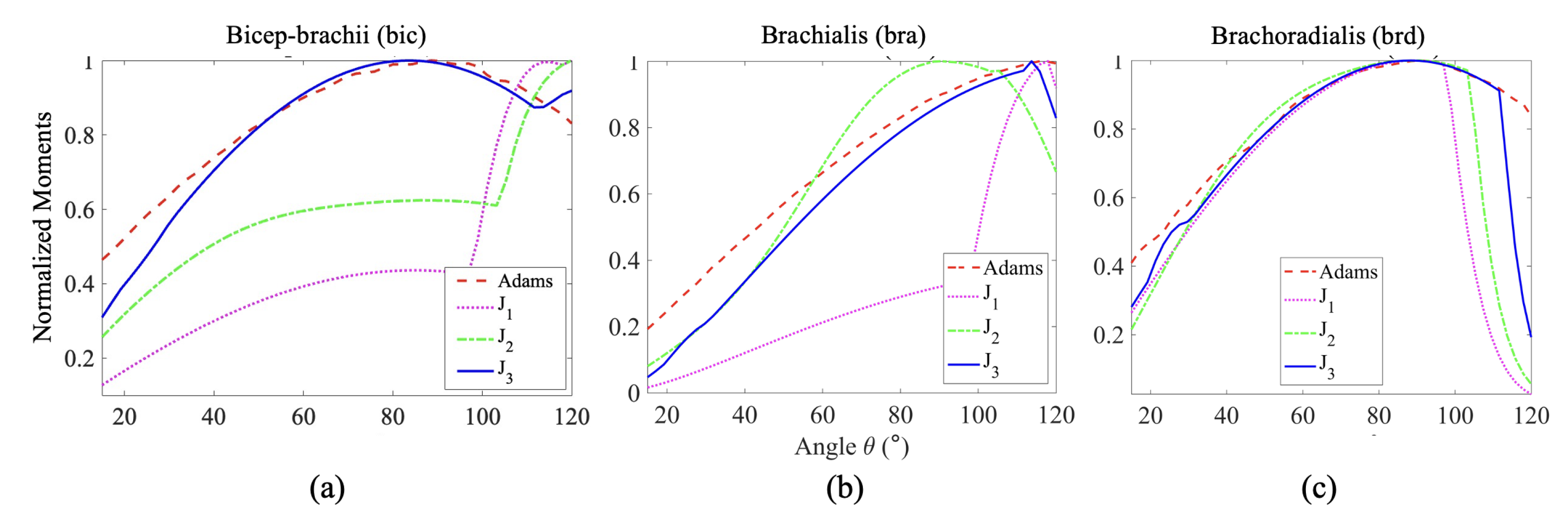
The comparisons between the normalized moment arm data Figure 7 reveal a similar trend of change in moment arm for each muscle with respect to the angle of elbow flexion. The normalized moment arm for the three elbow flexors gradually increases to its maximum, around 90° where the moment is at its peak, then decreases. We suspect that the slight variation arose from the variation of muscle length, PCSA value, muscle placement, and relative orientation among the individual subjects taken into account from the literature. In Figure 8c, the energy cost function ( J 1 ) , the work cost function ( J 2 ) and the stress cost function ( J 3 ) provide normalized moments that align well with the observed moments for the brd muscle. For the bra muscle (Figure 8b), the work and stress cost functions show fewer deviations from the results in [42] compared to the force criterion. Regarding the estimation of muscle moment, the stress cost function for the bic muscle (Figure 8a) appears to show the closest agreement with the findings in [42].
It is worth noting that the stress cost function captures the increasing trend of the muscle moment with greater accuracy for all the muscles. This observation is quantified in Table 3 with the Mean Squared Errors calculated with respect to the muscle moments (red dashed curves in Figure 8) computed using MSE ADAMS 2010 [42]. The stress cost function ( J 3 ) has the least mean squared error for the bicep and brachoradialis, while the work cost function ( J 2 ) has the least error for the brachialis muscle. The mean squared error of J 3 is the least, second to J 2 for Brachialis.

4. Discussion

Our analysis revealed that all three simple cost functions are reasonably accurate in estimating muscle forces for brachioradialis, while for brachialis, the work and stress cost functions gave a fair estimate and the stress cost function provided a fitting estimate for the bicep. Overall, the combination of stress cost function along with the Hill-type muscle model with active and passive force length relationship provides the most reliable estimation of muscle forces for the three muscle groups during an elbow flexion. This simple cost function sensibly captures the increase in muscle force to its peak. The deviations observed beyond the peaks can be attributed to variations in the task configurations and the estimated muscle parameters for different subjects. The trend of increasing muscle force is an essential muscle behavior, and its estimation can be beneficial in the aforementioned domains where accurate force measurements are not the primary focus, such as performance evaluation, injury prevention, muscle activation assessment, etc.
Our approach focuses on achieving a delicate balance between accuracy and usability, acknowledging that the pursuit of the utmost precision is not always paramount. This equilibrium drives us to explore scenarios where a reasonable level of accuracy suffices without necessitating the use of highly complex models. This balance or trade-off is useful in situations where incorporating EMG data could introduce complexity or when these data are simply not accessible. Furthermore, because this approach to muscle force estimation obviates the need for intricate EMG data, it not only simplifies exploration with various combinations of muscle models and cost functions but also allows for easier customization to accommodate a diverse range of demographics and populations, encompassing different age groups, genders, and health conditions. This ease of exploration and customization holds significant value in practical applications where a detailed biomechanical analysis may not be the primary focus, making the integration of muscle force estimation readily feasible in such scenarios. For example: (a) Physical Therapy and Rehabilitation monitoring, where the primary goal may be to monitor patient progress and track changes in muscle activation rather than achieving precise muscle force estimation; (b) Exploratory studies of biomechanical research, specifically while developing new methodologies for muscle activation patterns and trends exploration; (c) Athletic Training and Performance Assessment, where the focus may be on performance assessment, movement optimization, and injury prevention, and (d) Basic Physiology and Exercise Science. In future work, this study can be extended to formulate models for other body segments or joints and for different motions, such as knee extensions, abduction, adduction, rotation, etc.

5. Conclusions

This study demonstrates that the use of simple cost functions does not significantly compromise the accuracy of muscle force estimates, provided that they are combined with a sufficiently representative muscle model. The choice of the physiological muscle model is more important than the cost function since a more accurate muscle model captures the nonlinear behavior of the muscle, and the cost function provides an optimal strategy. Relatively simple mathematical cost functions can drive muscle force optimization and capture the essential aspects of muscle behavior, excluding the requirement for EMG data. This approach is highly beneficial in cases where the respective EMG data are simply not accessible. It can be effective and favorable for estimating the behavior of deep muscles, as EMG data for these muscles are difficult to obtain and prone to measurement errors. Furthermore, separately considering the cost function optimization and the muscle model allows for evaluation of their impact independently on the forces estimation as well as their combined effects.

Author Contributions

Conceptualization, M.L. and S.G.; methodology, M.H.A., J.-E.N. and R.D.; software, M.H.A., J.-E.N. and R.D.; validation, M.H.A., J.-E.N. and R.D.; formal analysis, M.H.A., J.-E.N., R.D., M.L. and S.G.; investigation, M.H.A., J.-E.N., R.D., M.L. and S.G.; data curation, M.H.A., J.-E.N. and R.D.; validation, M.H.A., J.-E.N. and R.D.; writing—original draft preparation, M.H.A.; writing—review and editing, M.H.A., J.-E.N., R.D., M.L. and S.G.; visualization, M.H.A., J.-E.N., R.D., M.L. and S.G.; supervision, M.L. and S.G.; project administration, M.L. and S.G.; funding acquisition, S.G. All authors have read and agreed to the published version of the manuscript.

Funding

This research received no external funding.

Institutional Review Board Statement

Not applicable.

Informed Consent Statement

Not applicable.

Data Availability Statement

The data presented in this study are available on request from the corresponding author.

Acknowledgments

During the preparation of this work the author(s) used OpenAI-ChatGPT to grammar check, simplify and improve readability and language for the reader. After using this tool, the authors reviewed and edited the content as needed, and take full responsibility for the content of the publication.

Conflicts of Interest

Matthew Leineweber was employed by Biomotum. The remaining authors declare that the research was conducted in the absence of any commercial or financial relationships that could be construed as a potential conflict of interest.

Abbreviations

The following abbreviations are used in this manuscript:
bicbiceps brachii
brabrachialis
brdbrachoradialis
DoFdegrees of freedom
EMGelectromyography
PCSAphysiological cross-sectional area

References

  1. Serrancolí, G.; Font-Llagunes, J.M.; Barjau, A. A weighted cost function to deal with the muscle force sharing problem in injured subjects: A single case study. J. Multi-Body Dyn. 2014, 228, 241–251. [Google Scholar] [CrossRef]
  2. Silva, M.T.; Ambrósio, J.A. Solution of redundant muscle forces in human locomotion with multibody dynamics and optimization tools. Mech. Based Des. Struct. Mach. 2003, 31, 381–411. [Google Scholar] [CrossRef]
  3. Nikooyan, A.A.; Veeger, H.E.J.; Chadwick, E.K.J.; Praagman, M.; van der Helm, F.C.T. Development of a comprehensive musculoskeletal model of the shoulder and elbow. Med. Biol. Eng. Comput. 2011, 49, 1425–1435. [Google Scholar] [CrossRef] [PubMed]
  4. Paraschiv, C.; Paraschiv, P.; Cimpoeşu, R. Determination of the elbow joint resulting torque and obtaining customized numerical results. Procedia 2014, 117, 522–528. [Google Scholar] [CrossRef]
  5. Robertson, G.; Caldwell, G.; Hamill, J.; Kamen, G.; Whittlesey, S. Research Methods in Biomechanics, 2nd ed.; Human Kinetics: Champaign, IL, USA, 2013. [Google Scholar]
  6. Erdemir, A.; McLean, S.; Herzog, W.; van den Bogert, A.J. Model-based estimation of muscle forces exerted during movements. Clin. Biomech. 2007, 22, 131–154. [Google Scholar] [CrossRef]
  7. Tsirakos, D.; Baltzopoulos, V.; Bartlett, R. Inverse optimization: Functional and physiological considerations related to the force-sharing problem. Crit. Rev. Biomed. Eng. 1997, 25, 371–407. [Google Scholar] [CrossRef]
  8. Zonnino, A.; Sergi, F. Model-based estimation of individual muscle force based on measurements of muscle activity in forearm muscles during isometric tasks. IEEE Trans. Biomed. Eng. 2019, 1, 171. [Google Scholar] [CrossRef]
  9. Shourijeh, M.S.; Fregly, B.J. Muscle synergies modify optimization estimates of joint stiffness during walking. J. Biomech. Eng. 2020, 142, 310. [Google Scholar] [CrossRef]
  10. Ao, D.; Shourijeh, M.S.; Patten, C.; Fregly, B.J. Evaluation of Synergy Extrapolation for Predicting Unmeasured Muscle Excitations from Measured Muscle Synergies. Front. Comput. Neurosci. 2020, 14, 588943. [Google Scholar] [CrossRef]
  11. Hardt, D. Determining muscle forces in the leg during normal human walking—An application and evaluation of optimization methods. J. Biomech. Eng. 1978, 100, 72–78. [Google Scholar] [CrossRef]
  12. Crowninshield, R.D.; Brand, R.A. A physiologically based criterion of muscle force prediction in locomotion. J. Biomech. 1981, 14, 793–801. [Google Scholar] [CrossRef] [PubMed]
  13. Heintz, S.; Gutierrez-Farewik, E.M. Static optimization of muscle forces during gait in comparison to EMG-to-force processing approach. Gait Posture 2007, 26, 279–288. [Google Scholar] [CrossRef] [PubMed]
  14. Zajac, F. Muscle and tendon: Properties, models, scaling, and application to biomechanics and motor control. Crit. Rev. Biomed. Eng. 1989, 17, 359–411. [Google Scholar] [PubMed]
  15. Lai, A.K.M.; Biewener, A.A.; Wakeling, J.M. Metabolic cost underlies task-dependent variations in motor unit recruitment. J. R. Soc. Interface 2018, 15, 20180541. [Google Scholar] [CrossRef] [PubMed]
  16. Ting, L.H.; Chvatal, S.A.; Safavynia, S.A.; McKay, J.L. Review and perspective: Neuromechanical considerations for predicting muscle activation patterns for movement. Int. J. Numer. Methods Biomed. Eng. 2012, 28, 1003–1014. [Google Scholar] [CrossRef]
  17. Michaud, F.; Lamas, M.; Lugrís, U.; Cuadrado, J. A fair and EMG-validated comparison of recruitment criteria, musculotendon models and muscle coordination strategies, for the inverse-dynamics based optimization of muscle forces during gait. J. Neuroeng. Rehabil. 2020, 18, 17. [Google Scholar] [CrossRef]
  18. Wena, J.; Raison, M.; Achiche, S. Using a cost function based on kinematics and electromyographic data to quantify muscle forces. J. Biomech. 2018, 80, 151–158. [Google Scholar] [CrossRef]
  19. Seireg, A.; Arvikar, R. A mathematical model for evaluation of forces in lower extremeties of the musculo-skeletal system. J. Biomech. 1973, 6, 313–326. [Google Scholar] [CrossRef]
  20. Penrod, D.; Davy, D.; Singh, D. An optimization approach to tendon force analysis. J. Biomech. 1974, 7, 123–129. [Google Scholar] [CrossRef]
  21. Crowninshield, R.D.; Johnston, R.C.; Andrews, J.G.; Brand, R.A. A biomechanical investigation of the human hip. J. Biomech. 1978, 11, 75–85. [Google Scholar] [CrossRef]
  22. Dul, J.; Johnson, G.; Shiavi, R.; Townsend, M. Muscular synergism—II. A minimum-fatigue criterion for load sharing between synergistic muscles. J. Biomech. 1984, 17, 675–684. [Google Scholar] [CrossRef] [PubMed]
  23. Racinais, S.; Maffiuletti, N.A.; Girard, O. M-wave, H- and V-reflex recruitment curves during maximal voluntary contraction. J. Clin. Neurophysiol. 2013, 30, 415–421. [Google Scholar] [CrossRef] [PubMed]
  24. Sartori, M.; Farina, D.; Lloyd, D.G. Hybrid neuromusculoskeletal modeling to best track joint moments using a balance between muscle excitations derived from electromyograms and optimization. J. Biomech. 2014, 47, 3613–3621. [Google Scholar] [CrossRef] [PubMed]
  25. Buchanan, T.S.; Lloyd, D.G.; Manal, K.; Besier, T.F. Neuromusculoskeletal modeling: Estimation of muscle forces and joint moments and movements from measurements of neural command. J. Appl. Biomech. 2004, 20, 367–395. [Google Scholar] [CrossRef]
  26. Praagmana, M.; Chadwickb, E.; van der Helmb, F.; Veegera, H. The relationship between two different mechanical cost functions and muscle oxygen consumption. J. Biomech. 2006, 39, 758–765. [Google Scholar] [CrossRef]
  27. Veerkamp, K.; Waterval, N.; Geijtenbeek, T.; Carty, C.; Lloyd, D.; Harlaar, J.; van der Krogt, M. Evaluating cost function criteria in predicting healthy gait. J. Biomech. 2021, 123, 110530. [Google Scholar] [CrossRef]
  28. Islam, S.U.; Glover, A.; MacFarlane, R.J.; Mehta, N.; Waseem, M. The Anatomy and Biomechanics of the Elbow. Open Orthop. J. 2020, 14, 95–99. [Google Scholar] [CrossRef]
  29. Malagelada, F.; Dalmau-Pastor, M.; Vega, J.; Golanó, P. Elbow Anatomy. Sport. Inj. 2014, 2, 527–553. [Google Scholar]
  30. Ettema, G.; Styles, G.; Kippers, V. The moment arms of 23 muscle segments of the upper limb with varying elbow and forearm positions: Implications for motor control. Hum. Mov. Sci. 1998, 17, 201–220. [Google Scholar] [CrossRef]
  31. Mitiguy, P. Dynamics of Mechanical, Aerospace, & Bio/Robotic Systems. Available online: http://www.motiongenesis.com (accessed on 13 September 2024).
  32. Nikravesh, P.E. Computer-Aided Analysis of Mechanical Systems; Prentice-Hall, Inc.: Hoboken, NJ, USA, 1988. [Google Scholar]
  33. Wendlova, J. Why is so important to balance the muscular dysbalance in mm. coxae area in osteoporotic patients? Bratisl. Lekárske Listy 2008, 109, 502–507. [Google Scholar]
  34. Maso, F.D.; Begon, M.; Raison, M. Methodology to customize maximal isometric forces for hill-type muscle models. J. Appl. Biomech. 2016, 33, 80–86. [Google Scholar] [CrossRef] [PubMed]
  35. Jo, S. A computational neuromusculoskeletal model of human arm movements. Int. J. Control. Autom. Syst. 2011, 9, 913–923. [Google Scholar] [CrossRef]
  36. Chang, Y.W.; Su, F.C.; Wu, H.W.; An, K.N. Optimum length of muscle contraction. Clin. Biomech. 1999, 14, 537–542. [Google Scholar] [CrossRef] [PubMed]
  37. Lemay, M.A.; Crago, P.E. A Dynamic Model for Simulating Movements of the Elbow, Forearm, and Wrist. J. Biomech. 1990, 29, 1319–1330. [Google Scholar] [CrossRef]
  38. Murray, W.M.; Buchanan, T.S.; Delp, S.L. The isometric functional capacity of muscles that cross the elbow. J. Biomech. 2000, 33, 943–952. [Google Scholar] [CrossRef]
  39. MathWorks. lsqlin—Solve Linear Least-Squares Problems with Linear Constraints. Available online: https://www.mathworks.com/help/optim/ug/lsqlin.html (accessed on 13 September 2024).
  40. MathWorks. fmincon—Find the Minimum of a Constrained Nonlinear Multivariable Function. Available online: https://www.mathworks.com/help/optim/ug/fmincon.html (accessed on 13 September 2024).
  41. Murray, W.M.; Delp, S.L.; Buchanan, T.S. Variation of muscle moment arms with elbow and forearm position. J. Biomech. 1995, 28, 513–525. [Google Scholar] [CrossRef]
  42. Ilbeigi, S.; Ramezani, H. Assessment and modelling of elbow joint for analysing of muscle moment and reaction force during flexion movement with ADAMS Software. Eur. J. Sport. Exerc. Sci. 2014, 3, 18–26. [Google Scholar]
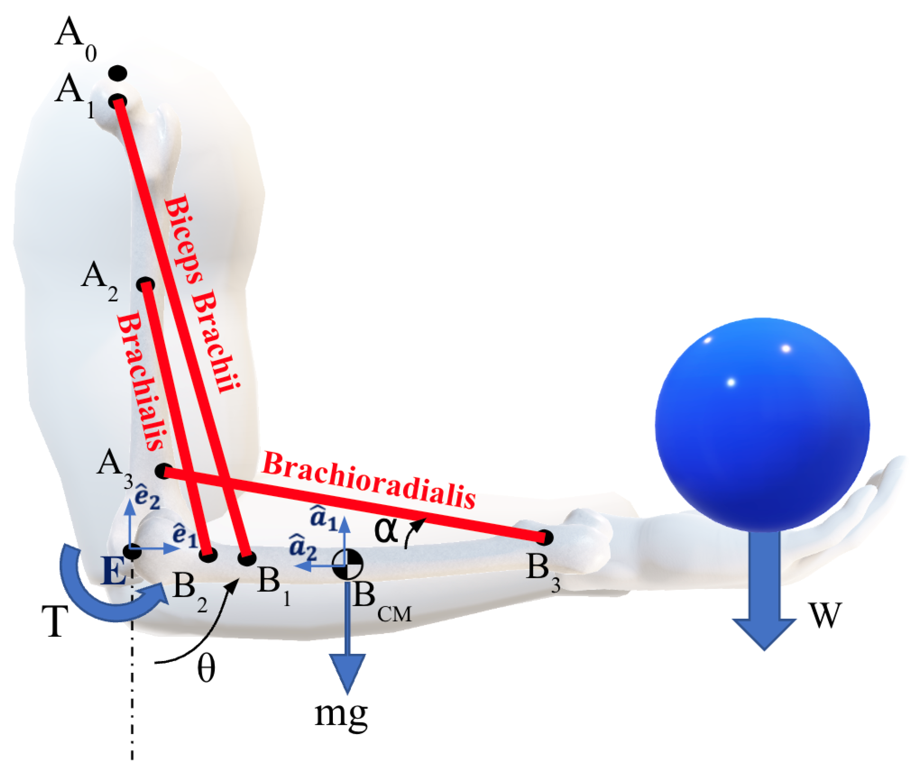
Figure 1. Flexion of the elbow joint is actuated by the group of three muscles: Biceps brachii, brachialis, and brachoradialis.
Biomed 04 00028 g001
Figure 2. Elbow joint torque during curl ( 15 ° θ 120 ° ).
Biomed 04 00028 g002
Figure 3. The forces exerted by the three muscle groups (bic, bra and brd) on the forearm as a function of angle of flexion as estimated by employing three different muscle models (ac) along with the three cost functions J 1 , J 2 and J 3 (arranged column-wise). For the two Hill-type models (b,c), the muscle activations are also shown. T L refers to linear tendon length change approximation.
Biomed 04 00028 g003
Figure 4. Moment arm variation of muscles groups during the curling motion ( 15 ° θ 120 ° ).
Biomed 04 00028 g004
Figure 5. Variations in normalized muscle lengths during the elbow curl.
Biomed 04 00028 g005
Figure 6. Force Length Relationship (both active and passive) for the arm muscles as a function of their stretch ratio. Both active ( f a ( l m ) ) and passive ( f p ( l m ) ) forces are normalized by the maximum isometric force at optimal length for each muscle. Normalized lengths for each muscle are expressed relative to its optimum length.
Biomed 04 00028 g006
Figure 7. Comparison of Estimated Normalized Moment arm of (a) Bicep, (b) Brachialis and (c) Brachoradialis for an Elbow flexion with the calculated moments by Wendy et al. [41] for a male and female subject and with their 3D-Computer model.
Biomed 04 00028 g007
Figure 8. Normalized moment plots of (a) Biceps, (b) Brachialis and (c) Brachoradialis muscles, obtained from the three optimization techniques, J 1 (Force criterion), J 2 (Work criterion) and J 3 (Stress criterion), considering Hill-Type Active and Passive muscle model, compared with muscle moments obtained from a computational model using ADAMS Software by Ilbeigi et al. [42].
Biomed 04 00028 g008
Table 1. Dimensions, Forearm Inertial Properties and Muscle Origin and Insertion Points.
Humerus Length ( A 0 E ),  L H   ( cm ) 29
Forearm Length ( EB 3 ), L   ( cm ) 36
Forearm Center of Mass ( EB cm ),  L cg   ( cm )
(Distance from the Elbow Joint)
17.12
Forearm Mass, m   ( kg ) 1.53
Forearm Moment of Inertia, μ   ( kg · m 2 )
(About its Center of Mass)
7.04 × 10 3
Origin (at Humerus)Insertion (at Forearm)
bic ( cm ) 1.21 ( A 0 A 1 ) 4.84 ( E B 1 )
bra ( cm ) 17.39 ( A 0 A 2 ) 2.39 ( E B 2 )
brd ( cm ) 7.31 ( A 0 A 3 ) 36 ( E B 3 )
Table 2. List of cost-functions, to predict the individual muscle force.
Cost FunctionDescription
J 1 = F m , i 2 Sum of Force criterion
J 2 = F m , i Δ l m , i 2 Sum of Work criterion
J 3 = F m , i P C S A m , i 2 Sum of Stress criterion
F m , i : magnitude of force exerted by the ith muscle; Δ l m , i : change in length of the ith muscle; P C S A m , i : physiological cross-sectional area of the ith muscle.
Table 3. Statistical Analysis of the Plots.
Mean Squared Error
Muscle J 1 J 2 J 3
Bicep0.19260.07920.0029
Brachialis0.16120.01470.0089
Brachoradialis0.09890.06450.0207
Disclaimer/Publisher’s Note: The statements, opinions and data contained in all publications are solely those of the individual author(s) and contributor(s) and not of MDPI and/or the editor(s). MDPI and/or the editor(s) disclaim responsibility for any injury to people or property resulting from any ideas, methods, instructions or products referred to in the content.