
Data Structures for 2D Representation of Terrain Models


Definition
1. Introduction
2. Surface Representation
2.1. Raster
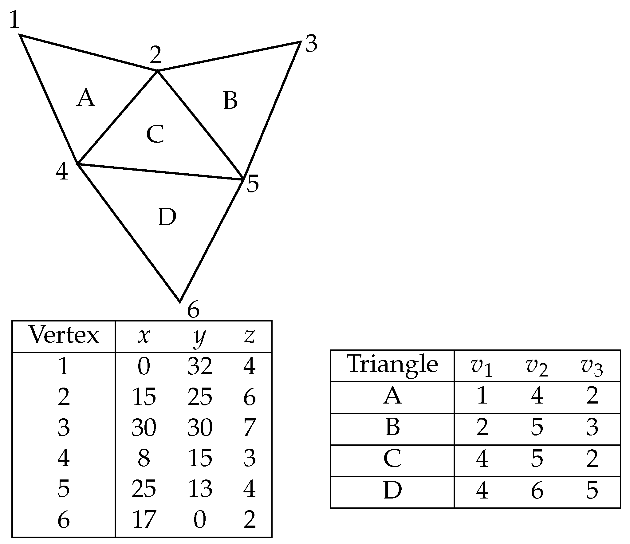
2.2. TIN
2.3. Hexagonal Grid
3. Morphological Structures
3.1. Contour Graphs and Trees
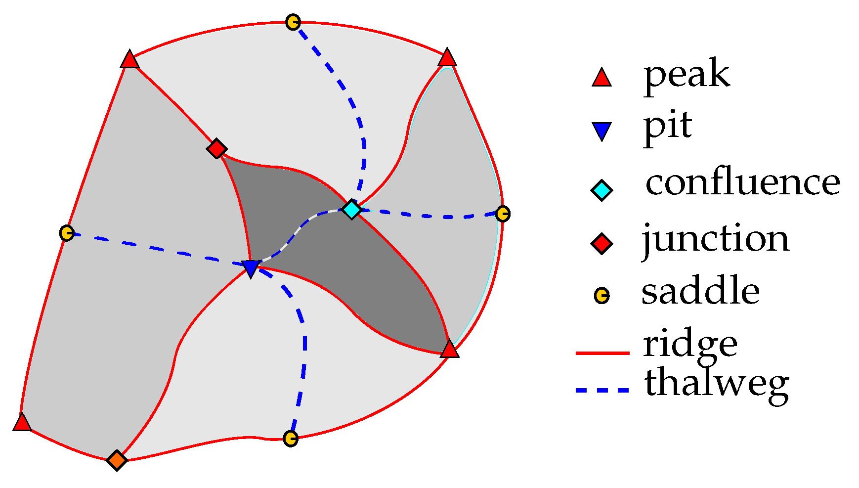
3.2. Surface Networks
- A ridge connects a peak and a saddle;
- A thalweg connects a pit and a saddle;
- Ridges and thalwegs intersect only at saddles;
- At a saddle, the number of ridges is equal to the number of thalwegs;
- When turning around a saddle, edges alternate between ridges and thalwegs.
3.3. Extended Surface Networks
3.4. The Cognitive Use of Extended Surface Networks
4. Conclusions
Author Contributions
Funding
Data Availability Statement
Conflicts of Interest
References
- Morato-Moreno, M. Orígenes de la representación topográfica del terreno en algunos mapas hispanoamericanos del siglo XVI. Boletín Asoc. Geógrafos Españoles 2017, 73, 175–199. [Google Scholar] [CrossRef]
- Miller, C.L.; Laflamme, R.A. The Digital Terrain Model - Theory and Application. Photogramm. Eng. 1958, XXIV, 433–442. [Google Scholar]
- Li, Z.; Zhu, Q.; Gold, C. Digital Terrain Modeling, Principles and Methodology; CRC Press: Boca Raton, FL, USA, 2005. [Google Scholar]
- Dikau, R. The application of a digital relief model to landform analysis. In Three Dimensional Applications in Geographical Information Systems; Raper, J., Ed.; Taylor & Francis: London, UK, 1989; pp. 51–77. [Google Scholar]
- Blaschke, T. Object based image analysis for remote sensing. ISPRS J. Photogramm. Remote Sens. 2010, 65, 2–16. [Google Scholar] [CrossRef]
- Thibault, D.; Gold, C. Terrain Reconstruction from Contours by Skeleton Construction. GeoInformatica 2000, 4, 349–373. [Google Scholar] [CrossRef]
- Hutchinson, M. A new method for gridding elevation and stream line data with automatic removal of spurious pits. J. Hydrol. 1989, 106, 211–232. [Google Scholar] [CrossRef]
- Choma, A.; Ratcliff, C.; Frisina, R. Evaluation of Remote Sensing Technologies for High-resolution Terrain Mapping. In Proceedings of the SSC 2005 Spatial Intelligence, Innovation and Praxis: The National Biennial Conference of the Spatial Sciences Institute, Spatial Sciences Institute, Melbourne, VA, Australia, 12–16 September 2005. [Google Scholar]
- Clarke, K.; Romero, B. On the topology of topography: A review. Cartogr. Geogr. Inf. Sci. 2016, 44, 271–282. [Google Scholar] [CrossRef]
- Lindsay, J.B. Efficient hybrid breaching-filling sink removal methods for flow path enforcement in digital elevation models. Hydrol. Processes 2016, 30, 846–857. [Google Scholar] [CrossRef]
- Peuquet, D.J. Representations of Space and Time; The Guilford Press: New York, NY, USA, 2002. [Google Scholar]
- Cayley, A. On Contour and Slope Lines. London Edinburgh Dublin Philos. Mag. J. Sci. 1859, 18, 264–268. [Google Scholar] [CrossRef]
- Maxwell, J.C. On Hills and Dales. Philos. Mag. Ser. 4 1870, 40, 421–427. [Google Scholar] [CrossRef]
- Pfaltz, J. Surface networks. Geogr. Anal. 1976, 8, 77–93. [Google Scholar] [CrossRef]
- Rana, S. (Ed.) Topological Data Structures for Surfaces. An Introduction to Geographical Information Science; Wiley: Chichester, UK, 2004. [Google Scholar]
- Deng, Y. New trends in digital terrain analysis: Landform definition, representation, and classification. Prog. Phys. Geogr. 2007, 31, 405–419. [Google Scholar] [CrossRef]
- Fisher, P.; Wood, J.; Cheng, T. Where is Helvellyn? Fuzziness of multi-scale landscape morphometry. Trans. Inst. Br. Geogr. 2004, 29, 106–128. [Google Scholar] [CrossRef]
- Kaba, J.; Peters, J. A pyramid-based approach to interactive terrain visualization. In Proceedings of the 1993 Symposium on Parallel Rendering, San Jose, CA, USA, 25–26 October 1993; pp. 67–70. [Google Scholar]
- Mark, D.M.; Lauzon, J.P.; Cebrian, J.A. A review of quadtree-based strategies for interfacing coverage data with digital elevation models in grid form. Int. J. Geogr. Inf. Syst. 1989, 3, 3–14. [Google Scholar] [CrossRef]
- Fowler, R.J.; Little, J.J. Automatic extraction of irregular network digital terrain models. ACM SIGGRAPH Comput. Graph. 1979, 13, 199–207. [Google Scholar] [CrossRef]
- Yvinec, M. 2D Triangulations. In CGAL User and Reference Manual, CGAL Editorial Board, 6.1 ed.; GeometryFactory: Antibes, France, 2024; Available online: https://www.cs.tau.ac.il/~efif/doc_output10/Triangulation_2/index.html (accessed on 3 April 2025).
- Blandford, D.K.; Blelloch, G.E.; Cardoze, D.E.; Kadow, C. Compact representations of simplicial meshes in two and three dimensions. Int. J. Comput. Geom. Appl. 2005, 15, 3–24. [Google Scholar] [CrossRef]
- Ledoux, H. startinpy: A Python library for modelling and processing 2.5D triangulated terrains. J. Open Source Softw. 2024, 9, 7123. [Google Scholar] [CrossRef]
- de Berg, M.; Cheong, O.; van Kreveld, M.; Overmars, M. Computational Geometry, Algorithms and Applications, 3rd ed.; Springer: Berlin/Heidelberg, Germany, 2008. [Google Scholar]
- Guibas, L.; Stolfi, J. Primitives for the manipulation of general subdivisions and the computation of Voronoi diagrams. ACM Trans. Graph. 1985, 4, 75–123. [Google Scholar] [CrossRef]
- Mioc, D.; Anton, F.; Gold, C.; Moulin, B. Reversibility of the Quad-Edge operations in the Voronoi data structure. In Proceedings of the International Symposium on Voronoi Diagrams in Science and Engineering (ISVD), Glamorgan, UK, 9–11 July 2007; pp. 135–144. [Google Scholar] [CrossRef]
- Saux, E.; Thibaud, R.; Li, K.J.; Kim, M.H. A New Approach for a Topographic Feature-Based Characterization of Digital Elevation Data. In Proceedings of the Twelfth ACM International Symposium on Advances in Geographic Information Systems, Washington, DC, USA, 12–13 November 2004; Pfoser, D., Cruz, I.F., Ronthaler, M., Eds.; ACM Press: New York, NY, USA, 2004; pp. 73–100. [Google Scholar]
- Jones, N. Watershed delineation with triangle-based terrain models. J. Hydraul. Eng. 1990, 116, 1232–1251. [Google Scholar] [CrossRef]
- Rennó de Azeredo Freitas, H.; da Costa Freitas, C.; Rosim, S.; de Freitas Oliveira, J.R. Drainage networks and watersheds delineation derived from TIN-based digital elevation models. Comput. Geosci. 2016, 92, 21–37. [Google Scholar] [CrossRef]
- Tse, O.C.; Gold, C. Integration of Terrain Models and Built-Up Structures using CAD-Type Euler Operators. In Proceedings of the International Archives of the Photogrammetry, Remote Sensing and Spatial Information Sciences, Ottawa, ON, Canada, 9–12 July 2002; ISPRS: Paris, France, 2002; Volume XXXIV-5/W3. [Google Scholar]
- Lindstrom, P.; Koller, D.; Ribarsky, W.; Hodges, L.F.; Faust, N.; Turner, G.A. Real-time, continuous level of detail rendering of height fields. In Proceedings of the SIGGRAPH ’96, New Orleans, LA, USA, 4–9 August 1996; pp. 109–118. [Google Scholar]
- Schön, B.; Bertolotto, M.; Laefer, D.; Morrish, S. Storage, Manipulation, and Visualization of LiDAR Data. In Proceedings of the 3rd ISPRS International Workshop 3D-ARCH 2009: “3D Virtual Reconstruction and Visualization of Complex Architectures”, Trento, Italy, 25–28 February 2009; ISPRS: Paris, France, 2009; Volume XXXVIII-5/W1. [Google Scholar]
- Fellegara, R.; Iuricich, F.; De Floriani, L. Efficient representation and analysis of triangulated terrains. In Proceedings of the 25th ACM SIGSPATIAL International Conference on Advances in Geographic Information Systems (SIGSPATIAL ’17), Redondo Beach, CA, USA, 7–10 November 2017; ACM: New York, NY, USA, 2017. [Google Scholar]
- Raposo, P. Scale-specific automated line simplification by vertex clustering on a hexagonal tessellation. Cartogr. Geogr. Inf. Sci. 2013, 40, 427–443. [Google Scholar] [CrossRef]
- Magillo, P. Non-square grids: A new trend in imaging and modeling? Comput. Sci. Rev. 2025, 56, 100695. [Google Scholar] [CrossRef]
- Li, M.; McGrath, H.; Stefanakis, E. Multi-resolution topographic analysis in hexagonal Discrete Global Grid Systems. Int. J. Appl. Earth Obs. Geoinf. 2022, 113, 102985. [Google Scholar] [CrossRef]
- de Sousa, L.; Nery, F.; Sousa, R.; Matos, J. Assessing the accuracy of hexagonal versus square tilled grids in preserving DEM surface flow directions. In Proceedings of the 7th International Symposium on Spatial Accuracy Assessment in Natural Resources and Environmental Sciences, Lisbon, Portugal, 5–6 July 2006; pp. 5–7. [Google Scholar]
- Morse, S.P. Concepts of use in contour map processing. Commun. ACM 1969, 12, 147–152. [Google Scholar] [CrossRef]
- Roubal, J.; Poiker, T. Automated contour labelling and the contour tree. In Proceedings of the Auto-Carto 7. Digital Representations of Spatial Knowledge, Washington, DC, USA, 11–14 March 1985; pp. 472–481. [Google Scholar]
- Kweon, I.S.; Kanade, T. Extracting topographic terrain features from elevation maps. CVGIP Image Underst. 1994, 59, 171–182. [Google Scholar] [CrossRef]
- Guilbert, E. Multi-level representation of terrain features on a contour map. Geoinformatica 2013, 17, 301–324. [Google Scholar] [CrossRef]
- Guilbert, E.; Gaffuri, J.; Jenny, B. Terrain generalisation. In Abstracting Geographic Information in a Data Rich World; Lecture Notes in Geoinformation and Cartography; Burghardt, D., Duchêne, C., MacKanness, W., Eds.; Springer: Berlin/Heidelberg, Germany, 2014; pp. 227–258. [Google Scholar] [CrossRef]
- Guilbert, E.; Lessard, F.; Perreault, N.; Jutras, S. Surface network and drainage network: Towards a common data structure. J. Spat. Inf. Sci. 2023, 24, 53–77. [Google Scholar] [CrossRef]
- Peucker, T.K.; Douglas, D.H. Detection of surface-specific points by local parallel processing of discrete terrain elevation data. Comput. Graph. Image Process. 1975, 4, 375–387. [Google Scholar] [CrossRef]
- Romero, B.E.; Clarke, K.C. Exploring Uncertainties in Terrain Feature Extraction across Multi-Scale, Multi-Feature, and Multi-Method Approaches for Variable Terrain. Cartogr. Geogr. Inf. Sci. 2018, 45, 381–399. [Google Scholar] [CrossRef]
- Čomić, L.; De Floriani, L.; Magillo, P.; Iuricich, F. Morphological Modeling of Terrains and Volume Data; SpringerBriefs in Computer Science; Springer: Berlin/Heidelberg, Germany, 2014. [Google Scholar] [CrossRef]
- Takahashi, S.; Ikeda, T.; Shinagawa, Y.; Kunii, T.L.; Ueda, M. Algorithms for extracting correct critical points and constructing topological graphs from discrete geographical elevation data. Comput. Graph. Forum 1995, 14, 181–192. [Google Scholar] [CrossRef]
- Bremer, P.T.; Edelsbrunner, H.; Hamann, B.; Pascucci, V. A topological hierarchy for functions on triangulated surfaces. IEEE Trans. Vis. Comput. Graph. 2004, 10, 385–396. [Google Scholar] [CrossRef]
- Guilbert, E. Surface network extraction from high resolution digital terrain models. J. Spat. Inf. Sci. 2021, 22, 33–59. [Google Scholar] [CrossRef]
- Forman, R. Morse Theory for Cell Complexes. Adv. Math. 1998, 134, 90–145. [Google Scholar] [CrossRef]
- Magillo, P.; De Floriani, L.; Iuricich, F. Morphologically-aware elimination of flat edges from a TIN. In Proceedings of the 21st ACM SIGSPATIAL International Conference on Advances in Geographic Information Systems (ACM SIGSPATIAL GIS 2013), Orlando, FL, USA, 5–8 November 2013; pp. 244–253. [Google Scholar]
- Danovaro, E.; De Floriani, L.; Magillo, P.; Mesmoudi, M.M.; Puppo, E. Morphology-driven simplification and multiresolution modeling of terrains. In Proceedings of the 11th International Symposium on Advances in Geographic Information Systems, New Orleans, LA, USA, 7–8 November 2003; Hoel, E., Rigaux, P., Eds.; ACM Press: New York, NY, USA, 2003; pp. 63–70. [Google Scholar] [CrossRef]
- Sinha, G.; Mark, D.M. Cognition-based extraction and modelling of topographic eminences. Cartographica 2010, 45, 105–112. [Google Scholar] [CrossRef]
- Argudo, O.; Galin, E.; Peytavie, A.; Paris, A.; Gain, J.; Guérin, E. Orometry-based terrain analysis and synthesis. ACM Trans. Graph. 2019, 38, 1–12. [Google Scholar] [CrossRef]
- Cortés Murcia, A.C.; Guilbert, E.; Mostafavi, M.A. An object based approach for submarine canyon identification from surface networks. In Proceedings of the Short Paper Proceedings of the Ninth International Conference on GIScience, Montreal, QC, Canada, 27–30 September 2016; pp. 60–63. [Google Scholar]
- Sonke, W.; Kleinhans, M.G.; Speckmann, B.; van Dijk, W.M.; Hiatt, M. Alluvial connectivity in multi-channel networks in rivers and estuaries. Earth Surf. Processes Landforms 2022, 47, 477–490. [Google Scholar] [CrossRef] [PubMed]
- Valiante, M. Integration of Object-Oriented Modelling and Morphometric Methodologies for the Analysis of Landslide Systems. Ph.D. Thesis, Sapienza Università di Roma, Rome, Italy, 2020. [Google Scholar]
- O’Callaghan, J.F.; Mark, D.M. The extraction of drainage networks from digital elevation data. Comput. Vis. Graph. Image Process. 1984, 28, 323–344. [Google Scholar] [CrossRef]
- Egenhofer, M.J.; Mark, D.M. Naive geography. In Spatial Information Theory: A Theoretical Basis for GIS, Semmering, Austria, 21–23 September 1995; Lecture Notes in Computer Science; Frank, A.U., Kuhn, W., Eds.; Springer: Berlin/Heidelberg, Germany, 1995; Volume 988, pp. 1–15. [Google Scholar]
- Wolfe, J.M. Visual attention. In Seeing: Handbook of Perception and Cognition; de Valois, K.K., Ed.; Academic Press: Cambridge, MA, USA, 2000; pp. 335–386. [Google Scholar]
- Le Yaouanc, J.M.; Saux, E.; Claramunt, C. A salience-based approach for the modeling of landscape descriptions. In Proceedings of the 17th ACM SIGSPATIAL International Conference on Advances in Geographic Information Systems, Seattle, WA, USA, 4–6 November 2009; pp. 396–399. [Google Scholar]
- Caduf, D.; Timpf, S. On the assessment of landmark salience for human navigation. Cogn. Process. 2008, 9, 249–267. [Google Scholar] [CrossRef] [PubMed]
- Guilbert, E.; Moulin, B. A Salience-based framework for terrain modeling: From the Surface Network to Geo/Topo Contexts. In Proceedings of the 16th International Conference on Spatial Information Theory (COSIT 2024), Québec, QC, Canada, 17–20 September 2024; Leibniz International Proceedings in Informatics (LIPIcs). Schloss Dagstuhl: Wadern, Germany, 2024; Volume 315, pp. 2:1–2:20. [Google Scholar]
- Gülgen, F.; Gökgöz, T. Automatic extraction of terrain skeleton lines from digital elevation models. In Proceedings of the ISPRS XXth Congress, Istanbul, Turkey, 12–23 July 2004; ISPRS: Paris, France, 2004; Volume 35. [Google Scholar]
- Mungan, E. Gestalt theory: A revolution put on pause? Prospects for a paradigm shift in the psychological sciences. New Ideas Psychol. 2023, 71, 101036. [Google Scholar] [CrossRef]
- Guilbert, E.; Moulin, B.; Cortés Murcia, A. A conceptual model for the representation of landforms using ontology design patterns. In Proceedings of the ISPRS Annals of Photogrammetry, Remote Sensing and Spatial Information Sciences, Prague, Czech Republic, 12–19 July 2016; Halounova, L., Li, S., Šafář, V., Tomková, M., Rapant, P., Brázdil, K., Shi, W.J., Anton, F., Liu, Y., Stein, A., et al., Eds.; Copernicus GmbH: Göttingen, Germany, 2016; Volume III-2, pp. 15–22. [Google Scholar] [CrossRef]
- Bittner, T. On Ontology and Epistemology of Rough Location. In Spatial Information Theory-Cognitive and Computational Foundations of Geographic Information Science, Stade, Germany, 25–29 August 1999; Lecture Notes in Computer Science; Freksa, C., Mark, D.M., Eds.; Springer: Berlin/Heidelberg, Germany, 1999; Volume 1661, pp. 433–448. [Google Scholar]
- Wu, J.; Zhang, L. Gestalt saliency: Salient region detection based on gestalt principles. In Proceedings of the IEEE International Conference on Image Processing, Melbourne, Australia, 15–18 September 2013; pp. 181–185. [Google Scholar]
- Toshev, A.; Taskar, B.; Daniilidis, K. Object detection via boundary structure segmentation. In Proceedings of the IEEE Computer Society Conference on Computer Vision and Pattern Recognition, San Francisco, CA, USA, 13–18 June 2010; pp. 950–957. [Google Scholar]
- Bishop, M.P.; James, L.A.; Shroder, J.F., Jr.; Walsh, S.J. Geospatial technologies and digital geomorphological mapping: Concepts, issues and research. Geomorphology 2012, 137, 5–26. [Google Scholar] [CrossRef]
- Lastoria, B. Hydrological Processes on the Land Surface: A Survey of Modelling Approaches; FORALPS Technical Report 9; Università degli Studi di Trento, Dipartimento di Ingegneria Civile e Ambientale: Trento, Italy, 2008. [Google Scholar]
- Scheller, R. Landscape Modeling; Elsevier: Amsterdam, The Netherlands, 2017. [Google Scholar] [CrossRef]
- Sinha, G.; Kolas, D.; Mark, D.M.; Romero, B.E.; Usery, E.L.; Berg-Cross, G.; Padmanabhan, A. Surface Network Ontology Design Patterns for Linked Topographic Data; 2013; Manuscript to Be Re-Submitted to Semantic Web. Draft Version. Available online: http://www.semantic-web-journal.net/system/files/swj675.pdf (accessed on 3 April 2025).
- Sinha, G.; Mark, D.M.; Kolas, D.; Varanka, D.; Romero, B.E.; Feng, C.C.; Usery, E.L.; Liebermann, J.; Sorokine, A. An Ontology Design Pattern for Surface Water Features. In Proceedings of the GIScience, Vienna, Austria, 24–26 September 2014; pp. 187–203. [Google Scholar]
- Sinha, G.; Arundel, S.; Hahmann, T.; Stewart, K.; Usery, E.L.; Mark, D.M. The Landform Reference Ontology (LFRO): A foundation for exploring linguistic and geospatial conceptualization of landforms. In Proceedings of the GIScience Conference, Melbourne, Australia, 28–31 August 2018; pp. 59:1–59:7. [Google Scholar]


Disclaimer/Publisher’s Note: The statements, opinions and data contained in all publications are solely those of the individual author(s) and contributor(s) and not of MDPI and/or the editor(s). MDPI and/or the editor(s) disclaim responsibility for any injury to people or property resulting from any ideas, methods, instructions or products referred to in the content. |
© 2025 by the authors. Licensee MDPI, Basel, Switzerland. This article is an open access article distributed under the terms and conditions of the Creative Commons Attribution (CC BY) license (https://creativecommons.org/licenses/by/4.0/).
Share and Cite
Guilbert, E.; Moulin, B. Data Structures for 2D Representation of Terrain Models. Encyclopedia 2025, 5, 98. https://doi.org/10.3390/encyclopedia5030098
Guilbert E, Moulin B. Data Structures for 2D Representation of Terrain Models. Encyclopedia. 2025; 5(3):98. https://doi.org/10.3390/encyclopedia5030098
Chicago/Turabian StyleGuilbert, Eric, and Bernard Moulin. 2025. "Data Structures for 2D Representation of Terrain Models" Encyclopedia 5, no. 3: 98. https://doi.org/10.3390/encyclopedia5030098
APA StyleGuilbert, E., & Moulin, B. (2025). Data Structures for 2D Representation of Terrain Models. Encyclopedia, 5(3), 98. https://doi.org/10.3390/encyclopedia5030098