Limaçon Technology in Power Generation

Definition

Limaçon rotary machines are the heart of power generation systems, especially small- and micro-scale ones. These machines are the prime movers that play the main role in converting the potential energy to other useful forms of work, such as mechanical and/or electrical; the generated energy can also be stored in batteries or in the form of hydrogen. The focus of this paper is on the working of this limaçon technology, and the embodiments and mechanical drives to produce the unique motion of these machines. This paper will also discuss the related power-generating cycles and control schemes.

1. Introduction

Power generation systems, in general, convert either heat or pressure, both of which are potential energy, to mechanical work that can be directly utilised or converted to electricity and/or other forms of energy storage [1]. Power generation can be divided into large-, medium-, and small-scale systems depending upon their nominal output; however, definitions for the exact ranges of these categories vary. Large- and medium-scale systems are widely adopted in centralised power generation plants and are generally more efficient compared to smaller-scale ones. The representations of these plants are thermal-based power generation plants, or a series of interconnected plants, that supply electricity to a city or region. Being large with huge system inertia hinders these systems from responding and adapting quickly to load variations and fluctuations. These systems will need extra time to adapt to the change in load demand. Due to the centralised nature of these systems, generated electricity has to be stepped up, transported via the transmission lines, and then stepped down at the consumer end. The extra facilities and costly implementation are not suitable and cost-effective for regional and remote areas.

Small-scale power generation systems, on the other hand, are more versatile and can come in various scales to suit the size required by the end-users from one household to multiple connected households. These small-scale power plants can utilise different types of resources, both renewable and non-renewable, and employ various technologies with the same end output of generating electricity [2]. On top of that, the most important advantage of these small-scale systems over the larger candidates is their ability to be implemented as low-grade-heat- or waste-heat-recuperation systems to improve the efficiencies of current industrial processes and/or medium- and large-scale systems [3].

Generally, the generated electricity via recuperation is sold back to the grid or used directly for on-site applications; however, intermittent supply of the resource means electricity output is also intermittently generated. This is not ideal and hinders small- and micro-scale plants from being extensively adopted. There are, mainly, two solutions to this problem. The system designer has to include some storage capacity to capture the resource before using it to generate electricity. An alternative is to charge up batteries or produce hydrogen from the generated electricity and then store it. The latter approach opens up more storage capacity with less long-term environmental impact of the current battery technology.

In recent years, hydrogen generation and usage have gained traction globally. This opens up a new opportunity for small- and, especially, micro-scale (∼5–10 kW) plants to tap into the intermittent energy sources that were previously overlooked. This coupled with the flexibility and scalability of small- and micro-scale plants is an ideal combination for various industries to improve their process efficiencies and at the same time reduce their overall carbon footprint.

Power generation systems generally follow a thermodynamic cycle, e.g., Carnot Cycle, Rankine Cycle (RC), Organic Rankine Cycle (ORC), or Otto Cycle, and comprise heat exchangers, expanders or prime movers, and pumps and often utilise a working fluid to help to transport the heat within the system [1]. The system exchanges heat with the hot (higher temperature) and cold (lower temperature) sources via the heat exchangers; these are often called an evaporator (or boiler in certain applications) and condenser, respectively. The heat absorbed and rejected by the evaporator and condenser is circulated within the system with help from the pump and the working fluid. The working fluid absorbs heat from the evaporator and changes its internal energy stage, the energy-carrying fluid is transported to the expander at which most of the energy is extracted, and the excess energy is then handed over to the cold source via the condenser. Then, the fluid enters the pump and starts circulating in the system over again.

Expanders play a vital role in these power generation systems. The system’s efficiency highly depends on the expander’s effectiveness in converting the internal energy of the working fluid to useful work. This also depends on the suitability of the expander to the thermodynamic cycles based on which the power generation system is built [4].

This paper aims to introduce the thermodynamics cycles in Section 2, based on which power generation plants are developed. Then, the main components of these power plants are introduced and there is a focus on the heat exchangers and prime movers in Section 3. Various control strategies that can be implemented to improve the efficiency of the power system and help the system respond to changes in the operating conditions are discussed in Section 4. Section 5 discusses the advantages and drawbacks of these technologies and their potential and applications.

2. Thermodynamic Cycles—Power Cycle

A thermodynamic cycle refers to the sequence of repeated processes that a system undergoes for the purposes of transferring heat and mass, whether this is for an application, such as generating power, or transferring heat to or from a volume. Many such cycles exist and each has various purposes and applications. When considering a thermodynamic power cycle, the system requires a hot and cold reservoir (hereafter referred to as a heat source and sink) from and to which the system receives and rejects heat, respectively, as depicted in Figure 1. The heat supplied to the system brings with it some quantity of energy, which can then be converted into mechanical work by a prime mover. Following this conversion of energy, some heat will still remain in the system, which is then rejected by the heat sink. Fundamentally, the work produced by such a cycle can be expressed as:

$$W_{out}=Q_{in}-Q_{out}$$

(1)

where $W_{out}$ represents the work produced by the cycle and $Q_{in}$ and $Q_{out}$ denote the heat transfer into and out of the system, respectively. Note that the power cycle depicted in Figure 1 is idealised; in practice, power cycles typically require additional work input due to the employment of pumps or other powered machinery; however, the fundamental principle of work being produced from heat is still valid.

When considering the application of the limaçon expander within the context of power generation, there are several thermodynamic cycles of note, as discussed in the following subsections. However, before discussing these thermodynamic cycles in detail, it is worth introducing some background information regarding working fluids. A working fluid is the term used to describe the fluid that facilitates a thermodynamic cycle; this may be anything from water through to synthetic compounds and is dependent upon the cycle and its application among other factors. This fluid experiences a sequence of processes that constitutes a cycle which typically revolves around manipulating the pressure and temperature of this fluid in order to extract mechanical work (in the case of a power cycle). Working fluids can be broadly categorised based upon their unique profile as depicted on a temperature-entropy (Ts) diagram, where the defining feature is the slope of the saturated vapour curve [5]. The three broad classifications are as follows, while Figure 2 depicts the Ts-diagram for each of these classifications:

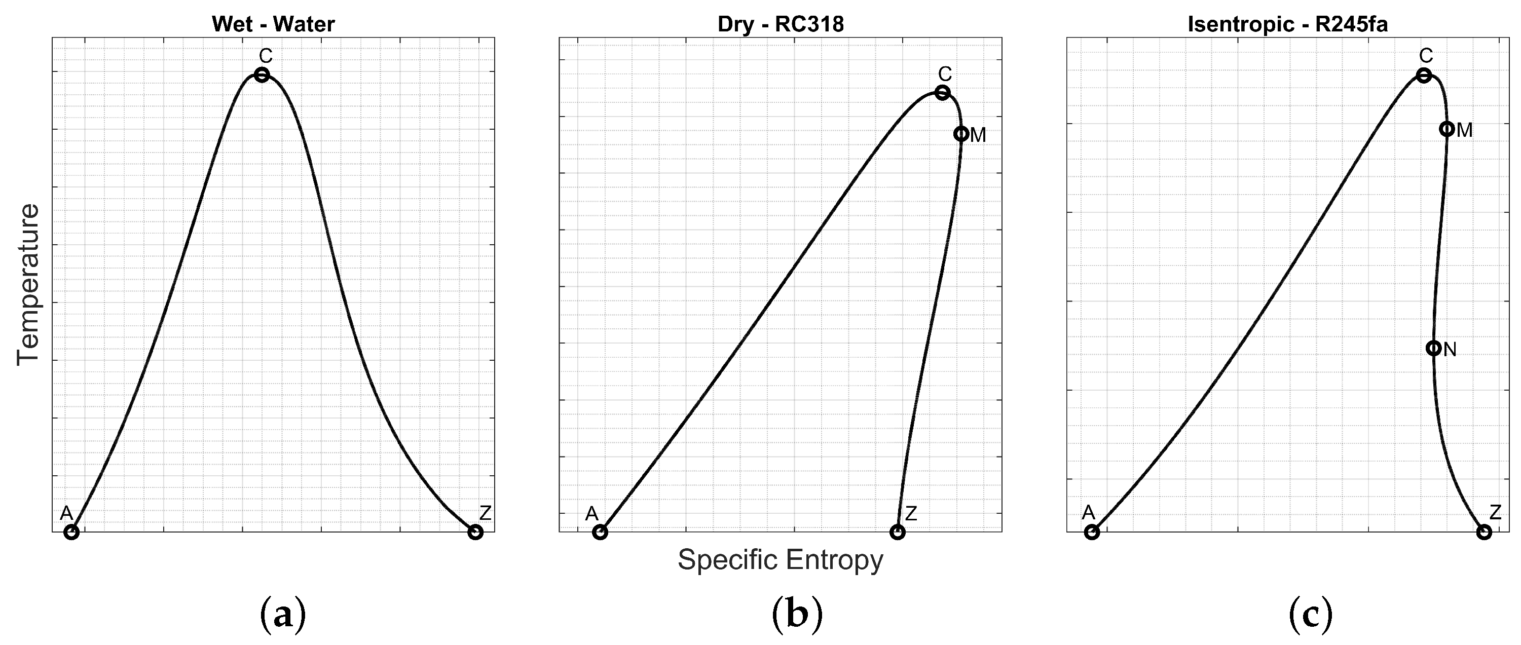
• Wet: a working fluid that has a negatively sloped saturated vapour curve. Examples are water, methane, and refrigerant R32.
• Dry: a working fluid that has a positively sloped saturated vapour curve. Examples are butane, RC318, and Novec649.
• Isentropic: a working fluid which has a near infinite slope; essentially, the saturated vapour line is vertical (or near to). Fluids that are typically categorised as isentropic include pentane and R245fa.

While the three categories as defined above are fairly well established, they have a number of associated limitations when considering thermodynamic power cycles. Consequently, the novel classification proposed by Gyorke et al. [6] is preferable when classifying working fluids for use in thermodynamic power cycles. This system categorises fluids based upon the location of a set of characteristic points as found on their respective Ts-diagrams; the primary characteristic points are depicted for each fluid type on Figure 2. The primary points are as follows:

• A: The first point on the saturation dome.
• C: The critical point.
• Z: The last point on the saturation dome.
• M: The point of maximum entropy between C and Z; only present for dry and isentropic fluids.
• N: The point of minimum entropy between C and Z; only present for isentropic fluids.

These points relate to the location of the minima and maxima along the saturation dome and allow for further expansion of the traditional classification system as shown in Figure 3, where the sequence defining a working fluid is determined by the order in which each point appears as entropy increases.

Working fluid selection is one of the most important aspects of power system design and involves considerations including its impact upon system performance through to safety and environmental concerns.

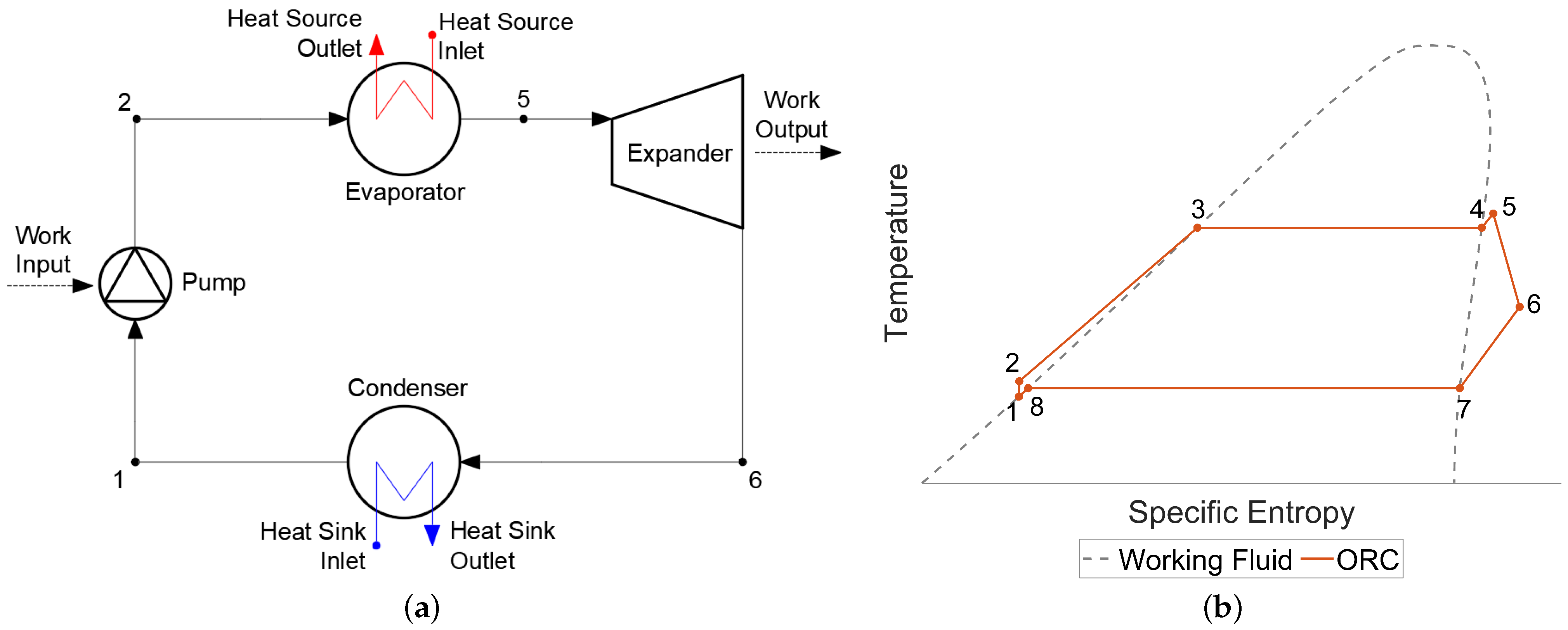
2.1. Organic Rankine Cycle (ORC)

The Organic Rankine Cycle (ORC) is a variation of the well-established Rankine Cycle. The primary difference in the ORC is that rather than employing water as the Rankine Cycle does, it employs an organic working fluid, typically a refrigerant. The use of such working fluids allows for the ORC to handle lower operating temperatures, making it viable for power generation from low-grade heat sources, while also allowing greater versatility in system design and operating ranges [7]. In particular, the ORC is suitable for solar thermal, biomass, combined heat and power, and heat-recovery applications [8]. The basic architecture for the ORC, along with its accompanying temperature-entropy (Ts) diagram, are presented in Figure 4 (note that the pumping process between states 1 and 2 has been exaggerated to increase clarity in Figure 4b), where the processes associated with the cycle are:

• 1–2. Compression of the working fluid by the pump, resulting in a compressed liquid at the evaporator pressure. This process consumes work.
• 2–3. Preheating of the working fluid to a saturated vapour.
• 3–4. Evaporation of the working fluid to a saturated vapour.
• 4–5. Superheating of the working fluid to a superheated vapour.
• 5–6. Expansion of the working fluid in the expander, resulting in a superheated vapour at the condenser pressure and the production of mechanical work.
• 6–7. Desuperheating of the working fluid, resulting in a saturated vapour.
• 7–8. Condensation of the working fluid, resulting in a saturated liquid.
• 8–1. Subcooling of the working fluid, resulting in a compressed liquid.

Note that the cycle described above is premised on the working fluid being of the dry or isentropic type as is typical of the ORC and assumes that heat transfer processes are isobaric (occur at constant pressure), thus neglecting any pressure drops due to losses. As the ORC typically employs turbine-based technology for the expansion process, wet fluids are typically avoided as they may result in the working fluid undergoing a phase change during the expansion cycle; the presence of liquid droplets during this process can adversely impact turbines and cause damage to their blades [9]. Superheating of the working fluid is also typical to avoid both the formation of liquid droplets but also to improve thermal efficiency; however, this is not necessarily true of dry working fluids, which can see an adverse effect on efficiency due to superheating [10]. ORC systems can consequently use a wide variety of prime movers, including positive displacement machines, such as scroll, screw, piston, and roots expanders, which have all been experimentally investigated [11,12,13,14], as well as more novel expansion devices, such as the Tesla turbine [15]. A more comprehensive list of working fluid and expander selections for the ORC can be found in the review by Bao and Zhao [5].

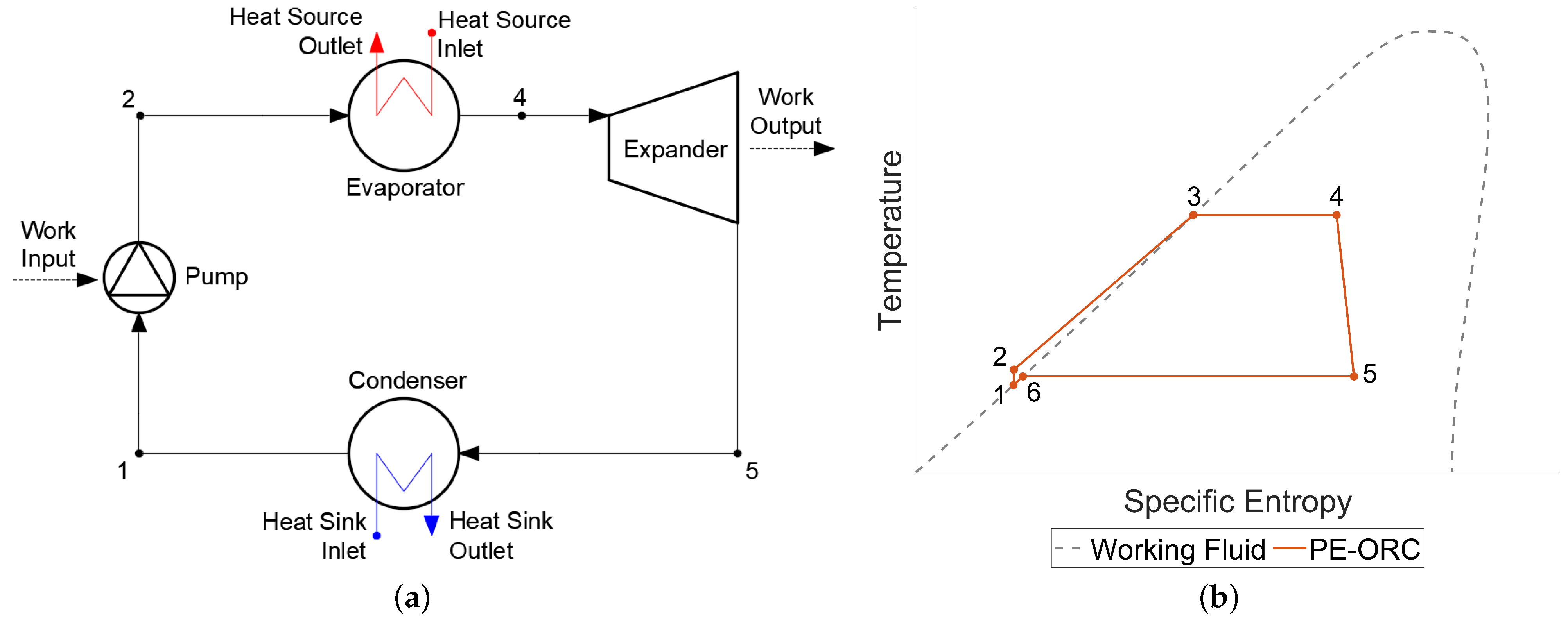
2.2. Partial Evaporation Organic Rankine Cycle (PE-ORC)

The Partial Evaporation Organic Rankine Cycle (PE-ORC) is a variant of the ORC, which, rather than superheating the working fluid, only partially evaporates it. This results in a cycle that begins expansion from a two-phase (liquid–vapour mixture) state. The PE-ORC can achieve higher efficiencies than the ORC due to increased capabilities regarding the manipulation of mass flow rates along with a greater ability to extract heat from the heat source [16,17]. Depending on the operating conditions, the heat transfer associated with the evaporation process can be far closer to the ideal scenario, where the temperature difference between both fluid streams at the inlet and outlet is as close to the pinch-point temperature difference as possible, where the pinch-point represents the point during the heat exchange process where the two fluid streams have a minimum temperature difference. This better matching of heat transfer temperature profiles when compared to the ORC results in more energy being utilised from the heat source and consequent improvements to overall efficiency, particularly for low-temperature applications [18]. The PE-ORC system architecture and accompanying Ts-diagram are presented in Figure 5 and consists of the following processes:

• 1–2. Compression of the working fluid by the pump, resulting in a compressed liquid at the evaporator pressure.
• 2–3. Preheating of the working fluid to a saturated vapour.
• 3–4. Partial evaporation of the working fluid to a two-phase mixture.
• 4–5. Expansion of the working fluid in the expander, resulting in a two-phase mixture
• 6–7. Condensation of the working fluid, resulting in a saturated liquid.
• 7–1. Subcooling of the working fluid, resulting in a compressed liquid.

Like the ORC, the PE-ORC also employs organic working fluids; however, unlike the ORC, wet working fluids need not necessarily be avoided. This is due to the expansion cycle being within the two-phase region, thus necessitating the use of expansion devices that are capable of handling two-phase flow. Consequently, the primary challenge associated with this cycle is the need for such devices, for which positive displacement expanders are typically considered, particularly of the rotary type [16,19,20,21,22].

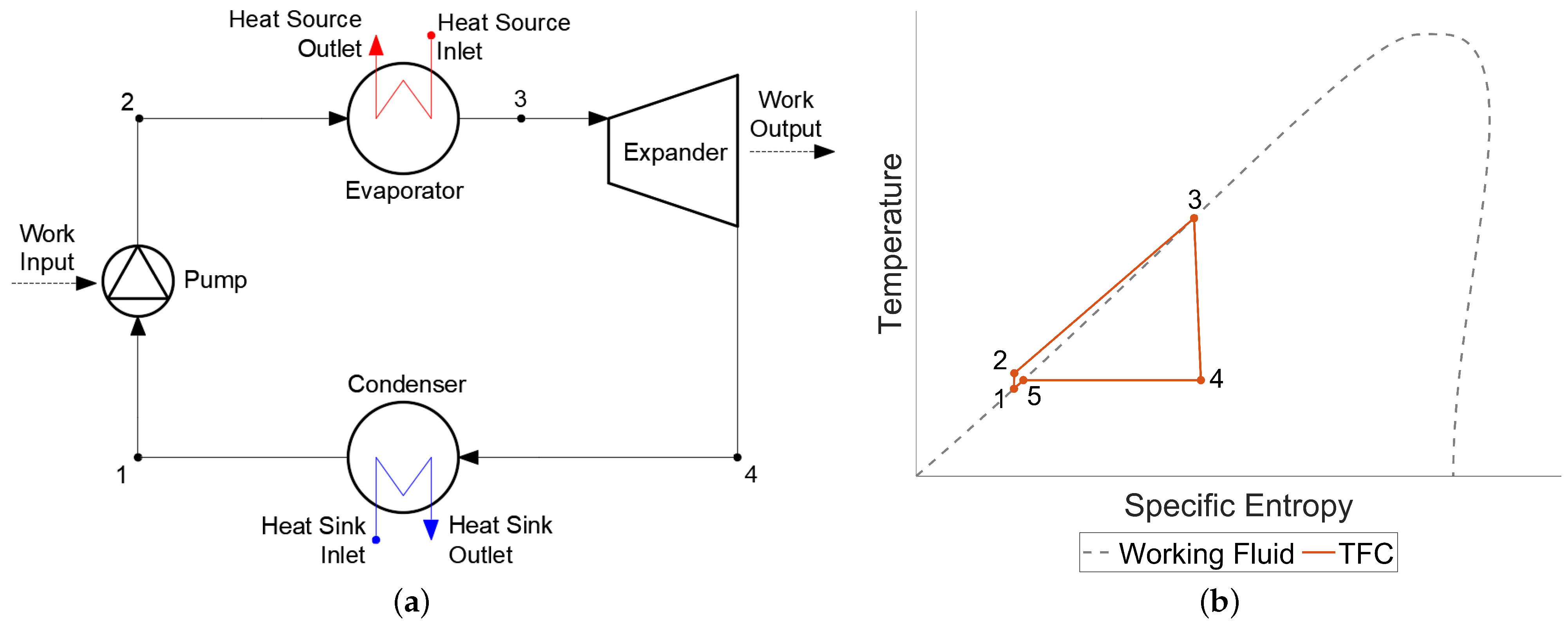
2.3. Trilateral Flash Cycle (TFC)

The Trilateral Flash Cycle (TFC) can be considered as a special case of the PE-ORC, where the evaporation process only goes so far as to boil the working fluid to a saturated liquid state prior to flash-expansion [23]. Similar to the PE-ORC, this results in the expansion process occurring within the two-phase region. The TFC system architecture and accompanying Ts-diagram are presented in Figure 6 and consists of the following processes:

• 1–2. Compression of the working fluid by the pump, resulting in a compressed liquid at the evaporator pressure.
• 2–3. Preheating of the working fluid to a saturated vapour.
• 3–4. Expansion of the working fluid in the expander, resulting in a two-phase mixture
• 4–5. Condensation of the working fluid, resulting in a saturated liquid.
• 5–1. Subcooling of the working fluid, resulting in a compressed liquid.

The TFC is often considered to have the highest theoretical efficiency when considering finite heat sources and was originally conceived for applications with heat sources between 100 and 250 °C [24]. As with the PE-ORC, the efficiencies achievable by the TFC may be higher than the ORC due to the greater possibility of near-ideal heat transfer during the evaporation process [16,25]. Depending on the operating conditions, the TFC may outperform both the ORC and PE-ORC and has the potential to be employed for temperatures below that at which the ORC is viable [25,26,27]. Although the TFC can achieve higher efficiencies than other thermodynamic cycles when considering the improved heat recovery, it does come with the challenge of greater flow rates and the need for expanders capable of handling two-phase flow [25,27]. Experimental work into the TFC typically considers screw expanders as a suitable prime mover [28,29,30].

3. Power Generation System Components

Fundamentally, a power generation system will consist of the four components mentioned in Section 1 and Section 2; a prime mover, pump, evaporator, and condenser. In practice, however, power systems will consist of a great deal more components, such as additional heat exchangers, multiple prime movers and pumps, valves, mixing chambers, and so forth. For the purposes of this paper, this section will introduce some of the most common types of components used within the thermodynamic cycles discussed in Section 2 without consideration of more complex power system designs.

3.1. Heat Exchangers

A heat exchanger is a component that facilitates the transfer of heat between two or more fluid streams; these streams may be liquids, vapours, or liquid–vapour mixtures and may transfer heat either via direct or indirect contact. Within the context of the power generation cycles discussed in Section 2, there are generally at least two heat exchangers that allow for the evaporation and condensation of the working fluid; consequently, these two devices are referred to as evaporators and condensers and indirectly transfer heat without any mixing of fluid streams. While a multitude of different types of heat exchangers exist for various applications, the most commonly used within the thermodynamic cycles discussed in Section 2 are shell-and-tube and plate heat exchangers.

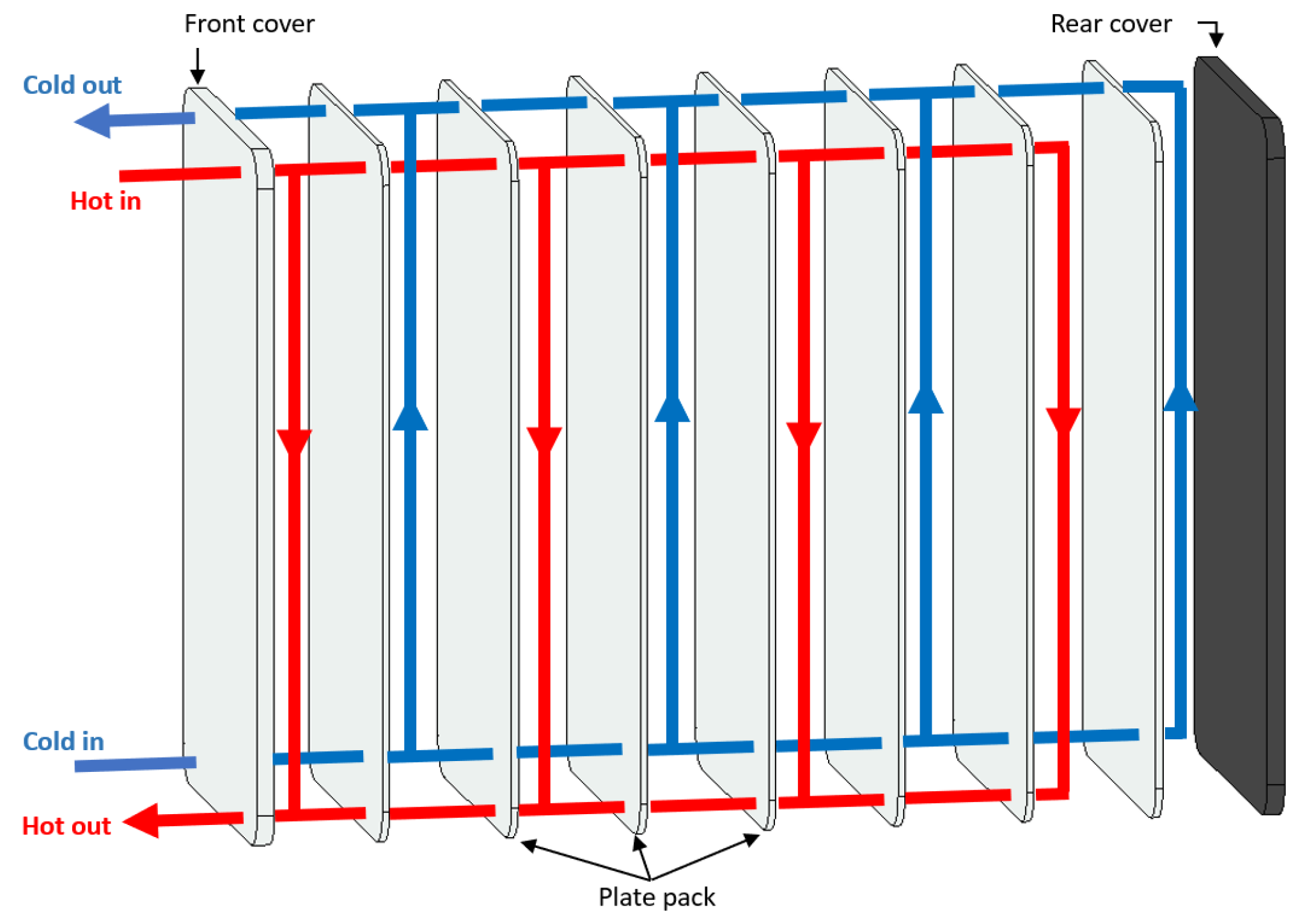
3.1.1. Shell-and-Tube Heat Exchangers

Shell-and-tube heat exchangers consist of an outer shell in which a number of tubes run through. These tubes contain one of the fluid streams while the second fluid is contained outside of these tubes via the outer shell. The shell-side fluid is typically directed by metal plates called baffles which obstruct the flow from the inlet to the outlet, forcing the fluid to continuously change direction and maximise exposure to the outer tube surfaces. This contact with the outer tube surface facilitates the heat transfer between fluid streams. Numerous tubes make a number of runs along the length of the shell, with the contained fluid either accepting or rejecting heat as it flows. The specific application determines which fluid is within the shell or tubes but factors such as fouling and corrosiveness must be considered before deciding whether a fluid should be tube-side. A typical shell-and-tube heat exchanger is presented in Figure 7.

Shell-and-tube heat exchangers are well-established devices used in countless applications; they are relatively simple devices to both manufacture and design and are scaleable and have the advantages of reliability and low cost and are particularly preferred when dealing with liquid fluid streams [31]. The primary disadvantages relate to their large size and fouling within the tube bundles, which requires disassembly and considerable time in order to clean. The sizing of a shell-and-tube heat exchanger can be approached via numerous methods, such as the well-known Bell–Delaware [32] and Kern methods [33] along with the stream analysis method; however, the latter of these is proprietary information and while the method itself has been published, a number of empirical values required in calculations have not been [34]. The primary appeal of shell-and-tube heat exchangers is their reliability, established methods of modelling, cost, and wide availability. While shell-and-tube heat exchangers are used within large-scale power plants, their use within smaller-scale power systems may be disadvantageous as their size and weight may prove to be unsuitable for such applications. Nonetheless, a number of published works have employed them as evaporators and/or condensers within ORC-based systems [35,36].

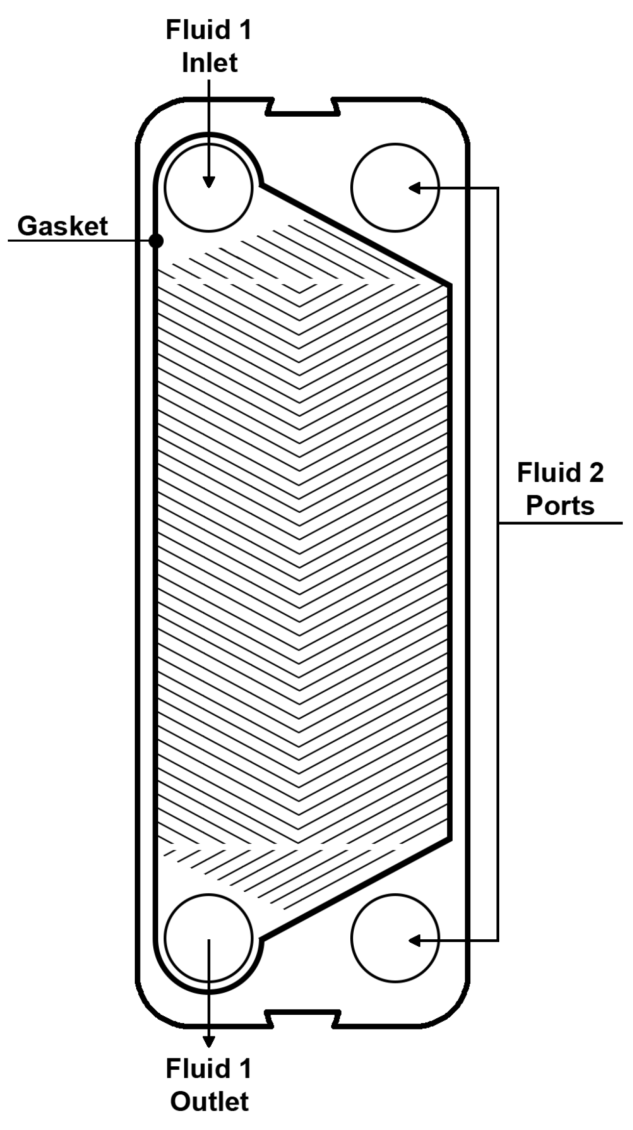
3.1.2. Plate Heat Exchangers

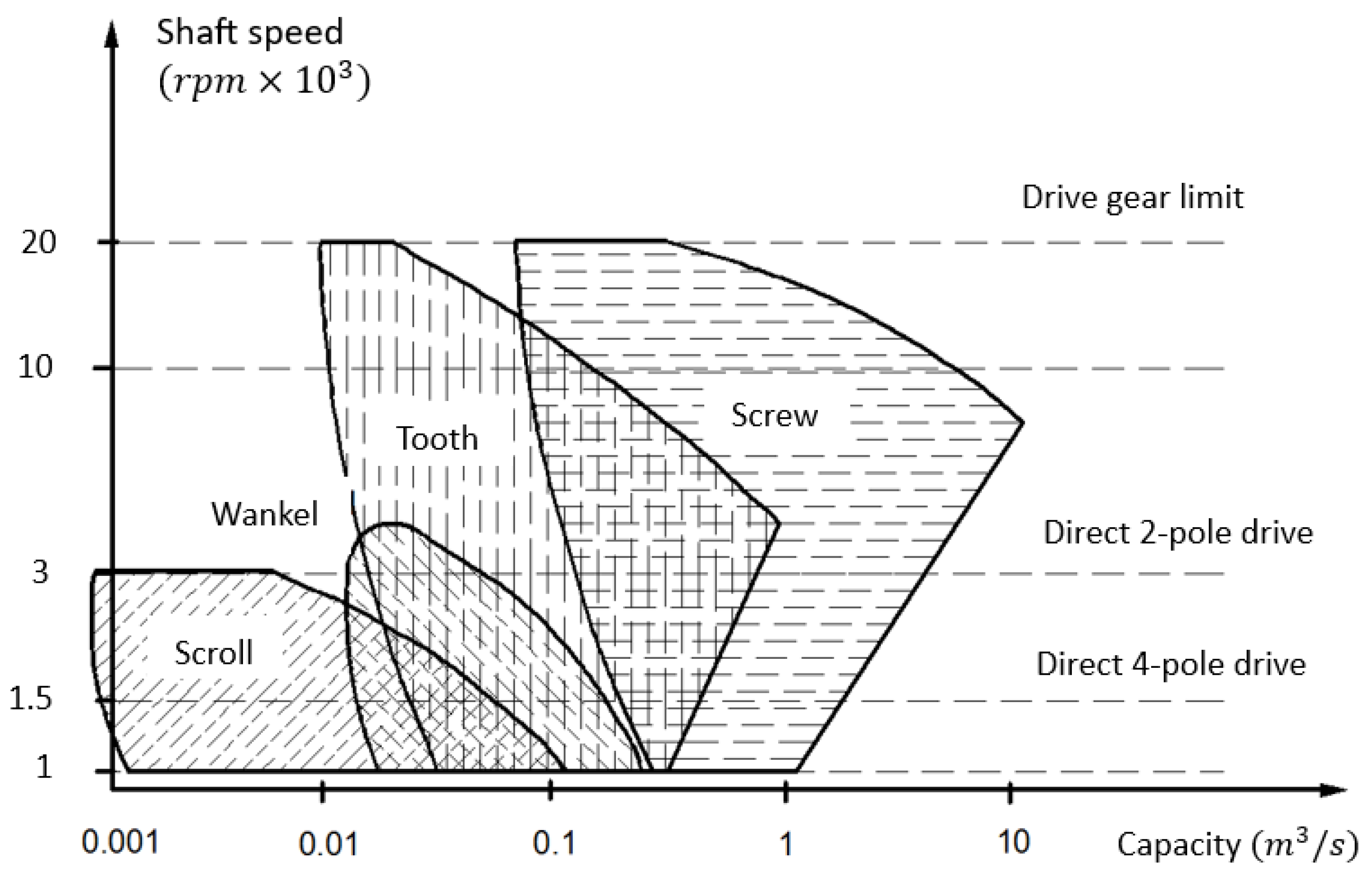
The 1800s saw the rise of milk pasteurisation, which requires that the temperature of the milk is raised to a specific point and maintained there for some period of time in order to eliminate any harmful organisms—a process which necessitates that the equipment used is both highly efficient and is also able to be cleaned regularly with minimal difficulty [37]. To achieve this, plate heat exchangers (PHE) were designed and effectively consist of a number of thin corrugated plates stacked upon each other between each of which an alternating fluid stream flows. These plates are generally held together by a frame and sealed with gaskets or held within a brazed unit depending on the application and any requirements regarding disassembly and cleaning. PHEs tend to be preferred for applications where high efficiencies and small unit sizes are desirable, resulting in their frequent employment within small-scale thermal power systems, such as those based upon the ORC, as evidenced by their use in numerous experimental works [11,14,38,39,40,41,42,43]. An exploded assembly of a PHE is given in Figure 8, while a gasketed plate with a chevron corrugation pattern is given in Figure 9.

As each fluid stream in a PHE flows between two very thin plates (typically, no more than 1 mm in thickness) and is generally made more turbulent by the corrugation pattern of the plates, the heat transfer efficiency tends to be much greater than in shell-and-tube heat exchangers as a result of both the increased contact surface area and turbulence. The increased contact surface area combined with the thin heat transfer media results in much smaller units than would be required by a shell-and-tube heat exchanger of comparable heat duty. While both more efficient and smaller, PHEs are typically more expensive, are produced by a limited number of manufacturers, and are much more complex to model than shell-and-tube heat exchangers. Much information regarding PHEs tends to be proprietary information and manufacturers rarely share any of their modelling techniques. The complexity in modelling PHEs stems from the vast number of design parameters associated with them, including considerations such as the plate geometry, material, and corrugation pattern, the flow arrangement, the gasket material, the number of plates, operating pressures and temperatures, and the fluids employed in each stream. The most well-known and openly available design approaches are the $ϵ$-NTU and LMTD methods [44].

3.2. Prime Movers

Various expander/prime mover designs are suitable for power generation; in this paper, expanders/prime movers are often referred to as expanders. This paper will touch upon different types of expanders, e.g., axial piston, reciprocating piston, rolling piston, revolving vane, scroll, and limaçon expanders, that are suitable for small-scale heat and power-extracting applications; these expanders belong to the positive displacement class of machine. As the name implies, these machines extract work from small portions of the working fluid at a time by allowing fluid to fill their working chambers and expand, increasing volume to transfer the internal energy to the machines’ rotors. This paper then focuses on the limaçon expander technology that has recently reemerged following the advancements made in manufacturing capabilities. Figure 10 below maps the performance of expander designs based on their optimal operation speeds and flow rates; this figure can be used as a preliminary screening guide for the selection of a suitable expander for specific applications. The subsections below will focus on expander designs that are of similar capacity as the scroll expander shown in Figure 10.

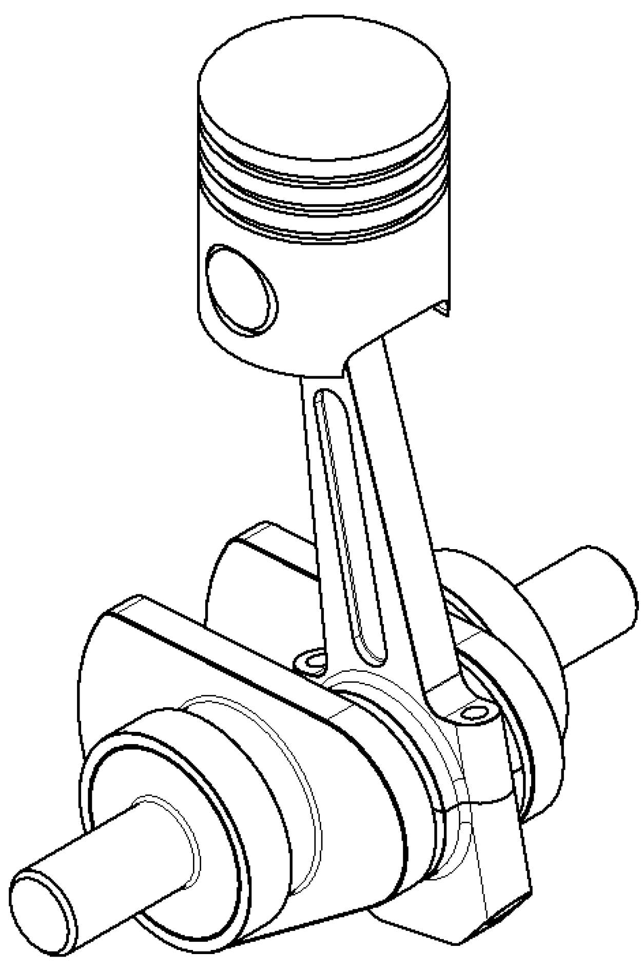
3.3. Reciprocating Piston Expander

The reciprocating piston is the most widely used expander type in many applications, such as internal combustion engines and reciprocating piston compressors. This design employs the conventional crank, rotating link, and slider, reciprocating link mechanism to convert the rotating motion into the reciprocating motion of a piston, in the case of a compressor, or converting the reciprocating motion of a piston to the rotating motion of a shaft, in the case of a combustion engine. As an expander, the input pressure imparts reciprocating motion to the piston, which, through a connecting rod, turns the crankshaft and provides power output at the crank. This type of machine has the direction of motion of the piston and the axial direction of the crank arranged perpendicular to one another; the inlet and outlet valves are often located on top of the piston near the top dead-centre, for the ratio of the maximum to the minimum chambers to be as large as possible. An example of a reciprocating piston expander, without inlet and outlet valves and cylinder block, is shown in Figure 11.

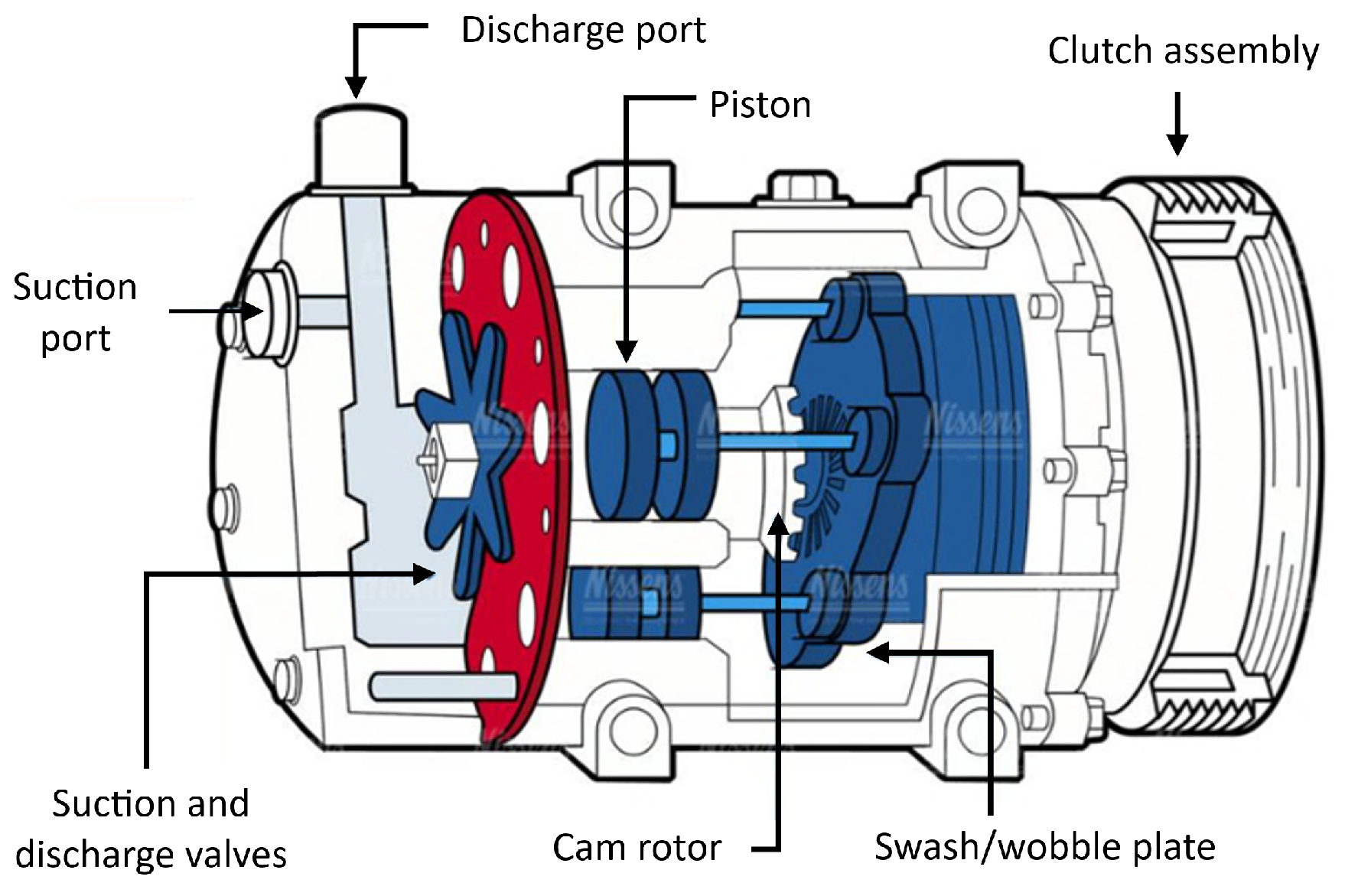
3.4. Axial Piston Expander

An axial piston expander is a different, and often more compact, way to arrange the pistons and machine shaft compared to the reciprocating piston expander above. The pistons are located on axes parallel to the main shaft. By employing a plate tilted on an angle, also known as a swash plate or wobble plate, the rotational motion of the main shaft is translated to the reciprocating motion of the pistons, as shown in [46,47] and in Figure 12; of note is that the motion of the pistons is always aligned with the expander’s main shaft. These machines are mainly employed in automobile applications as air conditioning compressors due to their compactness; another worthy of mention is the Duke engine developed by Duke et al. [48].

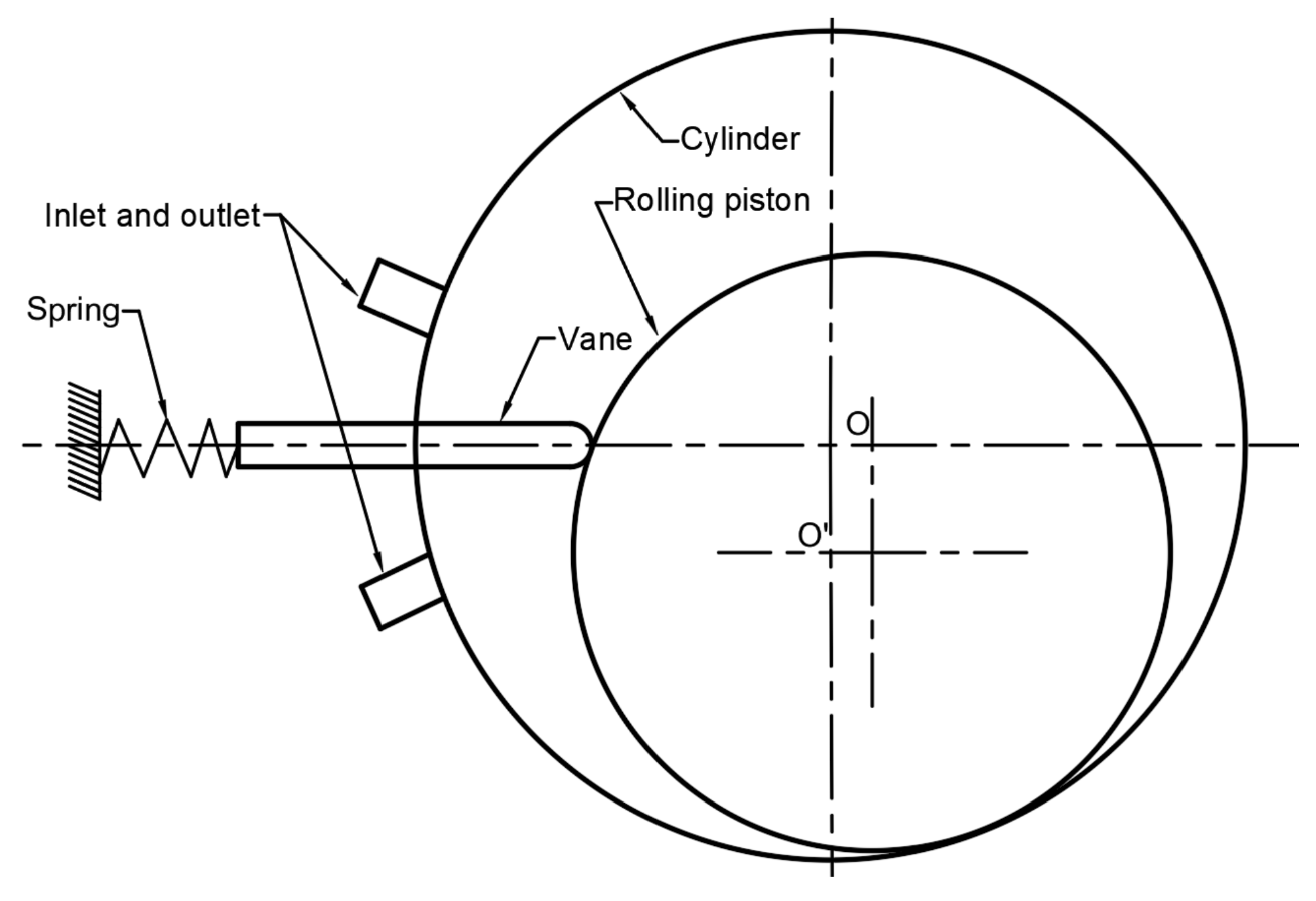
3.5. Rolling Piston Expander

The rolling piston expander, shown in Figure 13, mainly comprises a cylindrical housing and a cylindrical piston that is placed eccentrically to the housing. The piston is allowed to roll on the inside surface of the housing; hence, the name, rolling piston expander. The housing-piston contact separates the two chambers that connect to the expander’s inlet and outlet. A vane extrudes from the housing and touches the piston to form another boundary for the chambers; this vane also separates the inlet from the outlet ports, the amount of extrusion of the vane depending on the relative distance between the piston and housing during the machine operation. This machine can be used as either an expander or a compressor when required.

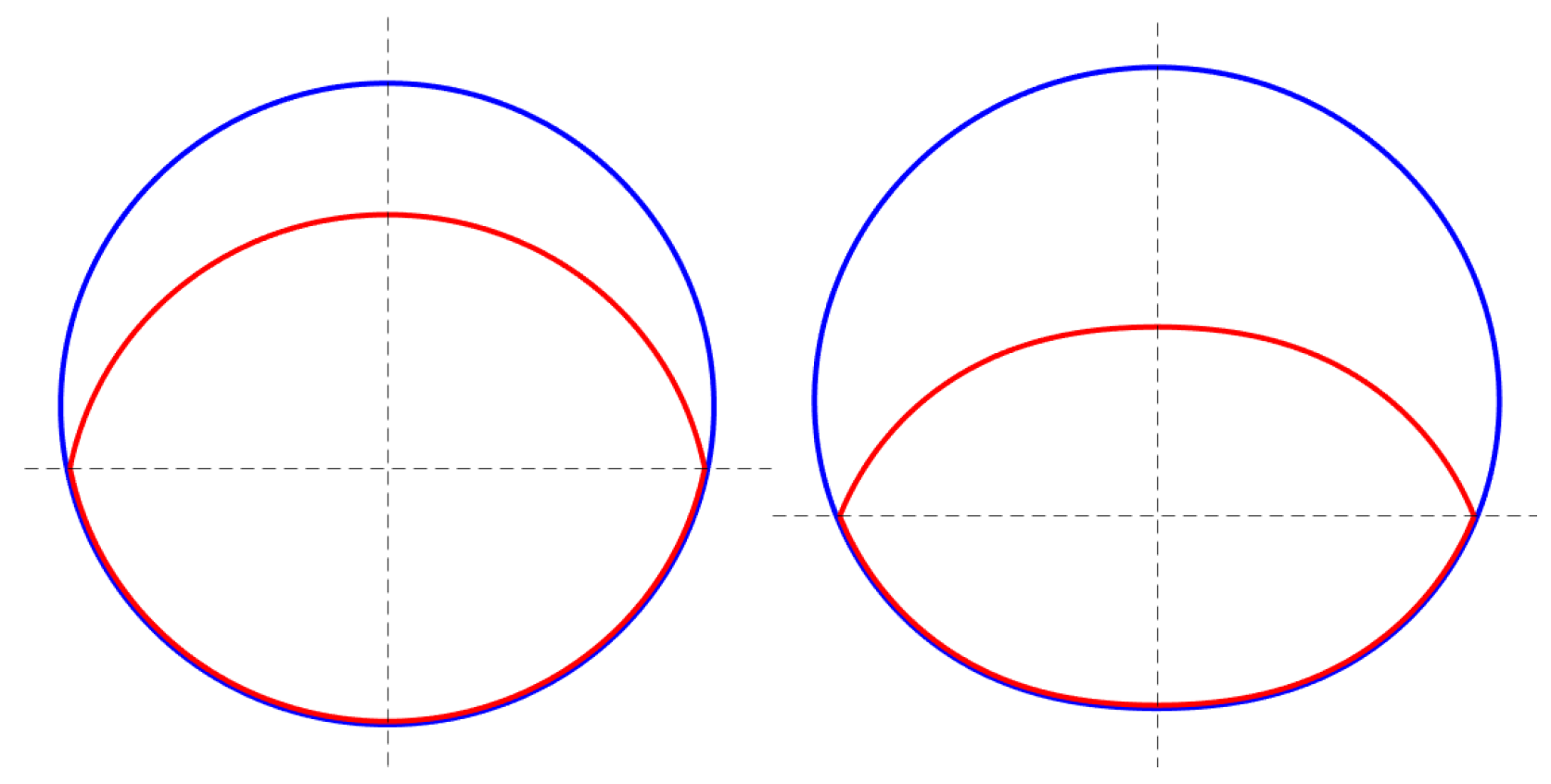
3.6. Rotary Vane Machine

The rotary vane is another type of rotary machine that is widely used in the industry. These machines are often used as oil pumps and/or air motors in automotive and pneumatic applications. The rotary vane machine’s rotor is of cylindrical shape, while the inner cavity of the housing is somewhat ellipsoidal; the machine cavities are formed by the space between the rotor and the inner wall of the housing, as shown in Figure 14. Even though it has a similar cylindrical shape as the rolling piston machine shown above, the rotary vane’s rotor only performs pure rotations about its axis. The vanes protrude from the rotor, touch the inner wall of the housing, and separate the cavities into chambers for fluid-processing purposes. The number of vanes and the positions of the inlet and outlet depend on particular designs and the type of fluid to be processed.

3.7. Scroll Expander

Scroll expanders belong to the family of orbital machines. These machines have two involutes, as shown in [49], and in Figure 15 below, one involute is the central symmetry of the other. As the machine operates, the volume trapped between the two involutes changes, which can be taken advantage of for processing working fluids, as either an expander or a compressor; the type of machine will depend on the locations of the ports and the direction of rotation. One major operational constraint of this expander is the temperature of the working fluid at the expander inlet. Research has shown that high temperature leads to thermal stress developing in the scrolls and results in leakage losses and reduced seal performance.

3.8. Limaçon Machine

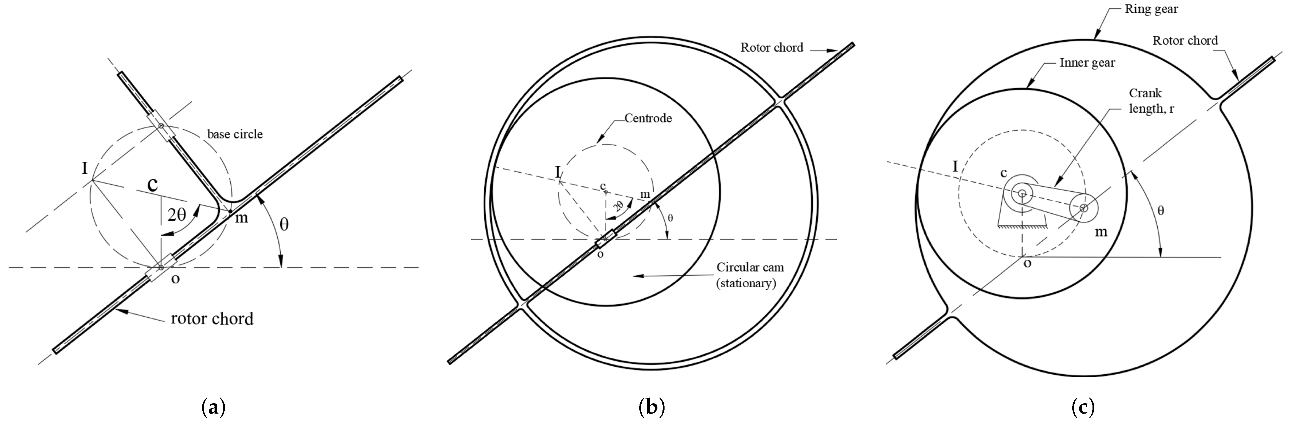
This section details the design of the limaçon expander; the mathematical models that define the machine geometries and differentiate various machine embodiments from the original limaçon of Pascal curve will be presented. An example of a limaçon machine is shown in Figure 16. This machine comprises a stationary housing and a rotor of lenticular shape, that rotates, following a limaçon curve (or snail curve, because half of the curve above the x-axis looks like a snail shell with part of the whorl visible), as shown in Figure 17, inside. The spaces between the housing’s inner wall and the rotor’s profile form the machine chambers. Of particular note is that two chambers exist at the same time; one is above and one is below the moving line $p_1{p}_2$ (more on this is provided a bit later in the paper). The chambers’ volumes vary with the angular displacement of the rotor, making this machine suitable for fluid processing, e.g., compressors, expanders, or pumps [50,51,52]. The profiles of the machine’s housing and rotor can be of either limaçon or circular curves; the motion of the rotor inside the housing has to strictly follow the limaçon motion for the machine to work properly.

The limaçon machine design can be traced back to the 19th century and has been refined and redesigned by researchers as shown in their published works and pate- nts [50,51,54,55,56,57]. The utilised limaçon curve takes either of the polar forms

$$r=a+bcos\left(\theta \right)$$

(2)

$$r=a+bsin\left(\theta \right)$$

(3)

where the $cosin$ curve, Equation (2), takes the x-axis as its mirror line, while the $sin$ curve, Equation (3), takes the y-axis as its mirror line.

To apply the curves to the limaçon machine, some definitions of the machine geometries need to be included in either of the equations above. As shown in Figure 16, the two-lobe-shaped machine rotor is symmetrical about a line connecting the two apices $p_1{p}_2$, called the rotor chord. Point m is the centre point of the chord, and the half-chord length, L, is defined as the distance between m and $p_1$ (or $p_2$).

For the limaçon shape and motion to be realised, we need to define a pole, o, attached to which are the fixed coordinates $XY$. The centre of a base circle of radius r lies on the positive side of the y-axis and at a distance r from the pole. The limaçon motion is formed as the chord, $p_1{p}_2$, rotates and slides about the pole, o, while the midpoint of the chord, m, stays kinematically attached to the base circle. The distance between o and m changes as the chord performs its motion; this is the sliding distance, s, and can be expressed as a function of r and $\theta$, measured between the positive (+ve) x-axis and the rotor chord, as:

$$s=2rsin\left(\theta \right)$$

(4)

It is necessary to define a moving frame, $X_r{Y}_r$ attached to point m of the rotor and which rotates with it, as shown in Figure 16. Now, the point m is the origin of frame $X_r{Y}_r$ and the point o is the origin of the frame $XY$. The sliding distance, s, is, in fact, the distance between these two origins. As the rotor rotates, the traces of point $p_1$ (or $p_2$) form the limacon curve, which is also the shape of the machine housing. This can be represented as the radial distance of the rotor housing, $R_h=s+L$,

$$R_h=2rsin\left(\theta \right)+L$$

(5)

This polar form of the housing can be transformed to the Cartesian coordinates as:

$$\left\{\begin{array}{c}{x}_h=rsin\left(2\theta \right)+Lcos\left(\theta \right)\hfill \\ y_h=r[1-cos\left(2\theta \right)]+Lsin\left(\theta \right)\hfill \end{array}\right.$$

(6)

Of note is that the limaçon can have loops, dimples, and kinks, as shown in Figure 17. To be used as a machine, this curve has to be free from dimples and kinks [58], which means the ratio between the base circle radius, r, and the half-chord length, L, has to be less than 0.25 $(b=r/L<0.25)$. Figure 18 depicts two pairs of housing and rotor combinations, one with $b=0.1$ and the other with $b=0.2$; note that the half-chord length, L, is kept constant in these cases. Figure 18 also shows that as the value of b increases, the limaçon curve will start to squeeze on one end, the bottom end as in the figure; the dimple will start to form as b is further increased beyond the limit of 0.25.

In the context of a positive displacement machine, the housing will be provided with ports for the fluid to flow into the machine chamber (inlet) and discharge from the machine (outlet), as shown in Figure 16 above.

3.8.1. Embodiments

Currently, there are three housing-rotor combinations whereby the housing and rotors are manufactured using either the limaçon or circular curves; of note is that the rotor motion inside the housing always follows the limaçon motion. These embodiments are:

• Limaçon-to-limaçon (L2L) machine: the housing and rotor are both manufactured to the limaçon curves,
• Circolimaçon (CL) machine: the housing and rotor are manufactured to the circular curves,
• Limaçon-to-circular (L2C) machine: the housing is of the limaçon curve while the rotor is manufactured to the circular curve.

The differences in these arrangements are shown in Figure 19 below:

Given the same half-chord length, L, and ratio b, the L2L machine has the largest chamber volume ratio. The ratio between the largest and smallest chamber volumes, and the gap between the rotor apices and the housing is kept constant, due to the nature of this machine, during the machine operation. The CL machine, on the other hand, is simpler to manufacture due to the circular shapes of the housing and rotor. However, the rotor apex and housing distance of the CL machine vary significantly during the operation, which makes apex sealing more challenging. The L2C machine has the advantage of both the above embodiments. This machine slightly sacrifices the volume ratio while maintaining the sealing effectiveness of the L2L machine.

Due to the particular shapes of the rotor and housing that form two working chambers, one above and one below the rotor chord, $p_1{p}_2$, together with the unique limaçon motion, this type of machine can process the fluids twice per rotor revolution. This is equivalent to two power strokes per rotor cycle.

The mathematical models of the L2L, CL, and L2C are presented below. Of note is that this paper only presents the housing and rotor profiles and the volumetric relationship of the machine based on the profile. More details on other aspects of these machines can be found in the works by Sultan et al. [51,57,59] for L2L, Cl, and L2C machines, respectively.

• Limaçon-to-limaçon (L2L) machine

First, the limaçon-to-limaçon (L2L) machine, shown Figure 19 left, housing and rotor are defined in the polar coordinates, respectively, as:

$$\left\{\begin{array}{c}{R}_h=L+2rsin\left(\theta \right)\hfill \\ R_r=2r_{r}sin\left(\varphi \right)+(L-C)\hfill \end{array}\right.$$

(7)

where C is a small clearance that is introduced to the rotor shape definition, which shortens the rotor chord by a small value, to prevent the interference between the machine housing and rotor; $r_r$ is the radius of the rotor base circle and is calculated based on L, C, and the same value of b as the housing. In a similar manner to the way angle $\theta$ is utilised to form the housing, the angle $\varphi$ is utilised to form the rotor shape. From these, Cartesian representations of the housing profile can be expressed as in Equation (6) and rotor profiles can be expressed as below:

$$\left\{\begin{array}{c}{x}_{rl}=x_{ru}=r_{r}sin\left(2\varphi \right)+(L-C)cos\left(\varphi \right)\hfill \\ y_{rl}=y_{ru}=r_r[1-cos\left(2\varphi \right)]+(L-C)sin\left(\varphi \right)\hfill \end{array}\right.$$

(8)

where $(x_{rl},y_{rl})$ and $(x_{ru},y_{ru})$ are the profiles of the lower part and upper part of the rotor, respectively.

To calculate the chamber volumes available for fluid processing, first, the areas of the housing above and below the chord and the area of half the rotor, $A_a,A_b,A_r$, respectively, need to be calculated.

$$\begin{array}{c}{A}_{a,b}=\pi \left(r^2+{\displaystyle \frac{1}{2}}{L}^2\right)\pm 4rLcos\left(\theta \right)\\ A_r=\pi \left(r_r^2+{\displaystyle \frac{1}{2}}{L}^2\right)-\pi C\left(L-{\displaystyle \frac{1}{2}}C\right)-4r_r(L-C)\end{array}$$

(9)

where the ± signs signify the calculations for above and below the chord, respectively.

The differences between these areas, $A_a-A_r$ and $A_b-A_r$, are the machine chambers’s cross-sectional areas. The volumes of these chambers, $V_a=H(A_a-A_r)$ and $V_b=H(A_b-A_r)$, can be calculated based on these cross-sectional areas and the machine depth, H, measured perpendicular to the page as

$$V_{a,b}=H\left[\pi \left(r^2-r_r^2\right)+\pi C\left(L-{\displaystyle \frac{1}{2}}C\right)+4r_r\left(L-C\right)\pm 4rLcos\left(\theta \right)\right]$$

(10)

Based on the points above, other aspects of the L2L machine can be calculated.

• Circolimaçon (CL) machine

As for the CL machine, both the housing and rotor are of circular curves; as such, the distance between the rotor apex and the housing varies as the rotor rotates. $R_h$ is the housing radius and d is defined as the apex-housing distance, or apex gap, as shown in Figure 19 middle. The housing centre, $O_h$, is at a distance Z above the pole, o, on the positive y-axis. The relationship between these geometric values is expressed as

$$R_h^2=Z^2+{(L-C+s+d)}^2-2Z(L-C+s+d)cos\left(\psi \right)$$

(11)

where $\psi =\pi /2-\theta$. Based on Equation (11) and some design conditions of d as detailed by Sultan [57], and $Z=2r$, the expression for the apex gap, d, can be derived as

$$d=-L+C+L\sqrt{1+b^{2}sin{\left(\theta \right)}^2}$$

(12)

The CL rotor arc can be expressed as

$$R_r=\sqrt{4k^2{r}^2+{(L-C)}^2}$$

(13)

where $k=a\left(1-{\displaystyle \frac{C}{L}}\right)$, where $a\ge 1$; a can be selected by the designer or calculated to suit the machine’s desirable performance criteria [57]. The centre of the rotor arc, $O_r$, lies on a line that connects the chord centre point, m, and the housing centre, $O_h$; and $O_r$ and m are opposite one another about $O_h$.

The cross-sectional areas of the housing above and below the rotor chord, respectively, can be calculated as

$$A_{a,b}=L^2\left[\left(1+4b^2\right)\left({\displaystyle \frac{\pi }{2}}\pm {\lambda }_h\right)\pm 2bcos\left(\theta \right)\sqrt{1+4b^{2}sin{\left(\theta \right)}^2}\right]$$

(14)

where ± signs signify the calculations for above and below the chord, respectively, and ${\lambda }_h=ta{n}^{-}1\left({\displaystyle \frac{2rcos\left(\theta \right)}{L-C+d}}\right)$. The rotor half-cross-sectional area is

$$A_r=R_r^2{\beta }_r^2-2kr(L-C)$$

(15)

where ${\beta }_r={\displaystyle \frac{\pi }{2}}-{\lambda }_r$ and ${\lambda }_r=ta{n}^{-}1\left({\displaystyle \frac{2kb}{1-C/L}}\right)$. Hence, the chamber volume above and below the chord can be calculated based on the machine depth, H, and the rotor and housing areas as

$$\left\{\begin{array}{c}{V}_a=H(A_a-A_r)\hfill \\ V_b=H(A_b-A_r)\hfill \end{array}\right.$$

(16)

From the points above, other aspects of the CL machines can be calculated.

• Limaçon-to-circular (L2C) machine

The L2C machine, shown in Figure 19 right, housing has a similar limaçon profile to that of the L2L machine presented above, half of the cross-sectional area of the lenticular rotor; however, it takes a circular flank shape, the radius of which can be expressed as,

$$R_r=\sqrt{4k^2{r}^2+{(L-C)}^2}$$

(17)

the arrangement of the rotor centre, $O_r$, is similar to that of the CL machine. The coefficient k in Equation (17) can be calculated based on the condition $k>{\displaystyle \frac{1-C/L}{\sqrt{1-4b^2}}}$. The housing and rotor areas, respectively, can be calculated as,

$$\begin{array}{c}{A}_h=L^2\left[\left(b^2+{\displaystyle \frac{1}{2}}\right)\pi +4bcos\left(\theta \right)\right]\\ A_r=\left[{\left(L-C\right)}^2+{\left(2rk\right)}^2\right]\phi -(L-C)2rk\end{array}$$

(18)

The difference between the housing area and the rotor area is called $A_{net}=A_h-A_r$; therefore, the machine volume chamber can be calculated as $V_{net}=A_{net}H$, where H is the machine depth measured perpendicular to the page. From here, the machine’s aspects can be calculated with similar approaches as the L2L and CL machines above.

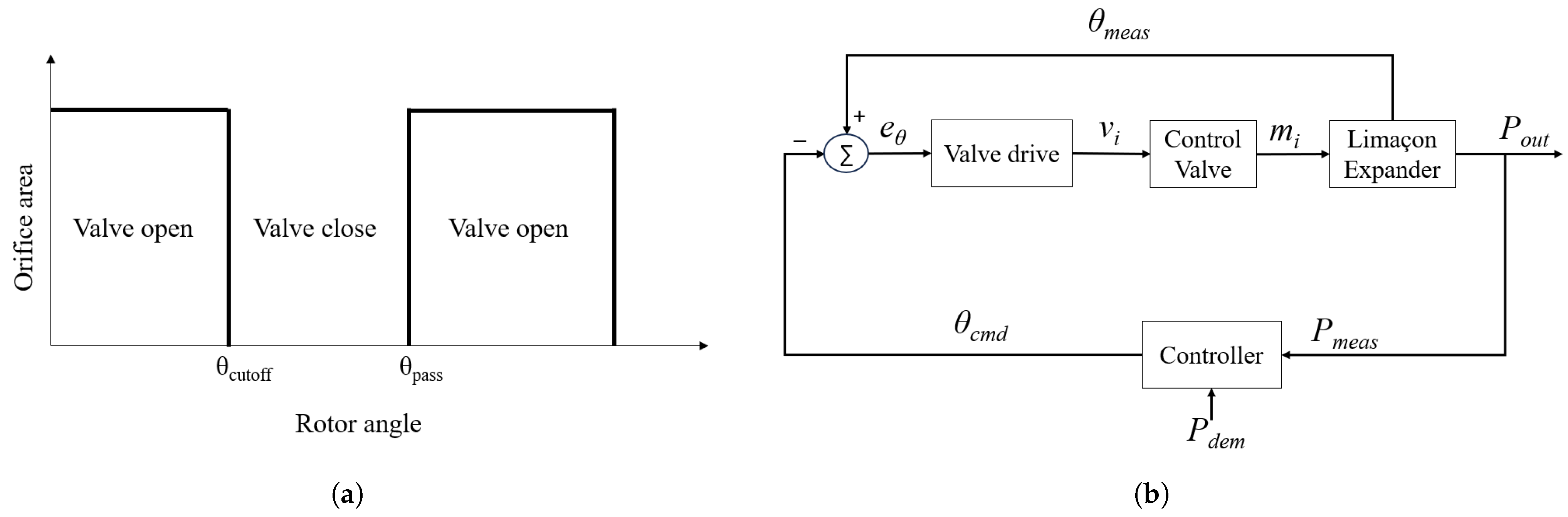
3.8.2. Inlet and Outlet Port Positions and Areas

The inlet and outlet port positions and areas for the limaçon machine have been developed by Sultan et al. [60,61], which can be applied for L2L, CL, and L2C machines. The approach defines the leading and trailing vectors for the leading and trailing edges of the ports; this concept treats the inlet and outlet ports without discrimination.

$$\left\{\begin{array}{c}{\mathbf{R}}_l=L\left(2bsin\left({\theta }_l\right)+1\right){\widehat{\mathbf{R}}}_l\hfill \\ {\mathbf{R}}_t=L\left(2bsin\left({\theta }_t\right)+1\right){\widehat{\mathbf{R}}}_t\hfill \end{array}\right.$$

(19)

where ${\theta }_l$ and ${\theta }_t$ are the leading and trailing edges’ angular positions, respectively, and ${\widehat{\mathbf{R}}}_l$ and ${\widehat{\mathbf{R}}}_t$ are the unit vectors. Based on these, the port angular width, W, and the port area, $A_f$, can be calculated as

$$\begin{array}{c}W=|{\widehat{\mathbf{R}}}_l-{\widehat{\mathbf{R}}}_t|\\ A_f=L_{P}W-W^2\left(1-{\displaystyle \frac{\pi }{4}}\right)\end{array}$$

(20)

where $L_p$ is the port length measured perpendicular to the page and $L_p<H$. This particular area, $A_f$, is based on the assumption that the ports take the stadium shape, a rectangle with two half-circles at the two ends, as shown in Figure 20. The angular positions of the port leading edges are defined based on the thermodynamic performance and the working conditions of the machine.

3.8.3. Limaçon Drive

This section will investigate different mechanisms that can produce the limaçon motion and at the same time can achieve the desirable two power strokes per cycle that can be used to drive the limaçon machines. First, the limaçon motion needs to be summarised and based on that, the number of suitable linkages can be narrowed down.

• the midpoint, m, if the rotor chord, $p_1{p}_2$, remains attached to the circumference of the base circle and rotates about the centre of that circle at twice the angular speed of the chord itself about m.
• the chord is permanently attached to the pole, o, of the machine, the origin of the fixed $XY$ frame, about which the chord can rotate and slide.
• the instantaneous centre of velocity of the rotor falls on the base circle and diametrically opposite the rotor midpoint, m. The base circle can be considered as the centrode of the linkage.

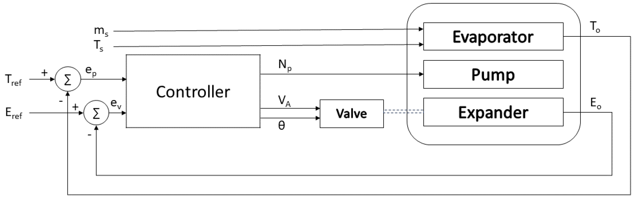
A few designs can satisfy the requirements above, such as the cam-assisted drive, shown in Figure 21b [62], where the rotor is equipped with a circular rolling surface between the rotor and the stationary cam. At the same time, there is a sliding surface between the rotor chord and a slider located at the pole, o. The epicycloidal gear drive is another potential option for this application. Shown in Figure 21c is a simplified schematic of a generic epicycloidal gear presented by Moore [63]. These two designs, based on the implementation, have minimum sliding surfaces; therefore, the lubrication method can be kept fairly simple.

A double-slider design utilises two perpendicular sliders , shown in Figure 21a, and its variations have been proposed and investigated by different inventors [55,64,65]. This design produces limaçon motion since point m of the chord always falls on the base circle; one of the pivots is at the pole, o. The distance between the two pivot points is equal to the diameter of the base circle. This mechanism employs sliding motion on flat surfaces and is expected to have mechanical losses; this can be reduced with proper bearing design and lubric- ation methods.

4. Control System

Power generation systems require robust control strategies to account for variations in the form of changes in load demand and disturbances to operating conditions. If the required power output fluctuates, the system should adjust its operation to account for this. Similarly, if internal or external disturbances occur, the system needs to be able to account for these to ensure consistent, safe, and efficient operation. This is typically achieved through variation of one or more of the operating parameters, such as the mass flow rate, degree of superheating, evaporation pressure, etc. Manipulation of such parameters can typically be achieved by varying the power input to the pump or by employing valves. Strategies vary based on the thermodynamic system employed, depending on the system design and thermodynamic cycle employed. The following section will first discuss control within the context of thermodynamic cycles and follow this with a discussion of control specific to limaçon expanders.

4.1. Cycle Control

An efficient, fast, and dynamic control system is necessary to maintain the intended performance of a power cycle and handle any internal and external disturbances. For this, a process control loop incorporating a fast-acting control valve can be implemented. Control loops are the fundamental units of a control system comprising controllers, sensors, and final control elements (FCEs) functioning in tandem to maintain a process variable (PV) as close as possible to the desired set point (SP). A PV can be any system parameter, including the connected load, pressure, temperature, flow rate, and so on. Small-scale power generating units typically employ heat sources that are intermittent in nature whose temperature ($T_s$) and mass flow rate ($m_s$) vary over time. An excessive temperature might degrade or decompose the working fluid and damage system components, whereas a substandard temperature might result in a two-phase working fluid inside the limaçon expander, reducing its efficiency. Therefore, it is necessary to control and stabilise the evaporator outlet temperature ($T_o$) within a predefined range ($T_{ref}$) depending on the components’ ratings and load demand. This can be done by controlling the pump speed ($N_p$). Furthermore, the expander output energy ($E_o$) depends on the inlet mass flow rate and pressure. An inlet control valve can be utilised to control the energy output to a predefined set point ($E_{ref}$) by regulating the amount of fluid entering the expander chamber. This can be accomplished by setting two parameters: (1) the effective valve area ($V_A$) and (2) the expander rotor position ($\theta$), where the valve needs to operate. A schematic of a control loop for a typical power cycle such as ORC is shown in Figure 22.

However, regulating the supply pressure by throttling would result in a loss of energy, reducing the overall process efficiency. Thus, it is preferable to keep the pump speed constant and utilise the expander inlet control valve for process control. The most commonly employed control strategies (within the context of the ORC) include the sliding pressure and constant pressure strategies along with a combination of the two [11,66].

4.2. Expander Control

A limaçon expander, as shown in Figure 16, converts the stored potential energy of the compressed fluid into mechanical energy by enabling the fluid to expand within the expander chamber, resulting in a rotation of the rotor. To ensure optimum performance, it is necessary to regulate the amount of fluid entering the expander chamber. This type of machine is sometimes equipped with a cam-operated valve. However, this type of valve is mechanically coupled with the motion of the rotor and thus has a fixed response and can not be controlled to function in any other way. Since the fluid entering the chamber is not regulated, the compressed fluid fills the entire control volume and is unable to expand. Consequently, a significant portion of the expensive fluid is expelled through the discharge port before it has the opportunity to expand adiabatically within the chamber. Thus, much of the potential energy is wasted in this process. This energy wastage can be avoided by utilising a fast response and variable timing inlet controlled valve in place of a fixed response inlet valve. This is illustrated in Figure 23, where a controlled valve with flexible operation can regulate the fluid flow and allow adiabatic expansion to improve expander efficiency.

The addition of a control valve with a proper control mechanism is able to control the output energy by adjusting the fluid flow. This enables the limaçon expander and the associated power cycle to cope with external load variation, a common phenomenon in real-world applications. Additionally, the adjustable characteristics of the inlet valve allow for an initial high fluid flow to provide the extra torque needed to push-start the rotor and subsequent deregulation of the flow rate to meet load demand only once the rated speed is reached. An ideal control valve should be able to direct the flow of working fluid without any external leakage and withstand operational temperature, pressure, corrosion, erosion, and other factors that can affect actuation.

A controller implements the desired control strategy to actuate the control valve. The controller’s objective is to actuate the valve at certain rotor positions, as shown in Figure 24a, to control the mass flow and achieve the desired output demand and performance characteristics. At the start of the cycle, the valve remains open to allow unrestricted flow till the rotor position ${\theta }_{cutoff}$, where the valve closes to restrict the flow before opening at ${\theta }_{pass}$ to start a new cycle.

Figure 24b shows a generalised block diagram of a limaçon expander control system, where the controller determines the valve actuation angles ${\theta }_{cmd}=\left[{\theta }_{cutoff}{\theta }_{pass}\right]$ to achieve a given output power demand, $P_{dem}$. The valve drive circuit then sends the actuation signal, $v_i$, by comparing ${\theta }_{cmd}$ with the current rotor position, ${\theta }_{meas}$, ensuring a total mass flow of $m_i$. This controller block is a simplified version and can include other measurement and controller blocks depending on the power cycle components and control goals.

Controller Designs

In recent years, several control schemes, including linear, adaptive, and robust control techniques have been utilised to control and stabilise dynamic and fast valve actuation systems [67,68,69,70,71,72]. However, linear control schemes such as proportional-integral-derivative (PID) [73,74] would be difficult to implement in valved-expander systems having nonlinearities, uncertainties, and interference. Moreover, PID controllers’ gain parameters may require frequent tuning, making them inefficient for nonlinear dynamic systems, such as the valved limaçon expander. This issue can be addressed by employing feedback linearisation [75,76,77] in conjunction with a PID controller. However, the linearisation of a nonlinear system could result in system instability from uncertainties in system modelling. In contrast, a model predictive controller (MPC) can account for system uncertainties and nonlinearities provided an accurate system model is available [78,79]. Comparatively, sliding mode controllers (SMC) [68,80,81,82,83], with their variable structural characteristics, could offer improved accuracy and robustness if the associated chattering effect [84] is negated. However, model-dependent controllers like MPC and SMC could show sub-optimal performance if the system model is inaccurate or complex.

The controllers above have previously been utilised to control complex electro-hydraulic systems like the valved-expander system. However, stabilisation of a complex nonlinear system with only one controller is difficult. A hybrid controller implementation would be preferable. For instance, the incorporation of fuzzy logic has been demonstrated to improve the performance of popular controllers, such as PIDs and SMCs [85,86,87]. Similar but simpler predictive controller designs using artificial neural networks (ANNs) [88,89] could be an effective solution for controlling limaçon expanders as they can efficiently operate without a comprehensive system model. A trained ANN model can capture underlying system complexities and uncertainties and effectively predict complex system behaviour by observing past system responses. However, the training process is complex, accruing costs in terms of time and computational resources.

5. Conclusions

Limaçon-based expanders are versatile rotary positive displacement machines which can be employed within various applications, with particular viability within power generation and heat-recovery systems. Small- and micro-scale power systems can benefit from this technology, which can be employed as an efficient and reliable prime mover within thermodynamic cycle-based power systems. Cycles such as the Organic Rankine Cycle (ORC), Partial Evaporation Organic Rankine Cycle (PE-ORC), and Trilateral Flash Cycle (TFC) can implement limaçon expanders due to their ability to handle various operating conditions along with two-phase flow, which is a major challenge when considering the latter two of these cycles. Due to advances in manufacturing capabilities, limaçon expanders are able to be manufactured with relative ease and as several embodiments exist, production costs can be varied depending on operational and budgetary needs. Limaçon expanders allow for the further development of renewable-based energy systems and can be employed within next-generation energy systems involving hydrogen generation. The employment of internal seals and control valves can further improve the viability and performance of limaçon expanders and broaden the range of viable applications. Limaçon technology represents an innovative pathway into the future of fluid-processing technologies and provides additional means towards developing the next generation of power systems.

References

1. Moran, M.; Shapiro, H.; Boettner, D.; Bailey, M. Fundamentals of Engineering Thermodynamics; Wiley: Hoboken, NJ, USA, 2018. [Google Scholar]
2. Montazerinejad, H.; Eicker, U. Recent development of heat and power generation using renewable fuels: A comprehensive review. Renew. Sustain. Energy Rev. 2022, 165, 112578. [Google Scholar] [CrossRef]
3. De Souza, R.; Casisi, M.; Micheli, D.; Reini, M. A Review of Small–Medium Combined Heat and Power (CHP) Technologies and Their Role within the 100% Renewable Energy Systems Scenario. Energies 2021, 14, 5338. [Google Scholar] [CrossRef]
4. Qiu, G.; Liu, H.; Riffat, S. Expanders for micro-CHP systems with organic Rankine cycle. Appl. Therm. Eng. 2011, 31, 3301–3307. [Google Scholar] [CrossRef]
5. Bao, J.; Zhao, L. A review of working fluid and expander selections for organic Rankine cycle. Renew. Sustain. Energy Rev. 2013, 24, 325–342. [Google Scholar] [CrossRef]
6. Györke, G.; Deiters, U.K.; Groniewsky, A.; Lassu, I.; Imre, A.R. Novel classification of pure working fluids for Organic Rankine Cycle. Energy 2018, 145, 288–300. [Google Scholar] [CrossRef]
7. Tian, H.; Shu, G. 17—Organic Rankine Cycle systems for large-scale waste heat recovery to produce electricity. In Organic Rankine Cycle (ORC) Power Systems; Macchi, E., Astolfi, M., Eds.; Woodhead Publishing: Cambridge, UK, 2017; pp. 613–636. [Google Scholar] [CrossRef]
8. Quoilin, S.; Broek, M.V.D.; Declaye, S.; Dewallef, P.; Lemort, V. Techno-economic survey of Organic Rankine Cycle (ORC) systems. Renew. Sustain. Energy Rev. 2013, 22, 168–186. [Google Scholar] [CrossRef]
9. Hung, T.; Wang, S.; Kuo, C.; Pei, B.; Tsai, K. A study of organic working fluids on system efficiency of an ORC using low-grade energy sources. Energy 2010, 35, 1403–1411. [Google Scholar] [CrossRef]
10. Chen, H.; Goswami, D.Y.; Stefanakos, E.K. A review of thermodynamic cycles and working fluids for the conversion of low-grade heat. Renew. Sustain. Energy Rev. 2010, 14, 3059–3067. [Google Scholar] [CrossRef]
11. Usman, M.; Imran, M.; Lee, D.H.; Park, B.S. Experimental investigation of off-grid organic Rankine cycle control system adapting sliding pressure strategy under proportional integral with feed-forward and compensator. Appl. Therm. Eng. 2017, 110, 1153–1163. [Google Scholar] [CrossRef]
12. Dumont, O.; Parthoens, A.; Dickes, R.; Lemort, V. Experimental investigation and optimal performance assessment of four volumetric expanders (scroll, screw, piston and roots) tested in a small-scale organic Rankine cycle system. Energy 2018, 165, 1119–1127. [Google Scholar] [CrossRef]
13. Lemort, V.; Quoilin, S.; Cuevas, C.; Lebrun, J. Testing and modeling a scroll expander integrated into an Organic Rankine Cycle. Appl. Therm. Eng. 2009, 29, 3094–3102. [Google Scholar] [CrossRef]
14. Campana, C.; Cioccolanti, L.; Renzi, M.; Caresana, F. Experimental analysis of a small-scale scroll expander for low-temperature waste heat recovery in Organic Rankine Cycle. Energy 2019, 187, 115929. [Google Scholar] [CrossRef]
15. Talluri, L.; Dumont, O.; Manfrida, G.; Lemort, V.; Fiaschi, D. Experimental investigation of an Organic Rankine Cycle Tesla turbine working with R1233zd(E). Appl. Therm. Eng. 2020, 174, 115293. [Google Scholar] [CrossRef]
16. Dawo, F.; Buhr, J.; Schifflechner, C.; Wieland, C.; Spliethoff, H. Experimental assessment of an Organic Rankine Cycle with a partially evaporated working fluid. Appl. Therm. Eng. 2023, 221, 119858. [Google Scholar] [CrossRef]
17. Daniarta, S.; Kolasiński, P.; Imre, A.R. Thermodynamic efficiency of trilateral flash cycle, organic Rankine cycle and partially evaporated organic Rankine cycle. Energy Convers. Manag. 2021, 249, 114731. [Google Scholar] [CrossRef]
18. Tammone, C.; Pili, R.; Haglind, F.; Indrehus, S. Techno-Economic Analysis of the Partial Evaporation Organic Rankine Cycle Systems for Geothermal Applications; Technical University of Munich: München, Germany, 2021. [Google Scholar] [CrossRef]
19. Öhman, H.; Lundqvist, P. Experimental investigation of a Lysholm Turbine operating with superheated, saturated and 2-phase inlet conditions. Appl. Therm. Eng. 2013, 50, 1211–1218. [Google Scholar] [CrossRef]
20. White, M.T. Investigating the wet-to-dry expansion of organic fluids for power generation. Int. J. Heat Mass Transf. 2022, 192, 122921. [Google Scholar] [CrossRef]
21. Öhman, H.; Lundqvist, P. Screw expanders in ORC applications, review and a new perspective. In Proceedings of the 3rd International Seminar on ORC Power Systems, Brussels, Belgium, 12–14 October 2015. [Google Scholar] [CrossRef]
22. Dawo, F.; Buhr, J.; Wieland, C.; Hartmut, S. Experimental Investigation of the Partially Evaporated Organic Rankine Cycle for Various Heat Source Conditions; Technical University of Munich: München, Germany, 2021. [Google Scholar] [CrossRef]
23. Arbab, I.; Sohel, R.; Mahdi, A.; Thomas, C.; Abhijit, D.; Aliakbar, A. Prospects of Trilateral Flash Cycle (TFC) for Power Generation from Low Grade Heat Sources. E3S Web Conf. 2018, 64, 06004. [Google Scholar] [CrossRef]
24. Smith, I.K. Development of the Trilateral Flash Cycle System: Part 1: Fundamental Considerations. Proc. Inst. Mech. Eng. Part A J. Power Energy 1993, 207, 179–194. [Google Scholar] [CrossRef]
25. Lecompte, S.; Huisseune, H.; van den Broek, M.; Vanslambrouck, B.; De Paepe, M. Review of organic Rankine cycle (ORC) architectures for waste heat recovery. Renew. Sustain. Energy Rev. 2015, 47, 448–461. [Google Scholar] [CrossRef]
26. Iqbal, M.A.; Rana, S.; Ahmadi, M.; Date, A.; Akbarzadeh, A. Trilateral Flash Cycle (TFC): A promising thermodynamic cycle for low grade heat to power generation. Energy Procedia 2019, 160, 208–214. [Google Scholar] [CrossRef]
27. Fischer, J. Comparison of trilateral cycles and organic Rankine cycles. Energy 2011, 36, 6208–6219. [Google Scholar] [CrossRef]
28. Bianchi, G.; Kennedy, S.; Zaher, O.; Tassou, S.A.; Miller, J.; Jouhara, H. Two-phase chamber modeling of a twin-screw expander for Trilateral Flash Cycle applications. Energy Procedia 2017, 129, 347–354. [Google Scholar] [CrossRef]
29. Bianchi, G.; Kennedy, S.; Zaher, O.; Tassou, S.A.; Miller, J.; Jouhara, H. Numerical modeling of a two-phase twin-screw expander for Trilateral Flash Cycle applications. Int. J. Refrig. 2018, 88, 248–259. [Google Scholar] [CrossRef]
30. Smith, I.K.; Stošič, N.; Aldis, C.A. Development of the Trilateral Flash Cycle System: Part 3: The Design of High-Efficiency Two-Phase Screw Expanders. Proc. Inst. Mech. Eng. Part A J. Power Energy 1996, 210, 75–93. [Google Scholar] [CrossRef]
31. Li, J.; Yang, Z.; Hu, S.; Yang, F.; Duan, Y. Effects of shell-and-tube heat exchanger arranged forms on the thermo-economic performance of organic Rankine cycle systems using hydrocarbons. Energy Convers. Manag. 2020, 203, 112248. [Google Scholar] [CrossRef]
32. Bell, K.; Engineering Experiment Station. Final Report of the Cooperative Research Program on Shell and Tube Heat Exchangers; Engineering Experimental Station Bulletin, University of Delaware, Engineering Experimental Station: Newark, DE, USA, 1963. [Google Scholar]
33. Kern, D. Process Heat Transfer; Echo Point Books and Media: Brattleboro, VT, USA, 2017. [Google Scholar]
34. Serth, R.W.; Lestina, T.G. 7—The Stream Analysis Method. In Process Heat Transfer, 2nd ed.; Serth, R.W., Lestina, T.G., Eds.; Academic Press: Boston, MA, USA, 2014; pp. 223–265. [Google Scholar] [CrossRef]
35. Yamamoto, T.; Furuhata, T.; Arai, N.; Mori, K. Design and testing of the Organic Rankine Cycle. Energy 2001, 26, 239–251. [Google Scholar] [CrossRef]
36. Wang, R.; Kuang, G.; Zhu, L.; Wang, S.; Zhao, J. Experimental Investigation of a 300 kW Organic Rankine Cycle Unit with Radial Turbine for Low-Grade Waste Heat Recovery. Entropy 2019, 21, 619. [Google Scholar] [CrossRef] [PubMed]
37. Wang, L.; Sundén, B.; Manglik, R. Plate Heat Exchangers: Design, Applications and Performance; Developments in heat transfer; WIT Press: Southampton, UK, 2007. [Google Scholar]
38. Georges, E.; Declaye, S.; Dumont, O.; Quoilin, S.; Lemort, V. Design of a small-scale organic Rankine cycle engine used in a solar power plant. Int. J. Low-Carbon Technol. 2013, 8, i34–i41. [Google Scholar] [CrossRef]
39. Kuboth, S.; Neubert, M.; Preißinger, M.; Brüggemann, D. Iterative Approach for the Design of an Organic Rankine Cycle based on Thermodynamic Process Simulations and a Small-Scale Test Rig. Energy Procedia 2017, 129, 18–25. [Google Scholar] [CrossRef]
40. Saitoh, T.; Yamada, N.; Ichiro Wakashima, S. Solar Rankine Cycle System Using Scroll Expander. J. Environ. Eng. 2007, 2, 708–719. [Google Scholar] [CrossRef]
41. Quoilin, S.; Lemort, V.; Lebrun, J. Experimental study and modeling of an Organic Rankine Cycle using scroll expander. Appl. Energy 2010, 87, 1260–1268. [Google Scholar] [CrossRef]
42. Declaye, S.; Quoilin, S.; Lemort, V. Design and Experimental Investigation of a Small Scale Organic Rankine Cycle Using a Scroll Expander. In Proceedings of the International Refrigeration and Air Conditioning Conference, West Lafayette, IN, USA, 10–15 July 2010; p. 1153. [Google Scholar]
43. Santos, M.; André, J.; Costa, E.; Mendes, R.; Ribeiro, J. Design strategy for component and working fluid selection in a domestic micro-CHP ORC boiler. Appl. Therm. Eng. 2020, 169, 114945. [Google Scholar] [CrossRef]
44. Shah, R.; Subbarao, E.; Mashelkar, R. Heat Transfer Equipment Design; Advanced study institute book; Taylor & Francis: Abingdon, UK, 1988. [Google Scholar]
45. Persson, J.; Sohlenius, G. Performance Evaluation of Fluid Machinery During Conceptual Design. CIRP Ann. 1990, 39, 137–140. [Google Scholar] [CrossRef]
46. Toyota Industries Corporation. Types of Compressor and Structure. Available online: https://www.toyota-industries.com/products/relation/compressor_kind_1/index.html (accessed on 29 April 2024).
47. Nissens Experts. Fixed Displacement Piston AC Compressor. Available online: https://support.nissens.com/en/material/component-explained-fixed-displacement-piston-compressor (accessed on 29 April 2024).
48. Duke Engine. Duke Engine Pure Power. Available online: https://www.dukeengines.com (accessed on 29 April 2024).
49. Imran, M.; Usman, M. Mathematical modelling for positive displacement expanders. In Positive Displacement Machines—Modern Design Innovations and Tools; Academic Press: Cambridge, MA, USA, 2019; pp. 293–343. [Google Scholar] [CrossRef]
50. Sultan, I.A. The limaçon of Pascal: Mechanical generation and utilization for fluid processing. Proc. Inst. Mech. Eng. Part C J. Mech. Eng. Sci. 2005, 219, 813–822. [Google Scholar] [CrossRef]
51. Phung, T.H.; Sultan, I.A. Geometric design of the limaçon-to-circular fluid processing machine. J. Mech. Des. 2021, 143, 103501. [Google Scholar] [CrossRef]
52. Li, K.; Sultan, I.; Phung, T. Mathematical modeling and parametric study of the limaçon rotary compressor. Int. J. Refrig. 2022, 134, 219–231. [Google Scholar] [CrossRef]
53. Wolfram Mathworld. Available online: https://mathworld.wolfram.com/Limacon.html (accessed on 9 September 2024).
54. Wheildon, W.M. Rotary Engine. Patent No. 553,086, 1 January 1896. [Google Scholar]
55. Planche, B.R. Rotary Machine. Patent No. 1,340,625, 18 May 1920. [Google Scholar]
56. Planche, B.R. Rotary Engine or Pump. Patent No. 1,636,486, 19 July 1927. [Google Scholar]
57. Sultan, I.A. Profiling rotors for limaçon-to-limaçon compression-expansion machines. J. Mech. Des. 2006, 128, 787–793. [Google Scholar] [CrossRef]
58. Costa, S.I.R.; Grou, M.A.; Figueiredo, V.L.X. Mechanical Curves—A Kinematic Greek Look Through Computer. Int. J. Math. Educ. Sci. Technol. 1996, 30, 459–469. [Google Scholar]
59. Sultan, I.A. A Geometric Design Model for the Circolimaçon Positive Displacement Machine. J. Mech. Des. 2008, 130, 062307. [Google Scholar] [CrossRef]
60. Sultan, I.A.; Schaller, C.G. Optimum Positioning of Ports in the Limaçon Gas Expanders. J. Eng. Gas Turbine Power 2011, 133, 103002. [Google Scholar] [CrossRef]
61. Phung, T.H.; Sultan, I.A. Characterization of Limaçon Gas Expanders With Consideration to the Dynamics of Apex Seals and Inlet Control Valve. J. Eng. Gas Turbine Power 2018, 140, 122501. [Google Scholar] [CrossRef]
62. Trapalis, Y. Rotary Mechanism. WO 2005/021933 A1, March 2005. [Google Scholar]
63. Moore, B.A. Apparatus for Controlling Epicycloidal Motion of a Rotor in a Rotary Engine. U.S. Patent 3,913,408, February 1975. [Google Scholar]
64. Feynes, F. Rotary Compressor. U.S. Patent 1,802,887, July 1927. [Google Scholar]
65. Frager, M.; Menard, H. Rotary Volumetric Apparatus. U.S. Patent 3,029,741, April 1962. [Google Scholar]
66. Imran, M.; Pili, R.; Usman, M.; Haglind, F. Dynamic modeling and control strategies of organic Rankine cycle systems: Methods and challenges. Appl. Energy 2020, 276, 115537. [Google Scholar] [CrossRef]
67. Ren, H.P.; Wang, X.; Fan, J.T.; Kaynak, O. Adaptive Backstepping Control of a Pneumatic System With Unknown Model Parameters and Control Direction. IEEE Access 2019, 7, 64471–64482. [Google Scholar] [CrossRef]
68. Loukianov, A.G.; Sanchez, E.; Lizalde, C. Force tracking neural block control for an electro-hydraulic actuator via second-order sliding mode. Int. J. Robust Nonlinear Control 2008, 18, 319–332. [Google Scholar] [CrossRef]
69. Yoon, Y.; Yang, M.; Sun, Z. Robust position tracking control of a camless engine valve actuator with time-varying reference frequency. In Proceedings of the 53rd IEEE Conference on Decision and Control, Los Angeles, CA, USA, 15–17 December 2014; pp. 3292–3297. [Google Scholar] [CrossRef]
70. Meng, F.; Zhang, H.; Cao, D.; Chen, H. System Modeling, Coupling Analysis, and Experimental Validation of a Proportional Pressure Valve With Pulsewidth Modulation Control. IEEE/ASME Trans. Mechatronics 2016, 21, 1742–1753. [Google Scholar] [CrossRef]
71. Gu, W.; Yao, J.; Yao, Z.; Zheng, J. Robust Adaptive Control of Hydraulic System With Input Saturation and Valve Dead-Zone. IEEE Access 2018, 6, 53521–53532. [Google Scholar] [CrossRef]
72. Rahmat, M.F.; Husain, A.R.; Ishaque, K.; Irhouma, M. Self-Tuning Position Tracking Control of an Electro-Hydraulic Servo System in the Presence of Internal Leakage and Friction. Int. Rev. Autom. Control 2010, 3, 673–683. [Google Scholar]
73. Mercorelli, P.; Werner, N. A cascade controller structure using an internal PID controller for a hybrid piezo-hydraulic actuator in camless internal combustion engines. In Proceedings of the 2013 9th Asian Control Conference (ASCC), Istanbul, Turkey, 23–26 June 2013; pp. 1–6. [Google Scholar] [CrossRef]
74. Persson, L.J.; Plummer, A.R.; Bowen, C.R.; Brooks, I. Design and modelling of a novel servovalve actuated by a piezoelectric ring bender. In Fluid Power Systems Technology, ASME/BATH 2015 Symposium on Fluid Power and Motion Control, October 12–14, 2015, Chicago, IL, USA; American Society of Mechanical Engineers: New York, NY, USA, 2015. [Google Scholar] [CrossRef]
75. Chung, S.K.; Koch, C.R.; Lynch, A.F. Flatness-Based Feedback Control of an Automotive Solenoid Valve. IEEE Trans. Control. Syst. Technol. 2007, 15, 394–401. [Google Scholar] [CrossRef]
76. Seoa, J.; Venugopal, R.; Kennéa, J.P. Feedback linearization based control of a rotational hydraulic drive. IFAC Proc. Vol. (IFAC-Pap.) 2007, 7, 940–945. [Google Scholar] [CrossRef]
77. Angue Mintsa, H.; Venugopal, R.; Kenne, J.P.; Belleau, C. Feedback Linearization-Based Position Control of an Electrohydraulic Servo System With Supply Pressure Uncertainty. IEEE Trans. Control Syst. Technol. 2012, 20, 1092–1099. [Google Scholar] [CrossRef]
78. He, H.; Quan, S.; Wang, Y.X. Hydrogen circulation system model predictive control for polymer electrolyte membrane fuel cell-based electric vehicle application. Int. J. Hydrogen Energy 2020, 45, 20382–20390. [Google Scholar] [CrossRef]
79. Xie, Y.; Liu, Z.; Li, K.; Liu, J.; Zhang, Y.; Dan, D.; Wu, C.; Wang, P.; Wang, X. An improved intelligent model predictive controller for cooling system of electric vehicle. Appl. Therm. Eng. 2021, 182, 116084. [Google Scholar] [CrossRef]
80. Soufi, Y.; Kahla, S.; Bechouat, M. Particle swarm optimization based sliding mode control of variable speed wind energy conversion system. Int. J. Hydrogen Energy 2016, 41, 20956–20963. [Google Scholar] [CrossRef]
81. Samani, R.; Khodadadi, H. A particle swarm optimization approach for sliding mode control of electromechanical valve actuator in camless internal combustion engines. In Proceedings of the 2017 IEEE International Conference on Environment and Electrical Engineering and 2017 IEEE Industrial and Commercial Power Systems Europe (EEEIC/I&CPS Europe), Madrid, Spain, 9–12 June 2020; IEEE: Piscataway, NJ, USA, 2017. [Google Scholar] [CrossRef]
82. Haus, B.; Aschemann, H.; Mercorelli, P.; Werner, N. Nonlinear modelling and sliding mode control of a piezo-hydraulic valve system. In Proceedings of the 2016 21st International Conference on Methods and Models in Automation and Robotics (MMAR), Międzyzdroje, Poland, 29 August–1 September 2016; IEEE: Piscataway, NJ, USA, 2016. [Google Scholar] [CrossRef]
83. Lin, Y.; Shi, Y.; Burton, R. Modeling and robust discrete-time sliding-mode control design for a fluid power electrohydraulic actuator (EHA) system. IEEE/ASME Trans. Mechatronics 2013, 18, 1–10. [Google Scholar] [CrossRef]
84. Utkin, V.; Guldner, J.; Shi, J. Sliding Mode Control in Electro-Mechanical Systems, 2nd ed.; CRC Press: Boca Raton, FL, USA, 2017; 503p. [Google Scholar] [CrossRef]
85. Fang, J.; Wang, X.; Wu, J.; Yang, S.; Li, L.; Gao, X.; Tian, Y. Modeling and Control of A High Speed On/Off Valve Actuator. Int. J. Automot. Technol. 2019, 20, 1221–1236. [Google Scholar] [CrossRef]
86. Han, C.; Choi, S.B.; Han, Y.M. A Piezoelectric Actuator-Based Direct-Drive Valve for Fast Motion Control at High Operating Temperatures. Appl. Sci. 2018, 8, 1806. [Google Scholar] [CrossRef]
87. Lin, Z.; Zhang, T.; Xie, Q.I.; Wei, Q. Intelligent Electro-Pneumatic Position Tracking System Using Improved Mode-Switching Sliding Control With Fuzzy Nonlinear Gain. IEEE Access 2008, 6, 34462–34476. [Google Scholar] [CrossRef]
88. Feng, G.; Lei, S.; Gu, X.; Guo, Y.; Wang, J. Predictive control model for variable air volume terminal valve opening based on backpropagation neural network. Build. Environ. 2021, 188, 107485. [Google Scholar] [CrossRef]
89. Ghoniem, M.; Awad, T.; Mokhiamar, O. Control of a new low-cost semi-active vehicle suspension system using artificial neural networks. Alex. Eng. J. 2020, 59, 4013–4025. [Google Scholar] [CrossRef]
Figure 1. Fundamental diagram of a power cycle.
Encyclopedia 04 00122 g001
Figure 2. Ts-diagrams depicting (a) wet, (b) dry, and (c) isentropic working fluids.
Encyclopedia 04 00122 g002
Figure 3. Possible classification of working fluids using characteristic points (adopted from [6]).
Encyclopedia 04 00122 g003
Figure 4. (a) Organic Rankine Cycle system architecture and (b) accompanying Ts-diagram.
Encyclopedia 04 00122 g004
Figure 5. (a) Partial Evaporation Organic Rankine Cycle system architecture and (b) accompanying Ts-diagram.
Encyclopedia 04 00122 g005
Figure 6. (a) Trilateral Flash Cycle system architecture and (b) accompanying Ts-diagram.
Encyclopedia 04 00122 g006
Figure 7. Typical shell-and-tube heat exchanger.
Encyclopedia 04 00122 g007
Figure 8. Plate heat exchanger assembly.
Encyclopedia 04 00122 g008
Figure 9. Gasketed plate with a chevron corrugation pattern.
Encyclopedia 04 00122 g009
Figure 10. Expander designs and their shaft speed (adopted from [45]).
Encyclopedia 04 00122 g010
Figure 11. Reciprocating piston machine.
Encyclopedia 04 00122 g011
Figure 12. Axial piston machine (used with permission from Nissens Automotive A/S [47]).
Encyclopedia 04 00122 g012
Figure 13. An example of a rolling piston.
Encyclopedia 04 00122 g013
Figure 14. Rortary vane machine.
Encyclopedia 04 00122 g014
Figure 15. Scroll expander.
Encyclopedia 04 00122 g015
Figure 16. An example of a limaçon machine.
Encyclopedia 04 00122 g016
Figure 17. The limaçon curve family r = a + b c o s ( θ ) . This curve can take either sine or cosine functions. More information on this curve can be found here [53].
Encyclopedia 04 00122 g017
Figure 18. Housing and rotor shapes ((left) b = 0.1 , (right) b = 0.2 ).
Encyclopedia 04 00122 g018
Figure 19. Limaçon machine embodiments. From left to right: Limaçon-to-limaçon (L2L), Circolimaçon (CL), and Limaçon-to-circular (L2C) machines.
Encyclopedia 04 00122 g019
Figure 20. An example of inlet/outlet port.
Encyclopedia 04 00122 g020
Figure 21. Drives that can produce limaçon motion: (a) Double-slider; (b) Trapalis cam-assisted; and (c) Epicycloidal gear.
Encyclopedia 04 00122 g021
Figure 22. Schematic of a power cycle control.
Encyclopedia 04 00122 g022
Figure 23. P-V diagram of expander with (a) cam-operated valve and (b) controlled valve.
Encyclopedia 04 00122 g023
Figure 24. Valve (a) operation and (b) control.
Encyclopedia 04 00122 g024
Disclaimer/Publisher’s Note: The statements, opinions and data contained in all publications are solely those of the individual author(s) and contributor(s) and not of MDPI and/or the editor(s). MDPI and/or the editor(s) disclaim responsibility for any injury to people or property resulting from any ideas, methods, instructions or products referred to in the content.