
In Situ Validation Methodology for Weighing Methods Used in Preparing of Standardized Sources for Radionuclide Metrology


Abstract
1. Introduction
2. Modeling
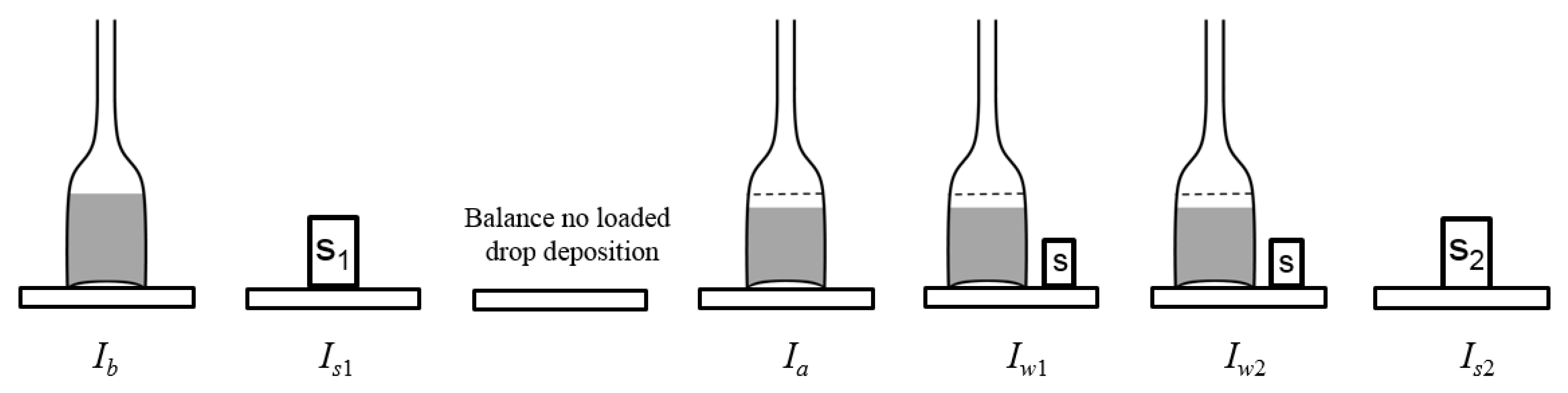
2.1. Mass Measurement
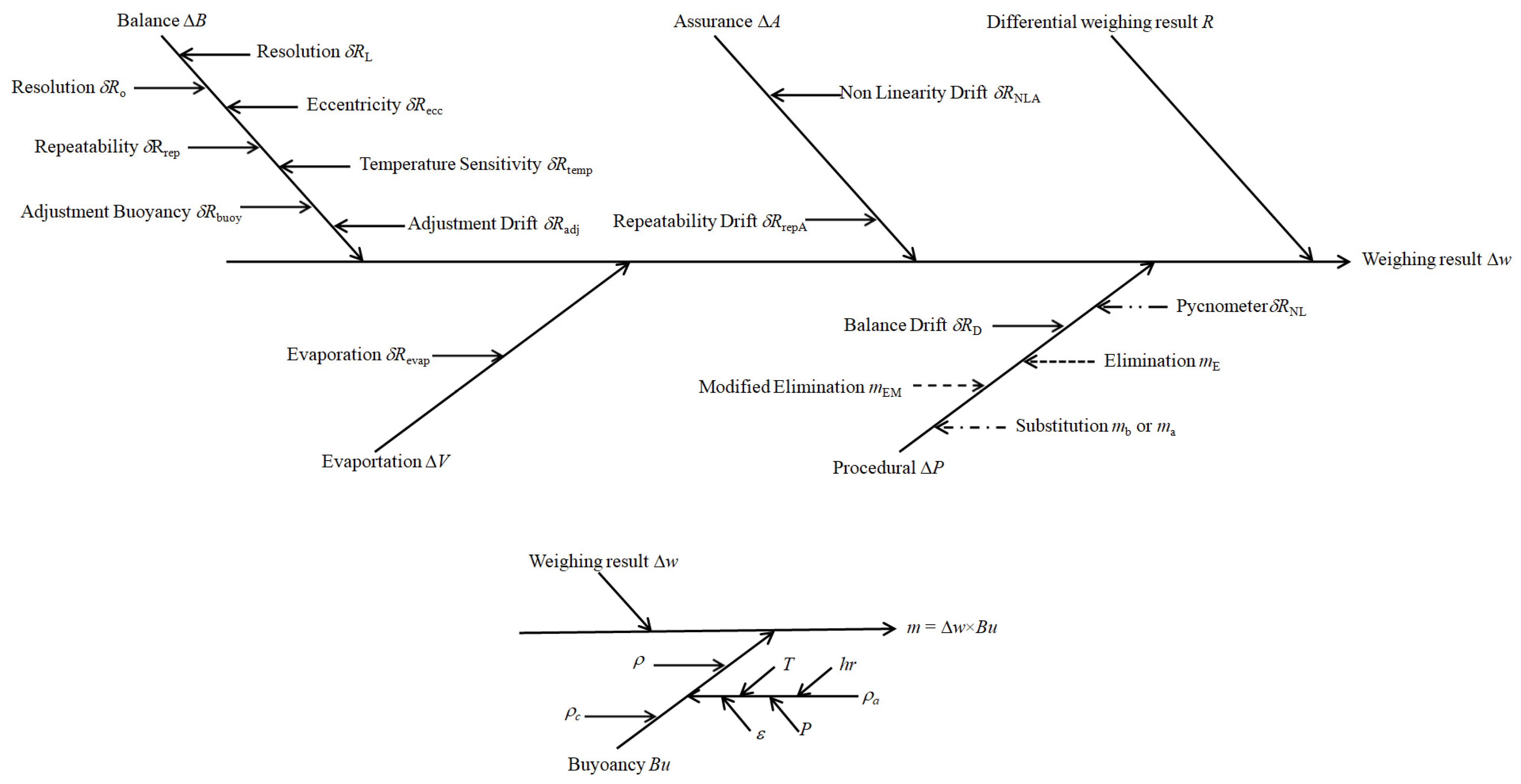
2.2. Uncertainty Evaluation for Mass Measurement
2.3. Uncertainty Evaluation for Buoyancy
2.4. Uncertainty Evaluation for Weighing
2.4.1. Resolution
2.4.2. Eccentricity
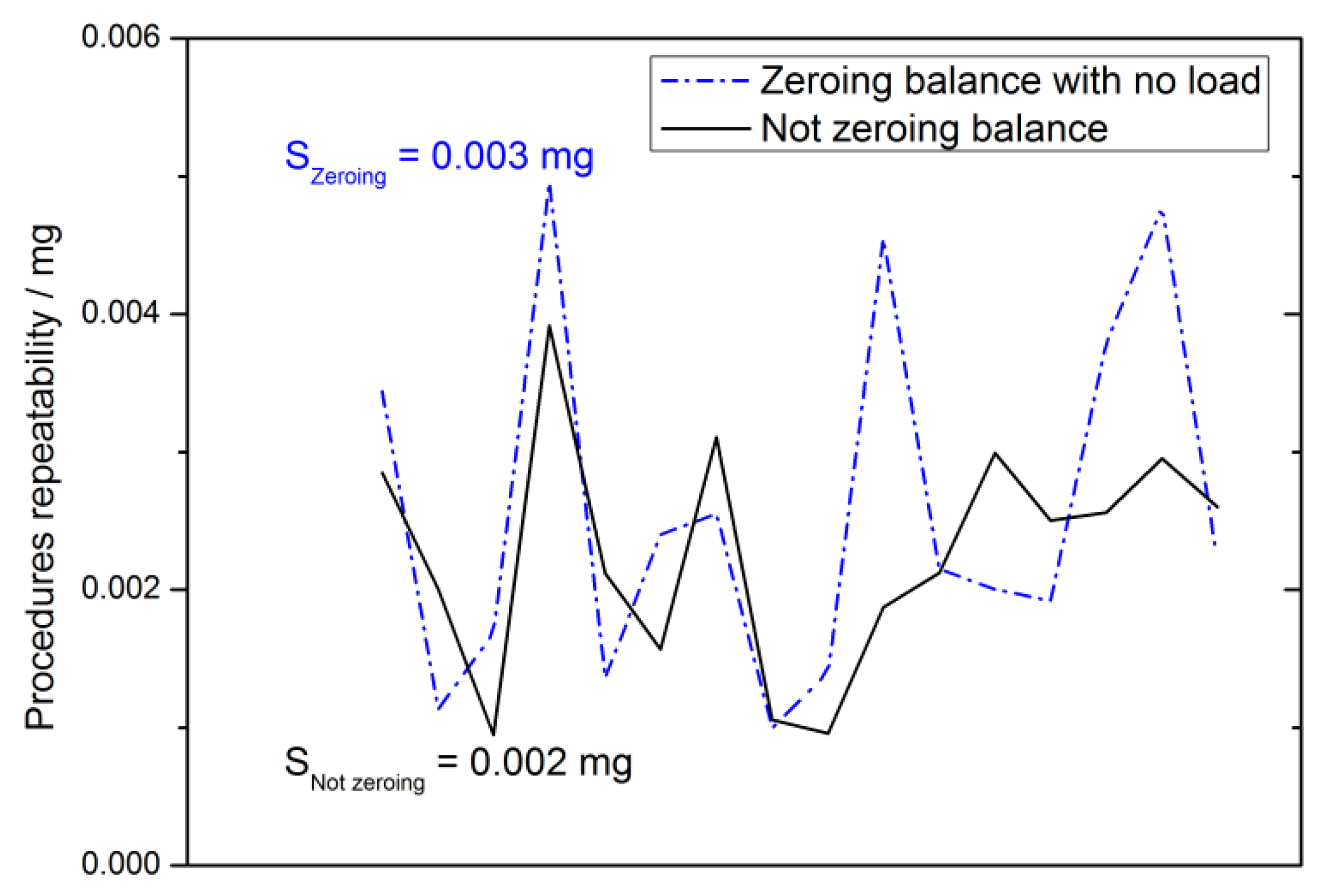
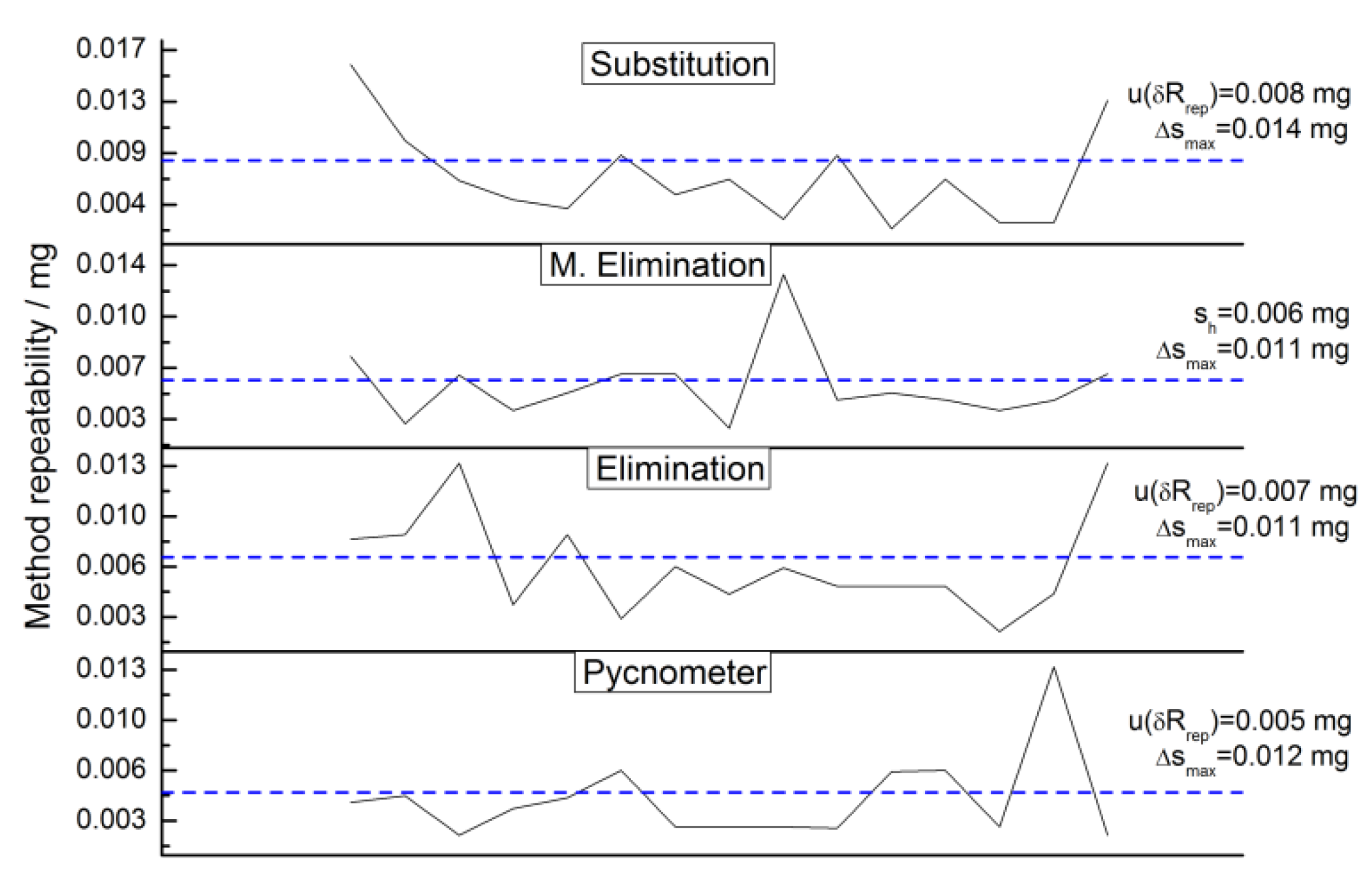
2.4.3. Repeatability
2.4.4. Temperature Sensitivity
2.4.5. Buoyancy Adjustment
2.4.6. Drift Adjustment
2.4.7. Evaporation
2.4.8. Non-Linearity
2.4.9. Balance Drift
2.4.10. Standard Weights Mass
2.4.11. Non-Linearity Drift
2.4.12. Repeatability Uncertainty Estimate
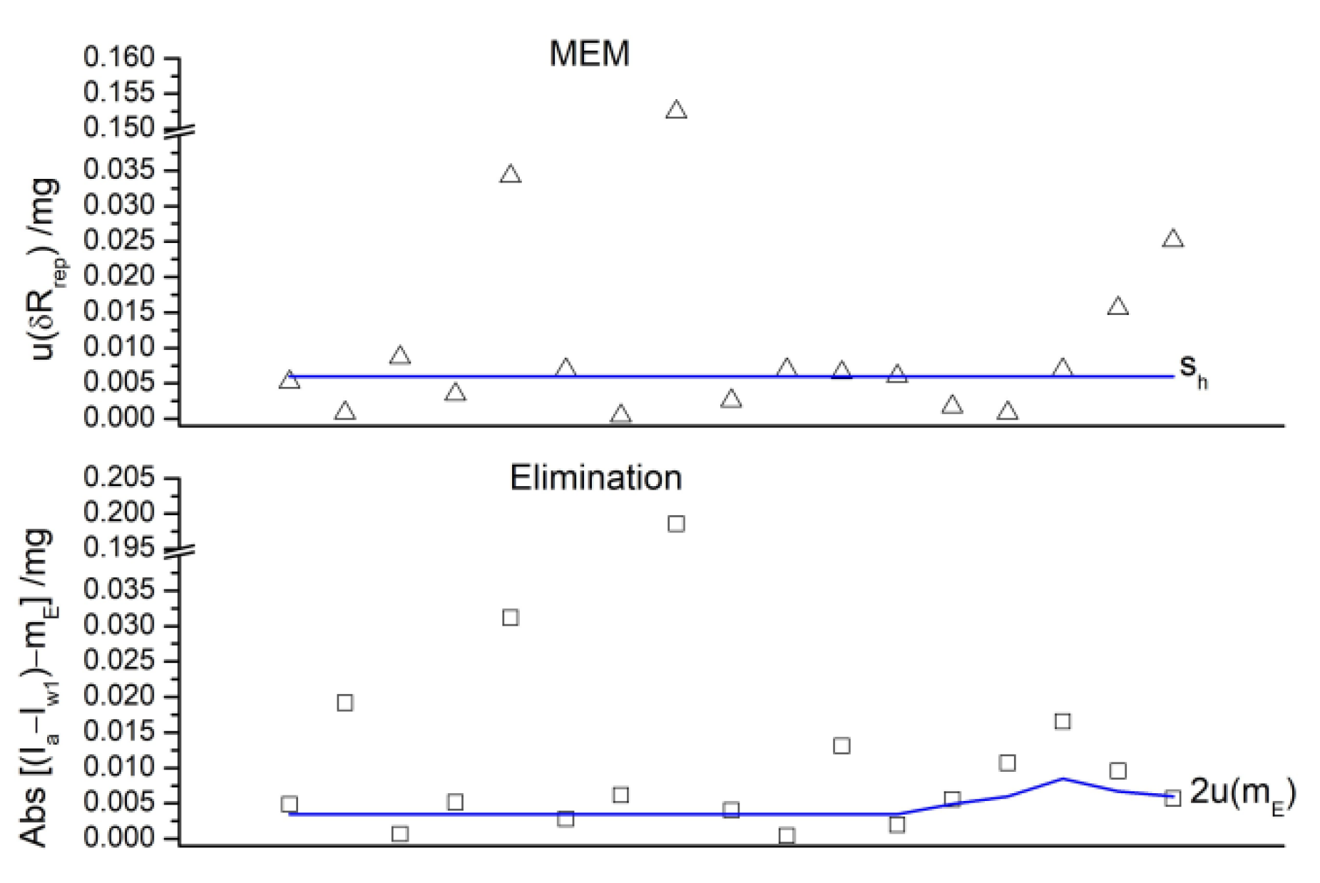
2.5. Check for Non-Expected Effects
3. Materials and Methods
3.1. Experimental Set Up
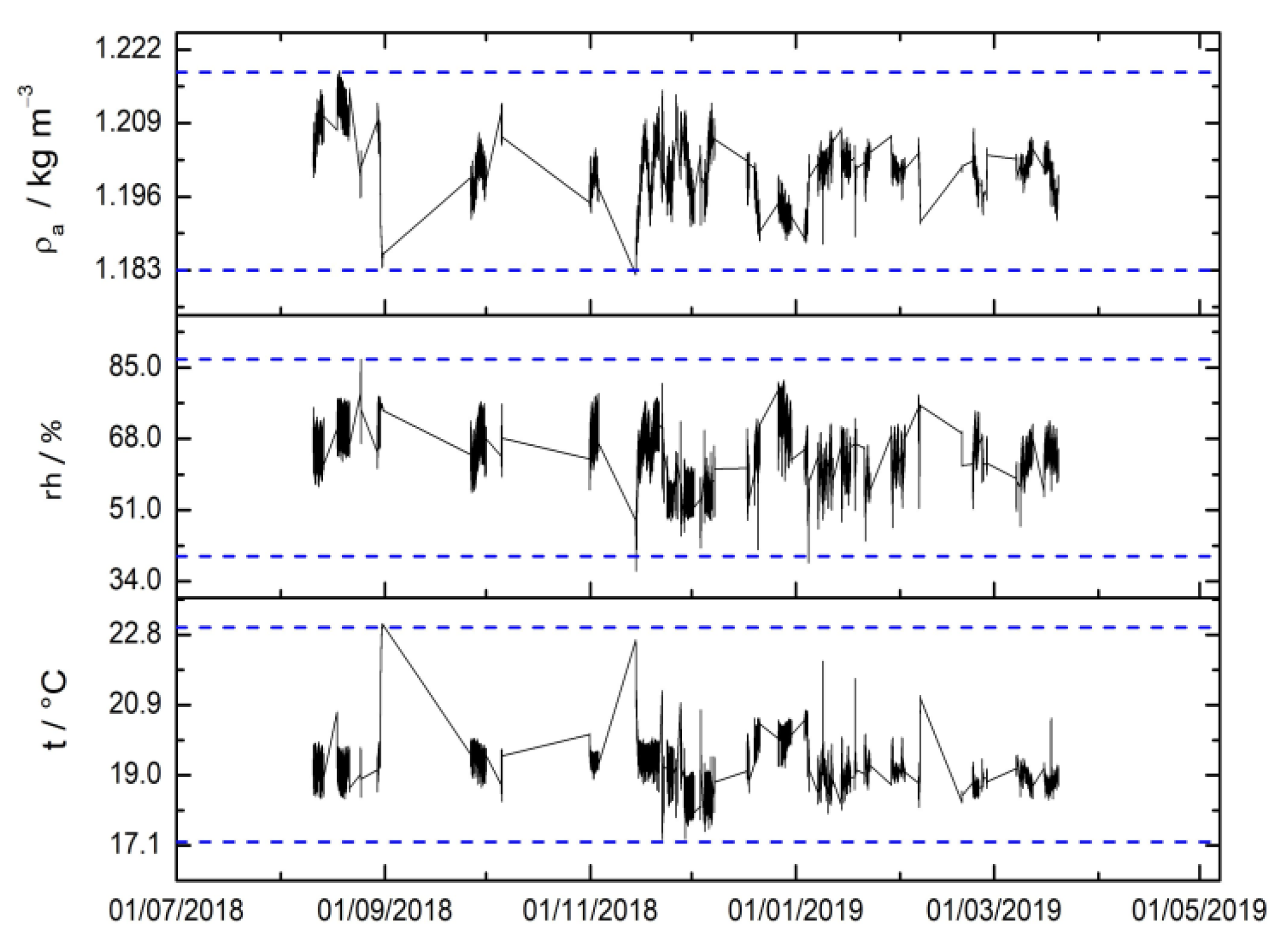
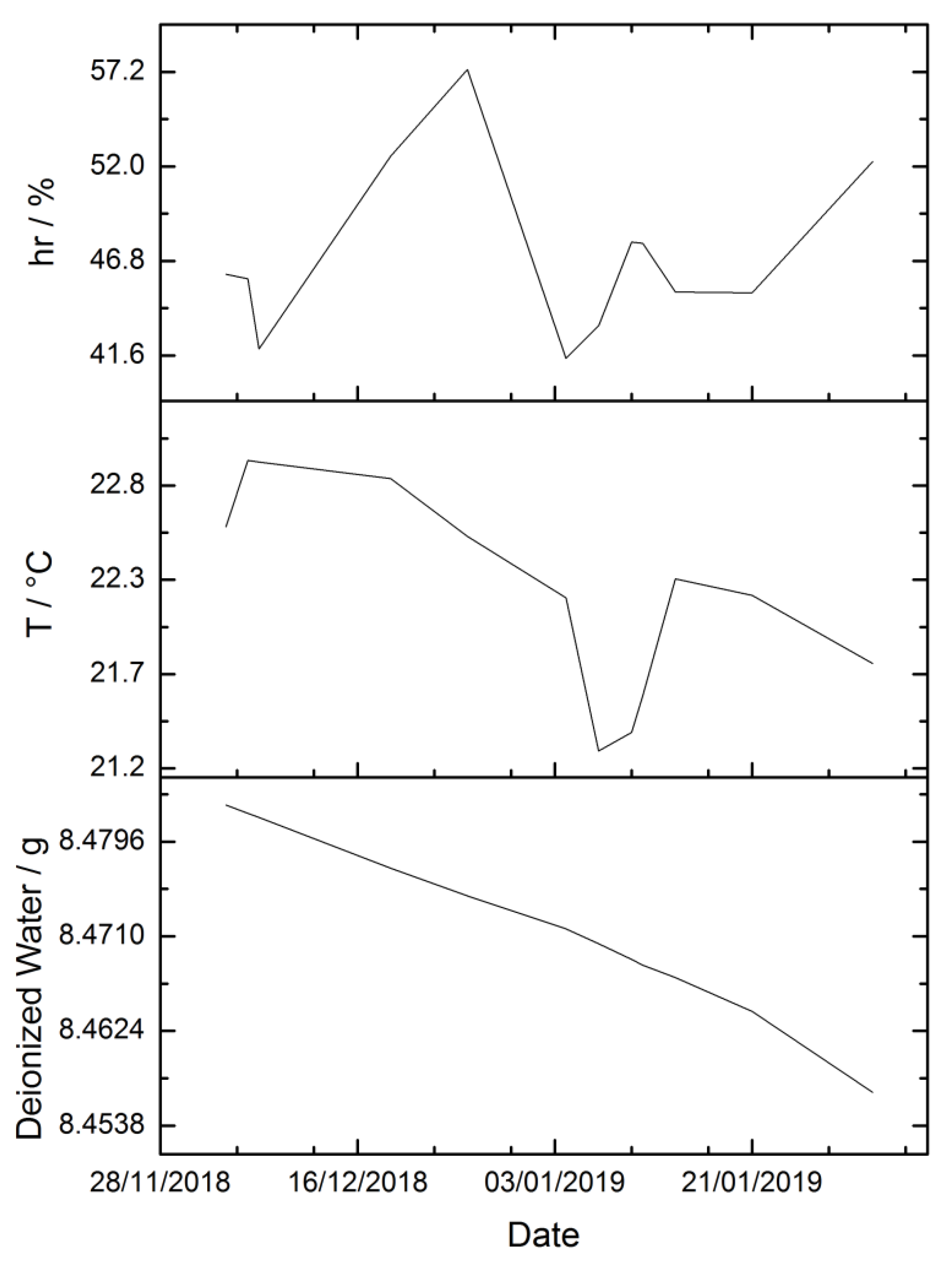
3.2. Environmental Parameters
3.3. Radionuclide Solution Parameters
3.3.1. Density
3.3.2. Evaporation
3.4. Balance Parameters
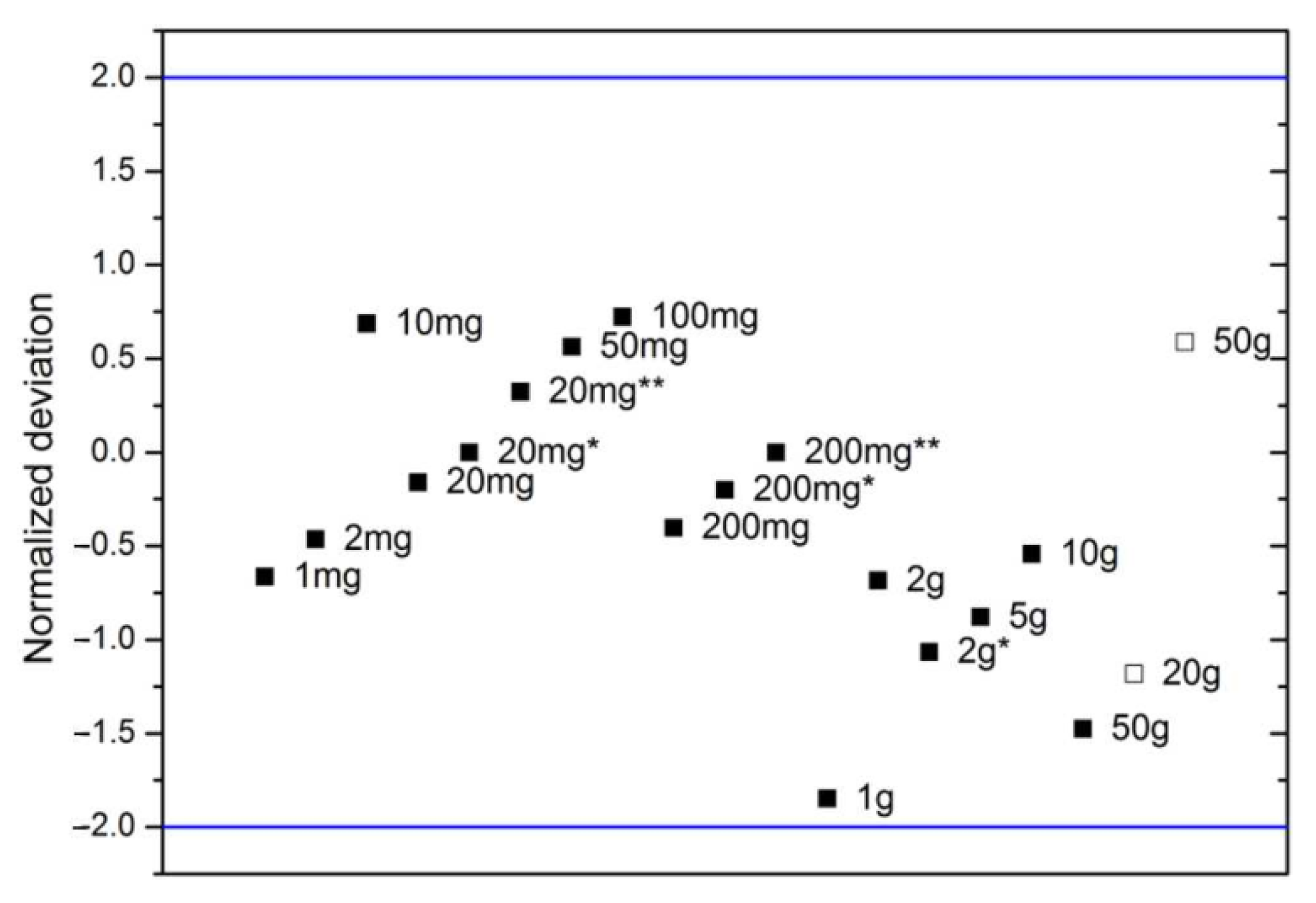
3.4.1. Standard Weights
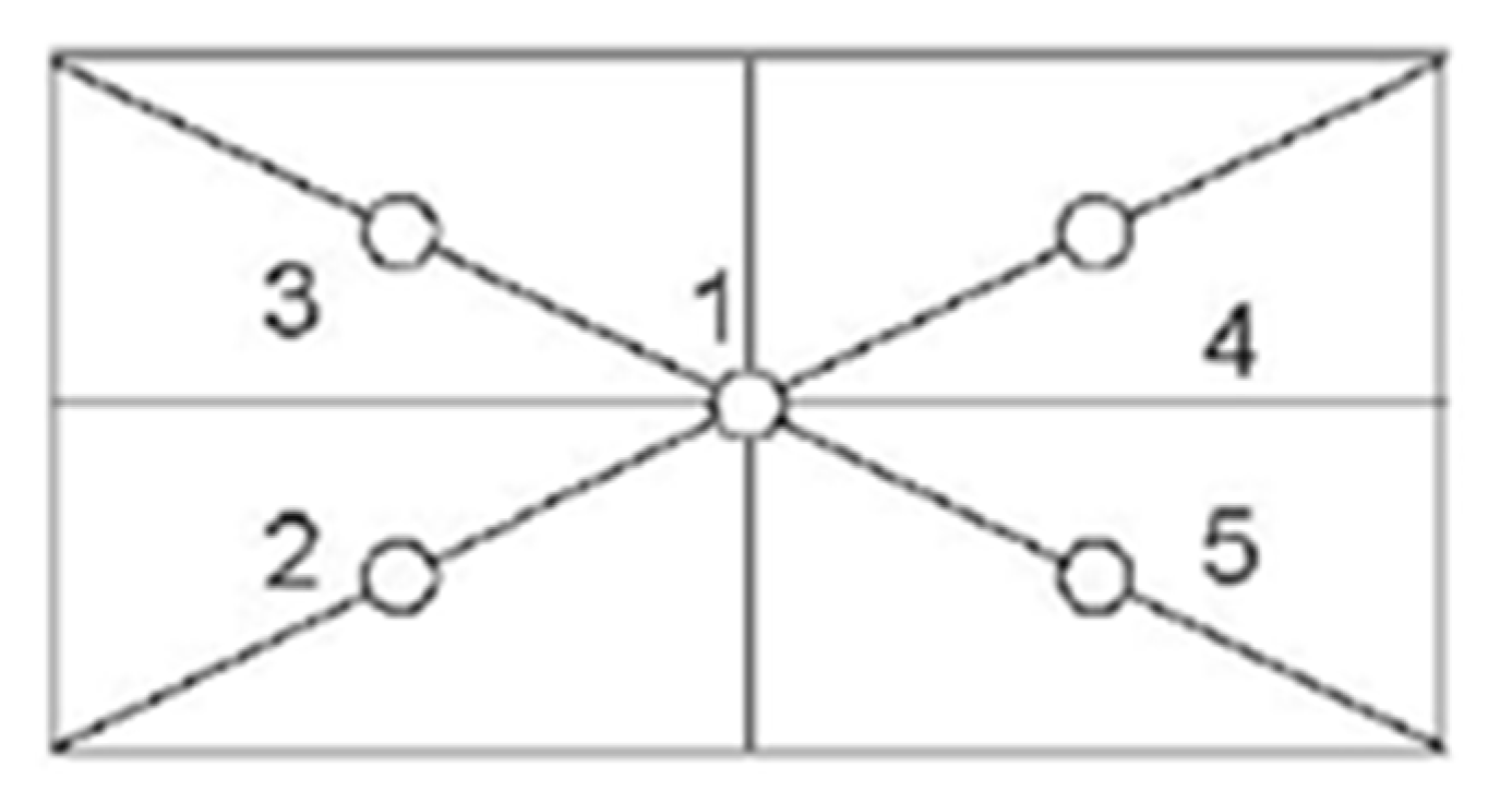
3.4.2. Eccentricity Test
3.4.3. Non-Linearity Checks
3.4.4. Balance Drift Avoiding Procedures
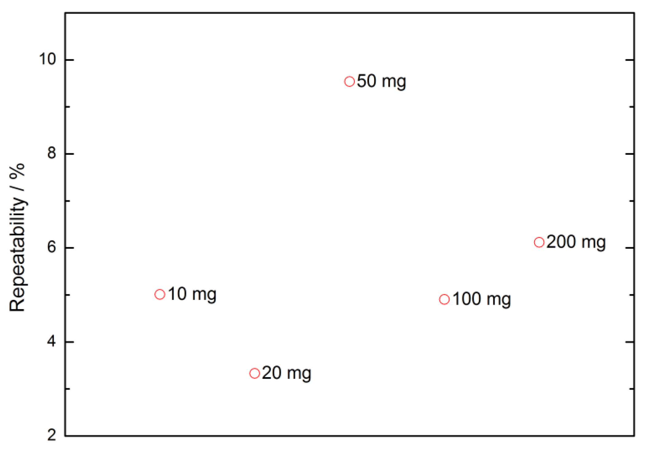
3.4.5. Weighing Methods Repeatability
4. Measurement
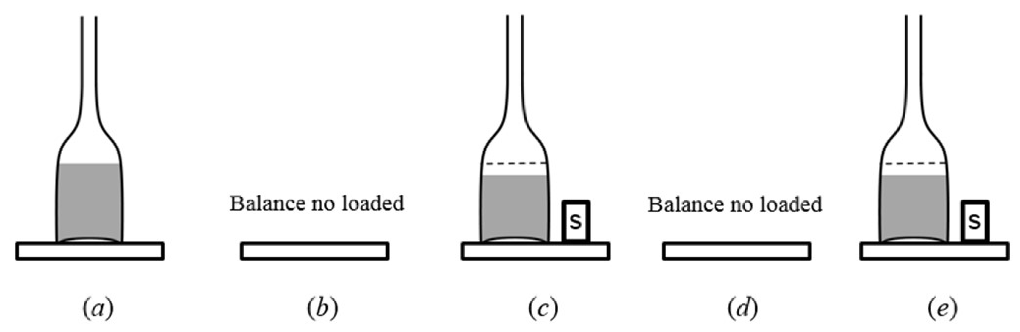
4.1. Weighing
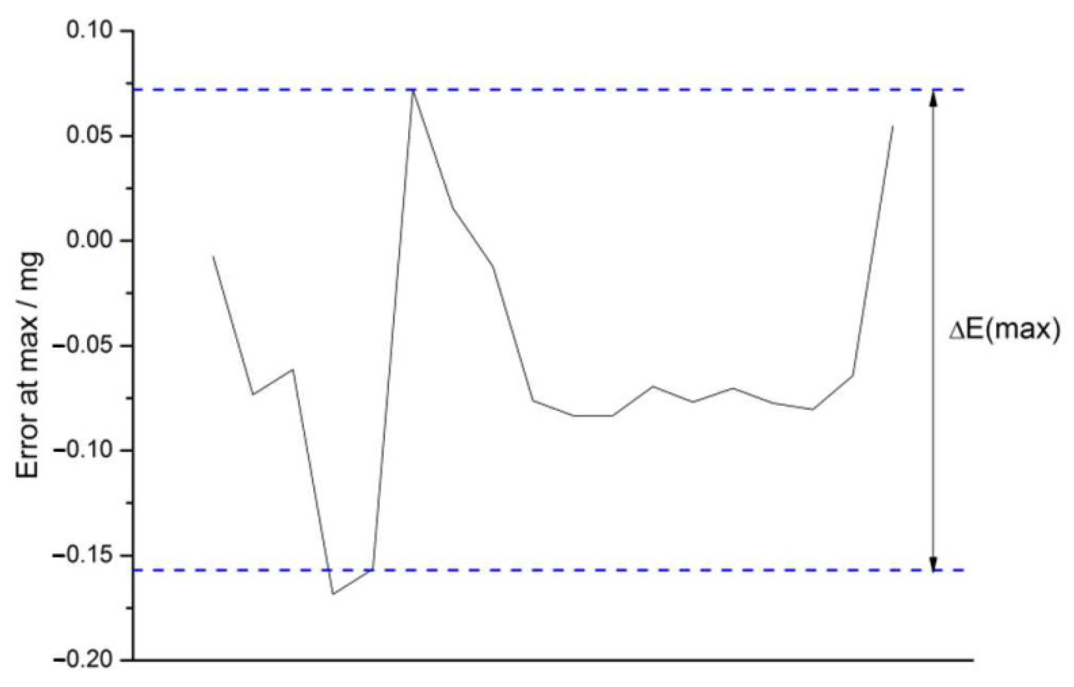
4.2. Checks for Errors
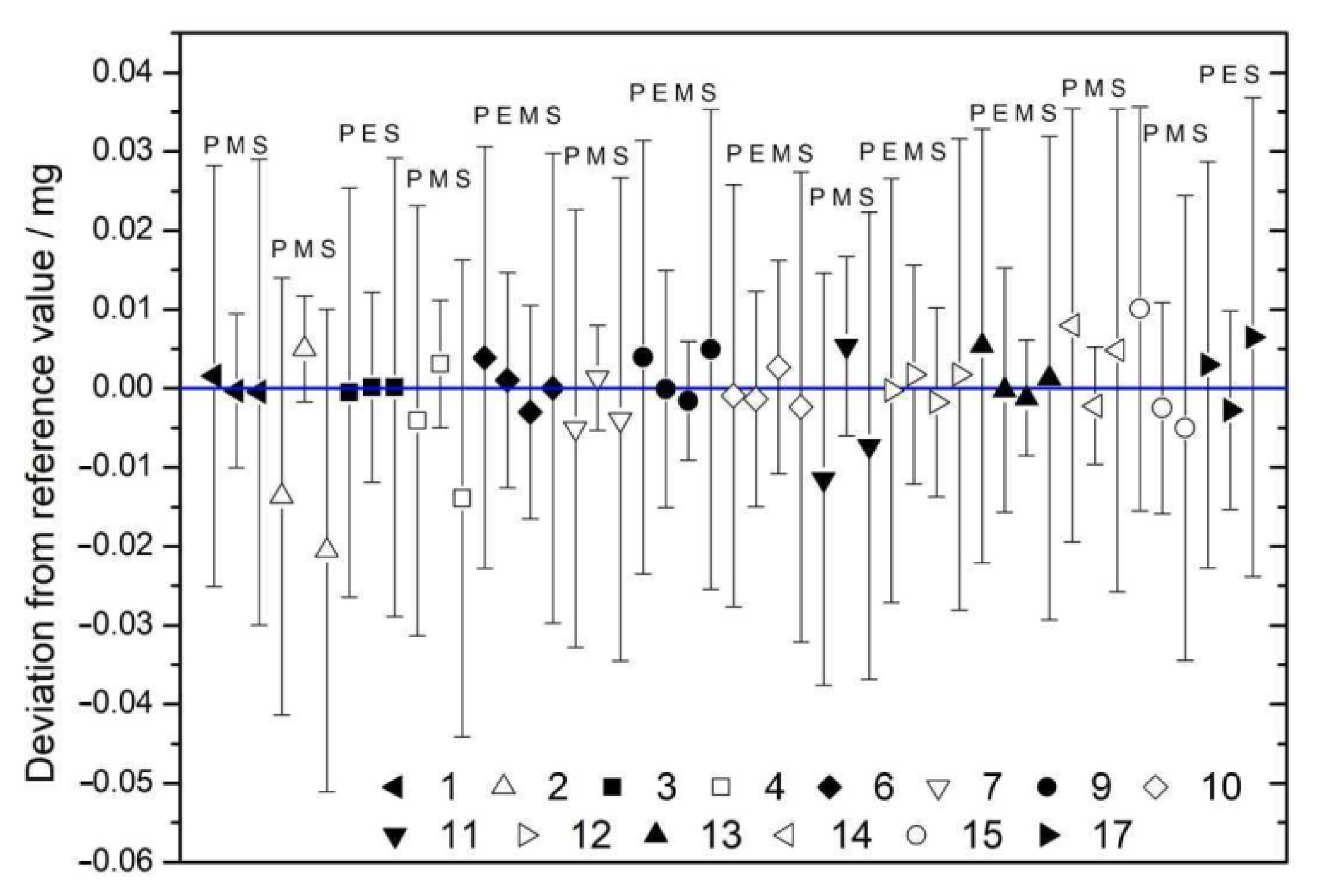
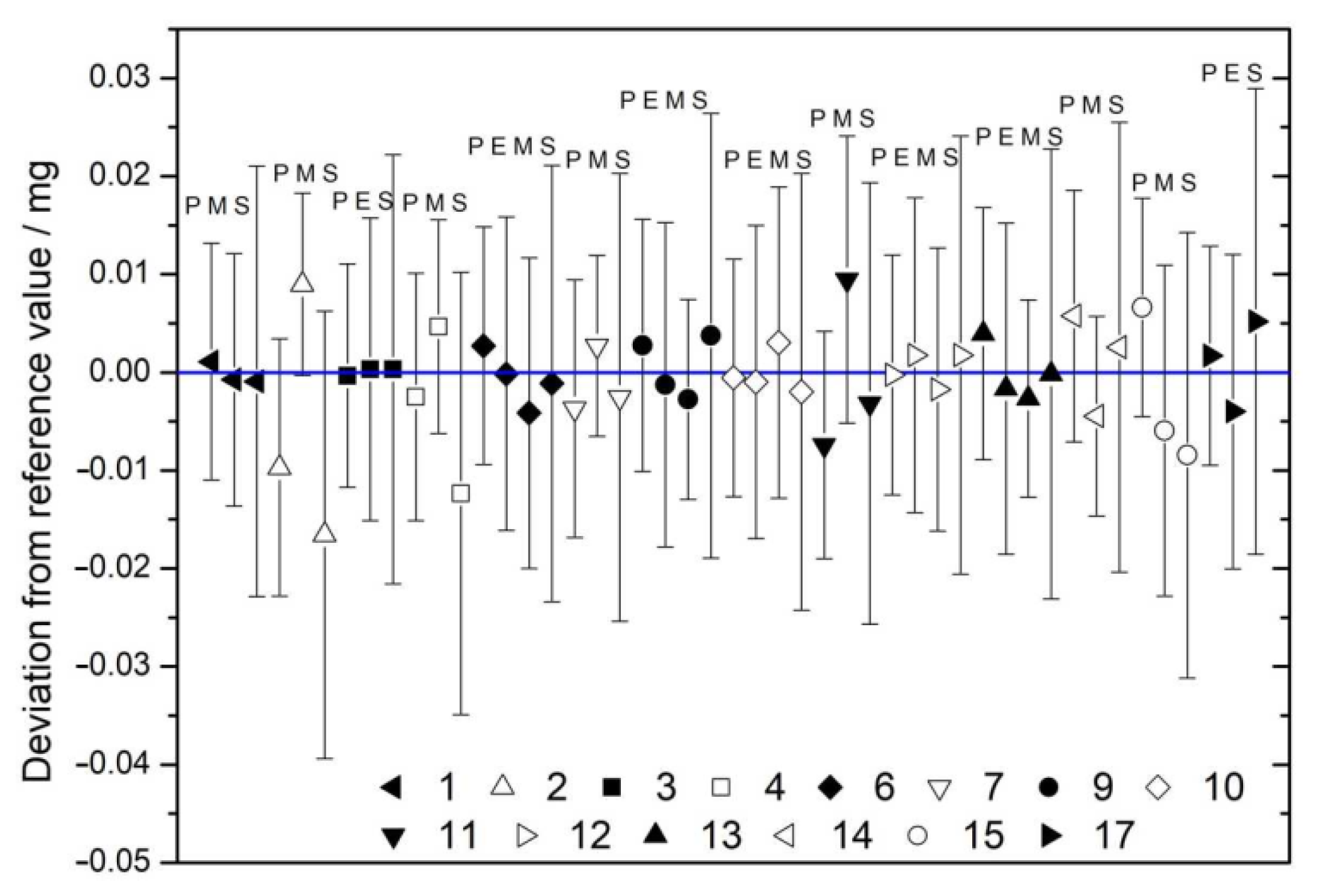
4.3. Mass Comparison
5. Conclusions
Author Contributions
Funding
Informed Consent Statement
Acknowledgments
Conflicts of Interest
References
- Campion, P.J. Procedures for Accurately Diluting and Dispensing Radioactive Solutions; Monographie BIPM-l: Sèvres, France, 1975. [Google Scholar]
- Sibbens, G.; Altzitzoglou, T. Preparation of radioactive sources for radionuclide metrology. Metrologia 2007, 44, S71–S78. [Google Scholar] [CrossRef]
- Thiam, C.; Bobin, C.; Maringer, F.; Peyres, V.; Pommé, S. Assessment of the uncertainty budget associated with 4πγ counting. Metrologia 2015, 52, S97. [Google Scholar] [CrossRef]
- Bailat, C.J.; Keightley, J.; Nedjadi, Y.; Mo, L.; Ratel, G.; Michotte, C.; Roteta, M. International comparison CCRI(II)-S7 on the analysis of uncertainty budgets for 4πβγ coincidence counting. Metrologia 2014, 51, 06018. [Google Scholar] [CrossRef]
- Campion, P.; Dale, J.; Williams, A. A study of weighing techniques used in radionuclide standardization. Nucl. Instrum. Methods 1964, 31, 253–261. [Google Scholar] [CrossRef]
- van der Eijk, W.; Moret, H. Precise determination of drop weights. In Standardization of Radionuclides, Proceedings of A Symposium on Standardization of Radionuclides, Vienna, Austria, 10–14 October 1967; International Atomic Energy Agency: Vienna, Austria, 1967; p. 529. [Google Scholar]
- Van Der Eijk, W.; Vaninbroukx, R. Sampling and dilution problems in radioactivity measurements. Nucl. Instrum. Methods 1972, 102, 581–587. [Google Scholar] [CrossRef]
- Pommé, S. When the model doesn’t cover reality: Examples from radionuclide metrology. Metrologia 2016, 53, S55–S64. [Google Scholar] [CrossRef][Green Version]
- Le Gallic, Y. Problems in microweighing. Nucl. Instrum. Methods 1973, 112, 333–341. [Google Scholar] [CrossRef]
- Lourenço, V.; Bobin, C. Weighing uncertainties in quantitative source preparation for radionuclide metrology. Metrologia 2015, 52, S18–S29. [Google Scholar] [CrossRef]
- The CIPM MRA Database (KCDB) CCRI(II)-S7 Technical Protocol. Available online: https://www.bipm.org/kcdb/comparison?id=1417 (accessed on 18 August 2022).
- ISO/IEC 17025; General Requirements for the Competence of Testing and Calibration Laboratories. International Organization for Standardization: Geneva, Switzerland. Available online: https://en.wikipedia.org/wiki/ISO/IEC_17025 (accessed on 22 August 2022).
- Cacais, F.L.; Delgado, J.U.; Loayza, V.M.; Rangel, J.A. Bayesian estimation of the relative deviations between activities in the radionuclide standardization. Braz. J. Radiat. Sci. 2019, 7, 1–14. [Google Scholar] [CrossRef]
- Cacais, F.L.; Delgado, J.U.; Loayza, V.M. Uncertainty evaluation of a modified elimination weighing for source preparation. J. Phys. Conf. Ser. 2018, 975, 012057. [Google Scholar] [CrossRef]
- Cacais, F.L.; Delgado, J.U.; Loayza, V.M.; A Rangel, J. Comparison between three weighing methods for source preparation in radionuclide metrology. J. Phys. Conf. Ser. 2021, 1826, 012038. [Google Scholar] [CrossRef]
- Fitzgerald, R.; Bailat, C.; Bobin, C.; Keightley, J. Uncertainties in 4πβ–γ coincidence counting. Metrologia 2015, 52, S86–S96. [Google Scholar] [CrossRef]
- CIPM Mutual Recognition Arrangement (CIPM MRA) CMC Approval Process. Available online: https://www.bipm.org/en/cipm-mra/approval-process.html (accessed on 18 August 2022).
- Cacais, F.L.; Delgado, J.U.; Loayza, V.M. Taking degrees of freedom from uncertainty into minimum weight estimate for analytical balances. J. Phys. Conf. Ser. 2018, 1044, 012063. [Google Scholar] [CrossRef]
- Reichmuth, A. Weighing Small Samples on Laboratory Balances. In Transverse Disciplines in Metrology, Proceedings of the 13th International Metrology Congress, Lille, France, 1 May 2007; Wiley: Hoboken, NJ, USA, 2007; pp. 641–656. [Google Scholar]
- Glaser, M. Magnetic interactions between weights and weighing instruments. Meas. Sci. Technol. 2001, 12, 709–715. [Google Scholar] [CrossRef]
- OIML R111; Weights of Classes E1, E2, F1, F2, M1, M1-2, M2, M2-3, M3 Part 1: Metrological and Technical Requirements. International Organization of Legal Metrology: Paris, France, 2014. Available online: https://www.oiml.org/en/files/pdf_r/r111-p-e04.pdf (accessed on 18 August 2022).
- Fritsch, K. GWP®—The Science-Based Global Standard for Efficient Lifecycle Management of Weighing Instruments. NCSLI Meas. 2013, 8, 60–69. [Google Scholar] [CrossRef]
- ISO 7870; Control Charts Series. International Organization for Standardization: Geneva, Switzerland, 2014.
- Euramet Calibration Guide No.18 Guidelines on the Calibration of Non-Automatic Weighing Instruments. Version 4.0. 2015. Available online: https://www.euramet.org/Media/docs/Publications/calguides/I-CAL-GUI-018_Calibration_Guide_No._18_web.pdf (accessed on 18 August 2022).
- OIML D28; Conventional Value of the Result of Weighing in Air. International Organization of Legal Metrology: Paris, France, 2004. Available online: https://www.oiml.org/en/files/pdf_d/d028-e04.pdf (accessed on 18 August 2022).
- Picard, A.; Davis, R.S.; Gläser, M.; Fujii, K. Revised formula for the density of moist air (CIPM-2007). Metrologia 2008, 45, 149–155. [Google Scholar] [CrossRef]
- JCGM 100:2008; Evaluation of Measurement Data—Guide to the Expression of Uncertainty in Measurement. Joint Committee for Guides in Metrology: Sèvres, France, 2008. Available online: https://www.bipm.org/utils/common/documents/jcgm/JCGM_100_2008_E.pdf (accessed on 1 May 2022).
- Wunderli, S.; Fortunato, G.; Reichmuth, A.; Richard, P. Uncertainty evaluation of mass values determined by electronic balances in analytical chemistry: A new method to correct for air buoyancy. Anal. Bioanal. Chem. 2003, 376, 384–391. [Google Scholar] [CrossRef]
- Merritt, J.S. Present status in quantitative source preparation. Nucl. Instrum. Methods 1973, 112, 325–332. [Google Scholar] [CrossRef]
- Reichmuth, A. Non-Linearity of Laboratory Balances and Its Impact on Uncertainty. In Proceedings of the NCSL International 2000 Workshop and Symposium, Toronto, ON, Canada, 16–20 July 2000. [Google Scholar]
- ISO 10012; Measurement Management Systems—Requirements for Measurement Processes and Measuring Equipment. International Organization for Standardization: Geneva, Switzerland, 2003.
- Nielsen, L. Evaluation of mass measurements in accordance with the GUM. Metrologia 2014, 51, S183–S190. [Google Scholar] [CrossRef]
- JCGM 101:2008; Evaluation of Measurement Data—Supplement 1 to the ‘Guide to the Expression of Uncertainty in Measurement’—Propagation of Distributions Using a Monte Carlo Method. Joint Committee for Guides in Metrology: Sèvres, France, 2008. Available online: https://www.bipm.org/utils/common/documents/jcgm/JCGM_101_2008_E.pdf (accessed on 18 August 2022).
- Malengo, A. Buoyancy effects and correlations in calibration and use of electronic balances. Metrologia 2014, 51, 441–451. [Google Scholar] [CrossRef]
- OIML R76; Non-Automatic Weighing Instruments Part1: Metrological Requirements—Tests. International Organization of Legal Metrology: Paris, France, 2006. Available online: https://www.oiml.org/en/files/pdf_r/r076-p-e06.pdf (accessed on 18 August 2022).
- JCGM 200:2012; International Vocabulary of Metrology—Basic and General Concepts and Associated Terms (VIM 3rd ed.). Joint Committee for Guides in Metrology: Sèvres, France, 2012. Available online: http://www.bipm.org/utils/common/documents/jcgm/JCGM_200_2012.pdf (accessed on 1 May 2022).
- Reichmuth, A. Weighing accuracy with laboratory balances. In Transverse Disciplines in Metrology, Proceedings of the 13th International Metrology Congress, Lille, France, 1 May 2007; Wiley: Hoboken, NJ, USA, 2007; p. 38. [Google Scholar]
- Migon, H.; Gamerman, D. Statistical Inference: An Integrated Approach; Arnold Publishers: London, UK, 1999. [Google Scholar]
- Fritsch, K. Personal Communication; Mettler-Toledo GmbH: Greifensee, Switzerland, 2017. [Google Scholar]
- Janβen, H. Uncertainties in Weighing; Presentation; VERMI Young Researchers Workshop: Geel, Belgium, 2004. [Google Scholar]
- Clark, J.P.; Shull, H. Reproducibility: A Major Source of Uncertainty in Weighing; Report in Conjunction with Contract No.DE-AC09-96SR18500 with the U.S. Department of Energy; U.S. Department of Energy: Washington, DC, USA, 2001.
- Arduino Reference. Available online: https://www.arduino.cc/ (accessed on 7 May 2019).
- Mettler-Toledo. Excellence Plus Analytical Balances XP Models, Operating Instructions. Available online: https://www.mt.com/dam/P5/labtec/02_Analytical_Balances/03_XP/03_Documentations/03_Operating_Instructions/OI_XP_Analytical_Part_1_EN.pdf (accessed on 18 August 2022).
- BOSCH. Humidity Sensor BME280. Available online: https://www.bosch-sensortec.com/products/environmental-sensors/humidity-sensors-bme280/ (accessed on 18 August 2022).
- Arduino. Temperature Monitoring with DHT22. Available online: https://create.arduino.cc/projecthub/projects/tags/dht22 (accessed on 18 August 2022).
- Arduino. BMP180 Interfacing with Arduino in Depth. Available online: https://create.arduino.cc/projecthub/weargenius/bmp180-interfacing-with-arduino-in-depth-68595b (accessed on 18 August 2022).
- Mettler-Toledo. DA-310M Density Meter. Available online: https://www.mt.com/au/en/home/phased_out_products/PhaseOut_Ana/DA310M.html (accessed on 18 August 2022).
- NCRP-Report-58—Techniques for the Preparation of Standard Sources for Radioactivity Measurements. In A Handbook of Radioactivity Measurements Procedures (Report 58), 2nd ed.; National Council on Radiation Protection and Measurements: Bethesda, MD, USA, 1985.
- Letho, J.; Hou, X. Chemistry and Analysis of Radionuclides. In Laboratory Techniques and Methodology; Wiley: Weinheim, Germany, 2011. [Google Scholar]
- Rizzuto, A.M.; Cheng, E.S.; Lam, R.K.; Saykally, R.J. Surprising Effects of Hydrochloric Acid on the Water Evaporation Coefficient Observed by Raman Thermometry. J. Phys. Chem. C 2017, 121, 4420–4425. [Google Scholar] [CrossRef]
- Nielsen, L. Identification and Handling of Discrepant Measurements in Key Comparisons; Technical Report DFM-02-R28; Danish Institute of Fundamental Metrology Denmark: Hørsholm, Denmark, 2002. [Google Scholar]
- Reichmuth, A. Non-Linearity of High Resolution Laboratory Balances; South Yorkshire Trading Standards Unit: Sheffield, UK, 2000. [Google Scholar]
- Mettler-Toledo AT/MT/UMT Balances Technical Specifications and Accessories. Available online: http://www.dragon.lv/exafs/equipment/at-mt-umt-tez-e-703466.pdf (accessed on 18 August 2022).
- Reichmuth, A.; Wunderli, S.; Weber, M.; Meyer, V.R. The Uncertainty of Weighing Data Obtained with Electronic Analytical Balances. Mikrochim. Acta 2004, 148, 133–141. [Google Scholar] [CrossRef]
- IAEA. Optimization of Radiation Protection in the Control of Occupational Exposure; Safety reports series No. 21; International Atomic Energy Agency: Vienna, Austria, 2002. [Google Scholar]
- Nielsen, L. Methods for the Evaluation of Key Comparisons; Euromet Mass & Related Quantities TC Meeting: Bern, Switzerland, 2003. [Google Scholar]
- Ratel, G.; Michotte, C.; Courte, S.; Kossert, K. Update of the BIPM Comparison BIPM.RI(II)-K1.Ho-166m Activity Measurements of the Radionuclide 166mHo for the PTB (Germany), with Linked Results for the EURAMET.RI(II)-K2.Ho-166m Comparison. Metrologia 2015, 52, 06006. [Google Scholar] [CrossRef][Green Version]
- Becerra, L.O.; Orys, M.; Chung, J.W.; Davidson, S.; Fuchs, P.; Jacques, C.; Jian, W.; Kubarych, Z.J.; Kumar, A.; Malengo, A.; et al. Final report on CCM.M-K4: Key comparison of 1 kg stainless steel mass standards. Metrologia 2014, 51, 07009. [Google Scholar] [CrossRef]
- Molloy, E.; Koo, A.; Hall, B.D.; Harding, R. The Statistical Power and Confidence of Some Key Comparison Analysis Methods to Correctly Identify Participant Biases. Metrology 2021, 1, 4. [Google Scholar] [CrossRef]


| Nominal Value | E ± U(k = 2)/µg |
|---|---|
| 1 mg | −2 ± 3 |
| 2 mg | −42 ± 3 |
| 10 mg | −14 ± 3 |
| 20 mg | −3 ± 3 |
| 20 mg * | −16 ± 3 |
| 20 mg ** | −327 ± 3 |
| 50 mg | 5802 ± 5 |
| 100 mg | −64 ± 5 |
| 200 mg | −8 ± 6 |
| 200 mg * | −3 ± 6 |
| 200 mg ** | −7 ± 6 |
| 1 g | −8166 ± 12 |
| 2 g | −13,455 ± 14 |
| 2 g * | −10,259 ± 14 |
| 5 g | −11,810 ± 20 |
| 10 g | −30 ± 20 |
| 50 g | −150 ± 30 |
| 20 g F1 | −73,810 ± 90 |
| 50 g F1 | −78,230 ± 120 |
| Sequence | Ib/g | Is1/g | Ia/g | Iw1/g | Iw2/g | Is2/g | p/hPa | hr/% | t/°C |
|---|---|---|---|---|---|---|---|---|---|
| 1 | 3.398445 | 3.381587 | 3.374228 | 3.393906 | 3.393900 | 3.381585 | 1011.4 | 47 | 20.7 |
| 2 | 3.410688 | 3.401258 | 3.396206 | 3.415860 | 3.415861 | 3.381578 | 1014.8 | 51 | 20.8 |
| 3 | 3.428561 | 3.401252 | 3.410686 | 3.430359 | 3.430369 | 3.381580 | 1015.2 | 52 | 20.9 |
| 4 | 3.319494 | 3.301197 | 3.293126 | 3.312796 | 3.312790 | 3.281514 | 1014.5 | 52 | 21.1 |
| 5 | 3.338214 | 3.301199 | 3.319625 | 3.339267 | 3.339228 | 3.281520 | 1014.5 | 50 | 21.0 |
| 6 | 3.308434 | 3.301200 | 3.272860 | 3.292536 | 3.292542 | 3.281523 | 1012.5 | 46 | 21.1 |
| 7 | 3.304571 | 3.301195 | 3.291554 | 3.311221 | 3.311221 | 3.281523 | 1012.5 | 46 | 21.0 |
| 8 | 3.328622 | 3.311501 | 3.315586 | 3.325373 | 3.325197 | 3.301516 | 1013.0 | 54 | 21.1 |
| 9 | 3.314540 | 3.311502 | 3.290265 | 3.310265 | 3.310269 | 3.291506 | 1012.9 | 52 | 21.3 |
| 10 | 3.290278 | 3.291508 | 3.279235 | 3.289221 | 3.289215 | 3.281521 | 1012.9 | 50 | 21.3 |
| 11 | 3.279235 | 3.291509 | 3.266612 | 3.276585 | 3.276577 | 3.281515 | 1013.0 | 51 | 21.4 |
| 12 | 3.558546 | 3.558315 | 3.536914 | 3.556909 | 3.556915 | 3.538320 | 1014.0 | 58 | 20.1 |
| 13 | 3.536926 | 3.534446 | 3.524990 | 3.536938 | 3.536941 | 3.522498 | 1013.9 | 57 | 20.4 |
| 14 | 3.378801 | 3.378300 | 3.353493 | 3.376457 | 3.376456 | 3.357314 | 1018.2 | 57 | 20.5 |
| 15 | 3.353494 | 3.334445 | 3.113683 | 3.353673 | 3.353667 | 3.114453 | 1018.6 | 58 | 20.3 |
| 16 | 3.775687 | 3.777316 | 3.709477 | 3.775274 | 3.775256 | 3.711492 | 1015.2 | 59 | 19.7 |
| 17 | 3.684177 | 3.681524 | 3.660887 | 3.683846 | 3.683875 | 3.660347 | 1015.4 | 58 | 19.6 |
| # | mb | ma | mE, mEM |
|---|---|---|---|
| 1 | 2 g *, 1 g, 200 mg, 200 mg * | mb | 20 mg ** |
| 2 | 2 g *, 1 g, 200 mg, 200 mg *, 20 mg ** | mb − 20 mg ** | 20 mg ** |
| 3 | 2 g *, 1 g, 200 mg, 200 mg *, 20 mg ** | mb − 20 mg ** | 20 mg ** |
| 4 | 2 g *, 1 g, 200 mg *, 100 mg, 20 mg ** | mb − 20 mg ** | 20 mg ** |
| 5 | 2 g *, 1 g, 200 mg, 200 mg *, 20 mg ** | mb − 20 mg ** | 20 mg ** |
| 6 | 2 g *, 1 g, 200 mg *, 100 mg, 20 mg ** | mb − 20 mg ** | 20 mg ** |
| 7 | 2 g *, 1 g, 200 mg, 200 mg *, 20 mg ** | mb − 20 mg ** | 20 mg ** |
| 8 | 2 g *, 1 g, 200 mg *, 100 mg, 20 mg, 10 mg | mb − 10 mg | 10 mg |
| 9 | 2 g *, 1 g, 200 mg *, 100 mg, 20 mg, 10 mg | mb − 20 mg | 20 mg |
| 10 | 2 g *, 1 g, 200 mg *, 100 mg, 20 mg, 10 mg | mb − 20 mg | 10 mg |
| 11 | 2 g *, 1 g, 200 mg *, 100 mg, 20 mg, 10 mg | mb − 20 mg − 10 mg + 20 mg * | 10 mg |
| 12 | 2 g *, 1 g, 200 mg, 200 mg *, 100 mg, 50 mg, 20 mg, 1 mg | mb − 20 mg | 20 mg |
| 13 | 2 g *, 1 g, 200 mg, 200 mg *, 100 mg, 20 mg *, 20 mg, 10 mg, 2 mg, 1 mg | mb − 10 mg − 2 mg | 10 mg, 2 mg |
| 14 | 2 g *, 1 g, 200 mg, 100 mg, 50 mg, 20 mg *, 20 mg, 1 mg | mb − 20 mg * − 1 mg | 20 mg, 2 mg, 1 mg |
| 15 | 2 g *, 1 g, 200 mg, 100 mg, 20 mg *, 20 mg, 10 mg, 2 mg, 1 mg | mb − 200 mg − 20 mg * | 200 mg, 20 mg *, 20 mg |
| 16 | 2 g *, 1 g, 200 mg, 200 mg *, 200 mg **, 100 mg, 50 mg, 20 mg *, 20 mg | mb − 50 mg − 20 mg + 10 mg | 50 mg, 10 mg |
| 17 | 2 g *, 1 g, 200 mg, 200 mg *, 200 mg **, 100 mg | mb − 100 mg + 50 mg + 20 mg + 2 mg + 1 mg | 20 mg, 2 mg, 1 mg |
| Pycnometer | Elimination | M. Elimination | Substitution | |||||||
|---|---|---|---|---|---|---|---|---|---|---|
| Before | After | |||||||||
| Quantity (X) | Value | u(X) | Value | u(X) | Value | u(X) | Value | u(X) | Value | u(X) |
| Resol at 0 | 0 | 0.0003 | 0 | 0.0003 | 0 | 0.0003 | 0 | 0.0003 | 0 | 0.0003 |
| Resol at L | 0 | 0.0003 | 0 | 0.0003 | 0 | 0.0003 | 0 | 0.0003 | 0 | 0.0003 |
| Eccentricity | 0 | 0.0000 | 0 | 0.0000 | 0 | 0.0000 | 0 | 0.0000 | 0 | 0.0000 |
| Repeatability | 0 | 0.0050 | 0 | 0.0070 | 0 | 0.0061 | 0 | 0.0080 | 0 | 0.0080 |
| Temp sensit | 0 | 0.0000 | 0 | 0.0000 | 0 | 0.0000 | 0 | 0.0000 | 0 | 0.0000 |
| Adj buoy | 0 | 0.0001 | 0 | 0.0000 | 0 | 0.0000 | 0 | 0.0000 | 0 | 0.0000 |
| Adj drift | 0 | 0.0001 | 0 | 0.0000 | 0 | 0.0000 | 0 | 0.0000 | 0 | 0.0000 |
| Evaporation | 0 | 0.0021 | 0 | 0.0021 | 0 | 0.0021 | 0 | 0.0021 | 0 | 0.0021 |
| Balance drift | 0 | 0.0003 | 0 | 0.0003 | 0 | 0.0003 | 0 | 0.0003 | 0 | 0.0003 |
| Repeat drift | 0 | 0.0069 | 0 | 0.0064 | 0 | 0.0064 | 0 | 0.0081 | 0 | 0.0081 |
| Linearity | 0 | 0.0020 | not applicable | |||||||
| Linear drift | 0 | 0.0121 | ||||||||
| Std weight | 19.9970 | 0.0017 | 19.9970 | 0.0017 | 3558.2970 | 0.0113 | 3538.3000 | 0.0112 | ||
| Meth result | 21.6320 | 1.6370 | 1.6335 | 0.231 | −1.406 | |||||
| Weigh result | 21.6320 | 0.0151 | 21.6340 | 0.0098 | 21.6305 | 0.0092 | 3558.5280 | 0.0162 | 3536.8940 | 0.0161 |
| Cov/mg2 | not applicable | 0.0001 | ||||||||
| Bu = 1.00105 | u(Bu) = 0.00002 | |||||||||
| Drop mass | 21.655 | 0.015 | 21.657 | 0.010 | 21.653 | 0.009 | 21.657 | 0.016 | ||
| Rel uncert | 0.07% | 0.05% | 0.04% | 0.08% | ||||||
| # | mPyc | mElim | mMEM | mSubs | mRV |
|---|---|---|---|---|---|
| 1 | 24.242 ± 0.015 | 24.240 ± 0.009 | 24.240 ± 0.016 | 24.241 ± 0.007 | |
| 2 | 14.497 ± 0.015 | 14.516 ± 0.007 | 14.490 ± 0.016 | 14.511 ± 0.006 | |
| 3 | 17.894 ± 0.015 | 17.894 ± 0.010 | 17.894 ± 0.016 | 17.894 ± 0.008 | |
| 4 | 26.396 ± 0.015 | 26.403 ± 0.008 | 26.386 ± 0.016 | 26.400 ± 0.007 | |
| 6 | 35.611 ± 0.015 | 35.608 ± 0.010 | 35.604 ± 0.010 | 35.607 ± 0.016 | 35.607 ± 0.007 |
| 7 | 13.030 ± 0.015 | 13.037 ± 0.007 | 13.031 ± 0.016 | 13.035 ± 0.006 | |
| 9 | 24.300 ± 0.015 | 24.296 ± 0.010 | 24.294 ± 0.007 | 24.301 ± 0.016 | 24.296 ± 0.006 |
| 10 | 11.055 ± 0.015 | 11.054 ± 0.010 | 11.058 ± 0.010 | 11.053 ± 0.016 | 11.055 ± 0.007 |
| 11 | 12.636 ± 0.015 | 12.653 ± 0.010 | 12.640 ± 0.017 | 12.648 ± 0.008 | |
| 12 | 21.655 ± 0.015 | 21.657 ± 0.010 | 21.653 ± 0.009 | 21.657 ± 0.016 | 21.655 ± 0.007 |
| 13 | 11.949 ± 0.015 | 11.943 ± 0.010 | 11.942 ± 0.007 | 11.945 ± 0.017 | 11.944 ± 0.006 |
| 14 | 25.335 ± 0.015 | 25.324 ± 0.007 | 25.331 ± 0.017 | 25.327 ± 0.006 | |
| 15 | 240.063 ± 0.016 | 240.050 ± 0.011 | 240.048 ± 0.017 | 240.053 ± 0.009 | |
| 17 | 23.314 ± 0.015 | 23.308 ± 0.010 | 23.317 ± 0.017 | 23.311 ± 0.008 |
Publisher’s Note: MDPI stays neutral with regard to jurisdictional claims in published maps and institutional affiliations. |
© 2022 by the authors. Licensee MDPI, Basel, Switzerland. This article is an open access article distributed under the terms and conditions of the Creative Commons Attribution (CC BY) license (https://creativecommons.org/licenses/by/4.0/).
Share and Cite
Cacais, F.; Delgado, J.U.; Loayza, V.; Rangel, J. In Situ Validation Methodology for Weighing Methods Used in Preparing of Standardized Sources for Radionuclide Metrology. Metrology 2022, 2, 446-478. https://doi.org/10.3390/metrology2040027
Cacais F, Delgado JU, Loayza V, Rangel J. In Situ Validation Methodology for Weighing Methods Used in Preparing of Standardized Sources for Radionuclide Metrology. Metrology. 2022; 2(4):446-478. https://doi.org/10.3390/metrology2040027
Chicago/Turabian StyleCacais, Fabio, José Ubiratan Delgado, Victor Loayza, and Johnny Rangel. 2022. "In Situ Validation Methodology for Weighing Methods Used in Preparing of Standardized Sources for Radionuclide Metrology" Metrology 2, no. 4: 446-478. https://doi.org/10.3390/metrology2040027
APA StyleCacais, F., Delgado, J. U., Loayza, V., & Rangel, J. (2022). In Situ Validation Methodology for Weighing Methods Used in Preparing of Standardized Sources for Radionuclide Metrology. Metrology, 2(4), 446-478. https://doi.org/10.3390/metrology2040027