A General Mathematical Approach Based on the Possibility Theory for Handling Measurement Results and All Uncertainties

Abstract

The concept of measurement uncertainty was introduced in the 1990s by the “Guide to the expression of uncertainty in measurement”, known as GUM. The word uncertainty has a lexical meaning and reflects the lack of exact knowledge or lack of complete knowledge about the value of the measurand. Thanks to the suggestions in the GUM and following the mathematical probabilistic approaches therein proposed, an uncertainty value can be found and be associated to the measured value. In the last decades, however, other methods have been proposed in the literature, which try to encompass the definitions of the GUM, thus overcoming its limitations. Some of these methods are based on the possibility theory, such as the one known as the RFV method. The aim of this paper is to briefly recall the RFV method, starting from the very beginning and the initial motivations, and summarize in a unique paper the most relevant obtained results.

1. Background: The Concept of Measurement Uncertainty

In the 1990s, the “Guide to the expression of uncertainty in measurements”, known as GUM, introduced the concept of measurement uncertainty and provided some guidelines for its representation and propagation through the measurement function. In particular, the measurement uncertainty is defined as “a parameter, associated with the result of a measurement, that characterizes the dispersion of the values that could reasonably be attributed to the measurand” [1], as also recalled in [2].

This definition refers to a “dispersion of the values” because, as is widely known, when a quantity (the measurand) is measured more times, the measurement result generally varies, due to different contributions affecting the measurement procedure. This means that, because of the “dispersion of the values”, from a strict metrological point of view, the “true value” of the measurand cannot be known.

The uncertainty associated with a measured value has, therefore, the aim to provide information about how large this “dispersion of the values” is [1,2].

Therefore, from a strictly semantic point of view, it can be stated that the uncertainty value reflects the lack of exact knowledge or lack of complete knowledge about the value of the measurand. Hence, when one speaks about a measurement result, one always speaks about an incomplete information; this incomplete information must be somehow represented to provide validity of the measured value.

How can this representation be done? According to the GUM, the aim of the uncertainty evaluation is “to provide an interval about the measurement result that may be expected to encompass a large fraction of the distribution of values that could reasonably be attributed to the quantity subject to measurement” [1]. Furthermore, it clearly states that “the ideal method for evaluating and expressing measurement uncertainty should be capable of readily providing such an interval, in particular, one with a coverage probability or level of confidence that corresponds in a realistic way to that required” [1].

As stated above, the “dispersion of the values” is due to different contributions affecting the measurement procedure. In particular, in the “International vocabulary of metrology”, known as VIM [3], two contributions are defined: the random and the systematic contributions to uncertainty. (There is sometimes the mistake that the words random and systematic are substituted by the words “type A” and “type B”, defined in the GUM, respectively. However, “type A” and “type B” refer to methods of evaluation of the uncertainty contribution and not explicitly to the nature of the uncertainty contribution itself.)

The random contribution is defined as the “component of measurement error that in replicate measurements varies in an unpredictable manner” [3], while the systematic one is defined as the “Component of measurement error that in replicate measurements remains constant or varies in a predictable manner” [3]. Therefore, due to the random contributions to uncertainty, the dispersion of the measured values may define an interval around the mean (of the measured values), and this interval might be indeed the “interval about the measurement result that may be expected to encompass a large fraction of the distribution of values that could reasonably be attributed to the quantity subject to measurement” required by the GUM [1]. In Figure 1, the blue dot represents the measurand value, while the pink asterisk is the mean of the measured values, and the purple line represents the interval that includes all the measured values. It can be easily seen that the purple interval also encompasses the measurand value, as generally happens if a proper coverage factor is applied. However, if a systematic contribution also affects the measurement result, then the interval that includes all the measured values is shifted on the right/left with respect to the previous interval. The direction of right or left depends on whether the systematic effect is positive or negative, as shown with the blue and orange intervals in Figure 1. It can be easily seen that these last intervals no longer represent the “interval about the measurement result that may be expected to encompass a large fraction of the distribution of values that could reasonably be attributed to the quantity subject to measurement” since the measurand value is completely outside these intervals.

In the case that one wants to provide the interval, taking into account both the random and the systematic contributions to uncertainty, he/she should consider also the possible variability of the effect of the systematic contributions and, hence, should widen the uncertainty interval, as shown by the red line in Figure 1. Therefore, the purple interval is the uncertainty interval when only random contributions affect the measurement result, while the red interval is the uncertainty interval when systematic contributions also affect the measurement result.

The GUM states that “It is assumed that the result of a measurement has been corrected for all recognized significant systematic effects and that every effort has been made to identify such effects” [1]; in other words, the GUM requires that all efforts be made to identify, measure and correct for all the significant systematic effects. Under this assumption, only the random effects are present, and the uncertainty interval is reduced as shown in Figure 1.

2. The Authors’ Point of View

In the previous section, it is summarized the concept of measurement uncertainty, and it is recalled that the requirement of the GUM is that all the significant systematic effects are identified and compensated for. Satisfying this leads to the following important conclusions:

• The reduction in the overall uncertainty and hence, the reduction in the uncertainty interval.
• Only random contributions affect the measurement procedure, and therefore, the uncertainty contributions can be mathematically considered to be random variables and represented with probability density functions (pdf).

There are also some mathematical ways to also treat the systematic contributions to uncertainty in the mathematical framework of the probability theory, such as, for instance, a proper use of the correlation coefficients, but, in any case, the probability theory is born to handle the random phenomena and can correctly handle only random phenomena because of the way that pdfs combine with each other.

Furthermore, the GUM requires the compensation of the “significant systematic effects” [1] where the word “significant” is very important, bringing a crucial question: when is an effect (on the final measured result) significant?

Obviously, an effect can be significant in one topic and not significant in another. From the metrological point of view, the “significance” can be exploited by considering the “target uncertainty”, which is defined by the VIM as the “measurement uncertainty specified as an upper limit and decided on the basis of the intended use of measurement results” [3]. The target uncertainty is, therefore, a value that depends on the topic: it is a number that is generally as small as possible in primary metrology or in the industrial world in the limited case in which very precious objects are measured (such as diamonds, for instance). However, in most practical industrial situations, the target uncertainty is a trade-off between the cost of the uncertainty evaluation and the waste production; therefore, there is no need to set the target uncertainty to be as small as possible. In these situations, the correction for the “significant systematic effects” is generally not necessary for not exceeding the target uncertainty. Therefore, the industrial world is generally not interested in reducing the overall uncertainty by identifying and compensating for systematic effects.

In any case, compensation or not, to state whether a systematic effect is significant or not, it must be considered in the uncertainty evaluation. It becomes, therefore, an important issue to be able to mathematically determine the overall uncertainty in the best possible way.

Methods that employ a mathematical theory different from the probabilistic theory encompassed by the GUM have been proposed in the literature [4,5,6,7,8]. These methods are based on the possibility theory, as well as the RFV method recalled in this paper, which tries to encompass the definitions of the GUM, thereby overcoming its limitations.

The RFV method recalled in this paper can handle both random and systematic contributions to uncertainty in closed form. This is possible because, in this mathematical framework, many operators between the variables naturally defined in it are available. Therefore, different operators can be chosen, which can simulate the combination of the variables in a random or a nonrandom way. To introduce this method, the theory of evidence is shortly recalled in the next section, with the aim to provide a cornerstone to the method, rather than giving the mathematical details, for which the readers are referred to [9,10,11].

3. Shafer’s Theory of Evidence

The mathematical theory of evidence was defined by Glen Shafer in the 1970s to generalize the probability theory [9]. In particular, if probability functions are considered, they obey the additivity rule, so that the following holds:

$$Pro\left(U\right)+Pro\left(\overline{U}\right)=1$$

(1)

where $U$ and $\overline{U}$ are complementary sets.

However, in Shafer’s (and also the authors’) opinion, the additivity rule is not able to handle correctly all possible situations of knowledge/unknowledge. Therefore, he generalizes this rule, and to do this, he defines the belief functions $Bel$, for which the superadditivity rule applies:

$$Bel\left(U\right)+Bel\left(\overline{U}\right)\le 1$$

(2)

Given a certain statement $A$, the degree of belief $Bel\left(A\right)$ is a judgment. This means that, given $A$, different individuals with different levels of expertise regarding $A$ might provide different judgments. In his book, Shafer writes explicitly:

“Whenever I write of the ‘degree of belief’ that an individual accords to the proposition, I picture in my mind an act of judgment. I do not pretend that there exists an objective relation between given evidence and a given proposition that determines a precise numerical degree of support. Rather, I merely suppose that an individual can make a judgment … he can announce a number that represents the degree to which he judges that evidence supports a given proposition and, hence, the degree of belief he wishes to accord the proposition”

[9]

In his book, Shafer also provides two examples to show that belief functions are more suitable to handle knowledge/unknowledge with respect to probability functions: the example of the Ming vase and the example of Sirius star are here briefly recalled.

3.1. The Ming Vase

A person is shown a Chinese vase and is asked whether the vase is a real vase of the Ming dynasty or a counterfeit. Sets $A$ and $B$ are assigned to the two possibilities, as shown in

Table 1. The Chinese vase and the two considered sets.

	Case	Event
	$A$	The vase is a real Ming vase.
	$B$	The vase is a counterfeit.

.

Of course, looking at the vase, there could be different situations that also depend on the interviewed person, i.e., whether the person is an expert or not:

• The evidence suggests the authenticity of the vase.
• The evidence suggests that the vase is a counterfeit.
• Some evidence suggests the authenticity, while other evidence, the counterfeit:
  • Substantial evidence on both sides.
  • Little evidence on both sides.
• The observer is not an expert and has no evidence to say whether the vase is true or false.

Let us now consider how these different situations can be handled with the probability and the belief functions.

In the first two cases, the same numerical values are given to both the probability and the belief functions (as shown in the first two cases of

Table 2. Assignments given to probability and belief functions in the considered cases.

Case	$\mathit{P}\mathit{r}\mathit{o}$	$\mathit{B}\mathit{e}\mathit{l}$
1	$Pro \left(A\right)=1 Pro \left(B\right)=0$	$Bel \left(A\right)=1 Bel \left(B\right)=0$
2	$Pro \left(A\right)=0 Pro \left(B\right)=1$	$Bel \left(A\right)=0 Bel \left(B\right)=1$
3A	$Pro \left(A\right)=0.5 Pro \left(B\right)=0.5$ or $Pro \left(A\right)=0.6 Pro \left(B\right)=0.4$	$Bel \left(A\right)=0.5 Bel \left(B\right)=0.5$ or $Bel \left(A\right)=0.34 Bel \left(B\right)=0.4$
3B	$Pro \left(A\right)=0.5 Pro \left(B\right)=0.5$ or $Pro \left(A\right)=0.6 Pro \left(B\right)=0.4$	$Bel \left(A\right)=0.1 Bel \left(B\right)=0.2$
4	$Pro \left(A\right)=0.5 Pro \left(B\right)=0.5$	$Bel \left(A\right)=0 Bel \left(B\right)=0$

) since probably the interviewed person is an expert, and hence can recognize whether the vase is true or false.

On the other hand, the other two situations are treated in a different way by the probability and the belief functions since probability functions must obey the additivity rule, while belief functions need not.

Therefore, when cases 3A and 3B are considered, probability functions can take the values, for instance, given in Table 2, but no lower values can be assigned, even if little evidence is present on both $A$ and $B$. On the other hand, when belief functions are considered, the person can indicate two numbers, which more precisely represent his/her idea about $A$ and $B$.

In case 3A, it may happen that the same numbers are assigned to probability and belief functions (according to the degree of belief about $A$ and $B$), but it may also happen that different numbers are assigned since, for belief functions, it is not necessary to satisfy the additivity rule (see Table 2). Furthermore, in case 3B, where there is little evidence on both sides, it is not possible to assign a small number to both $A$ and $B$ with probability functions, while this can be done with belief functions (see Table 2).

The different behavior of the probability and the belief functions is even more emphasized when Case 4 is considered, where the person is not an expert and therefore declares his/her ignorance about the vase. This is the classical situation, called, by Shafer, total ignorance, in which a zero value is assigned to all possible sets (and a unitary value is assigned only to the entire universal set, which include all possibilities). Therefore, as shown in Table 2, $Bel\left(A\right)=0$ and $Bel\left(B\right)=0$ in the case of total ignorance (Case 4). The probability functions, on the other side, must always obey the additivity rule, and therefore, even in the case of total ignorance (as in the case of equal evidence on both $A$ and $B$) $Pro\left(A\right)=0.5$ and $Pro\left(B\right)=0.5$ are assigned, not to give preference to either $A$ or $B$.

Total ignorance is, therefore, treated in a completely different way by the probability and the belief functions; an interesting question is determining which method is the better one. It seems that the belief functions are more suitable to represent total ignorance at least for two reasons. First, with probability functions, it is not possible to distinguish the two different cases where there is an equal degree of belief on both cases $A$ and $B$, and there is no evidence about either $A$ or $B$. In fact, in both these cases, $Pro\left(A\right)=0.5$ and $Pro\left(B\right)=0.5$ must be assigned. Second, probability functions may lead to incongruent results when more than two sets are considered, as in the following example of the Sirius star [9].

3.2. The Sirius Star

Are there or are there not living beings on the planet in orbit around star Sirius? Let us only consider the case where the interviewed person is not an expert at all, so the case of Shafer’s total ignorance, and let us consider the two different situations given in

Table 3. The Sirius star and the two considered sets.

	Case	Event
	$A$	There is life.
	$B$	There is not life.

and

Table 4. The Sirius star and the three considered sets.

	Case	Event
	$C$	There is life.
	$D$	There are planets but not life.
	$E$	There are not even planets.

. In the first case, total ignorance is admitted on only two sets, while in the second case, total ignorance is professed on three sets, and the two ways of forming the sets are independent.

Table 5. The Sirius star and total ignorance represented with the belief functions.

Case of Table 3		Case of Table 4		Comparison
$A$	$Bel \left(A\right)=0$	$C$	$Bel \left(C\right)=0$	$Bel \left(A\right)=Bel \left(C\right)$
$B$	$Bel \left(B\right)=0$	$D$	$Bel \left(D\right)=0$	$Bel \left(D{\displaystyle \cup }E\right)=Bel \left(B\right)$
		$E$	$Bel \left(E\right)=0$

shows the values assigned to the belief function for the sets defined in Table 3 (first column) and for the sets defined in Table 4 (second column). It is, however, possible to compare the two cases since, by considering the sets defined in Table 3 and Table 4, it can be stated that $A=C$ and $B=D{\displaystyle \cup }E$. The last column is the comparison of the two previous columns and shows that the assigned values in the two cases are coherent with each other.

On the other hand,

Table 6. The Sirius star and total ignorance represented with the probability functions.

Case of Table 3		Case of Table 4		Comparison
$A$	$Pro \left(A\right)=\frac{1}{2}$	$C$	$Pro \left(C\right)=\frac{1}{3}$	$Pro \left(A\right)\ne Pro \left(C\right)$
$B$	$Pro \left(B\right)=\frac{1}{2}$	$D$	$Pro \left(D\right)=\frac{1}{3}$	$Pro \left(D{\displaystyle \cup }E\right)\ne Pro \left(B\right)$
		$E$	$Pro \left(E\right)=\frac{1}{3}$

shows the results for the probability functions and, when the two cases of Table 3 and Table 4 are compared, it follows that there is no consistency at all. In fact, set $A$ defined in the case of Table 3 is exactly set $C$ defined in the case of Table 4, but as shown in Table 6,$Pro \left(A\right)\ne Pro \left(C\right)$. Furthermore, set $B$ defined in the case of Table 3 is exactly set $D{\displaystyle \cup }E$ defined in the case of Table 4, but $Pro \left(D{\displaystyle \cup }E\right)\ne Pro \left(B\right)$ since the following holds:

$$Pro \left(D{\displaystyle \cup }E\right)=Pro\left(D\right)+Pro\left(E\right)-Pro\left(D{\displaystyle \cap }E\right)=\raisebox{1ex}{$1$}\!\left/ \!\raisebox{-1ex}{$3$}\right.+\raisebox{1ex}{$1$}\!\left/ \!\raisebox{-1ex}{$3$}\right.-0=\raisebox{1ex}{$2$}\!\left/ \!\raisebox{-1ex}{$3$}\right.\ne Pro \left(B\right)=\raisebox{1ex}{$1$}\!\left/ \!\raisebox{-1ex}{$2$}\right.$$

Then, it can be concluded that belief functions are more suitable than probability functions to handle total ignorance, that is, all situations where an individual has no evidence/no knowledge about the considered topic and about the considered given sets.

This great interest in total ignorance is due to the fact that total ignorance is mostly present in the field of measurements, as shown in the simple practical example in the next section.

4. Total Ignorance in Measurements

Let us here consider a simple example to show how, in measurement procedures, the situation called total ignorance by Shafer is very often present.

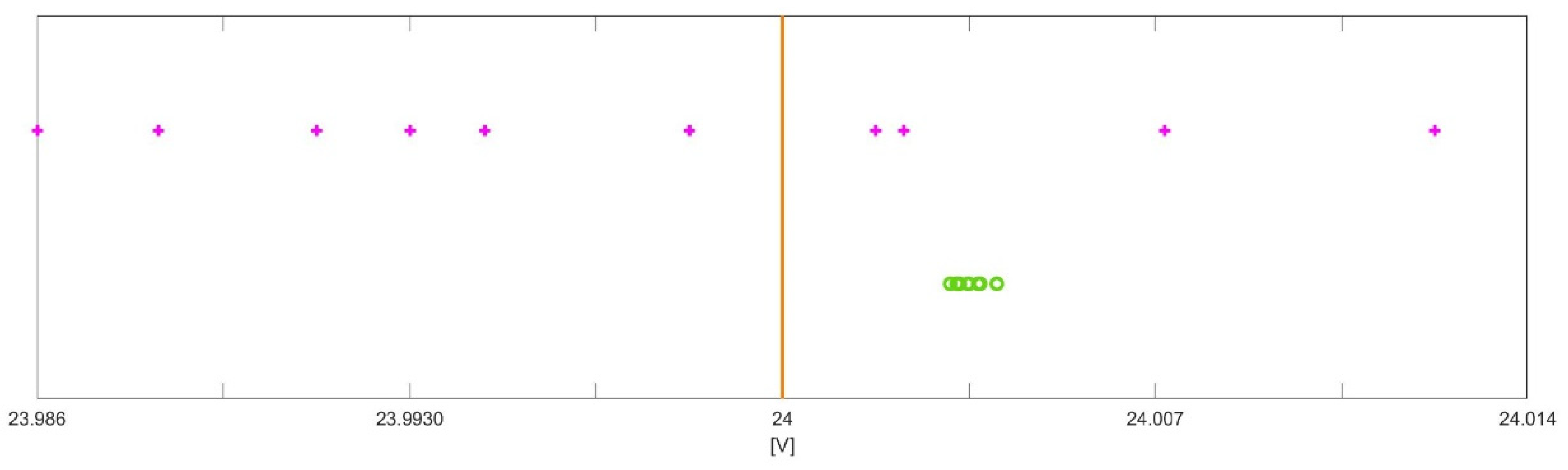
A calibrator provides a reference voltage of 24 V, and some multimeters of the same typology (4 ½ Leader 856) are employed to measure this voltage. The instrument data sheet provides the measuring accuracy as ± % of reading ± number of digits, and the value of each digit is given by the resolution in the considered range. According to the data sheet,

Table 7. The multimeter data sheet.

Multimeter 4 ½ LEADER 856
Range	Full Scale	Resolution	Measuring Accuracy
300 mV	29,999 mV	0.01 mV	$\pm \left(0.03\%Vx+0.02 \mathrm{mV}\right)$
3 V	29,999 V	0.1 mV	$\pm \left(0.05\%Vx+0.2 \mathrm{mV}\right)$
30 V	29,999 V	1 mV	$\pm \left(0.05\%Vx+2 \mathrm{mV}\right)$
300 V	29,999 V	10 mV	$\pm \left(0.05\%Vx+20 \mathrm{mV}\right)$
1000 V	10,000 V	0.1 V	$\pm \left(0.05\%Vx+0.2 \mathrm{V}\right)$

provides the resolution and the measuring accuracy in the different ranges. For the measurand $V_x=24$ V, which is the reference voltage in the proposed example, the range is 30 V and therefore, according to the specifications, the measurement accuracy is $\pm \left(0.05\%Vx+2 \mathrm{mV}\right)=\pm 0.014$ V.

Two different measurement procedures are considered:

• All multimeters are employed to measure the reference voltage.
• Only one multimeter is employed to measure the reference voltage.

Figure 2 shows, with the orange line the reference voltage and with the pink crosses the value measured by 10 different multimeters. Since different instruments are employed, it is likely to happen that the measured values fall around the reference value. In this situation, it could be possible to apply a probabilistic approach by considering the following: the mean of the measured values; an uncertainty interval around the evaluated mean, and a pdf over this interval (but only if a high number of different instruments are employed).

This situation represents very well the calibration procedure that is performed by the instruments’ manufacturer to provide the accuracy interval, which reflects the behavior of all instruments of the same typology. However, this situation is very seldom met in practice, because generally only one instrument is available and employed. Under this more common situation, when only one multimeter is employed, the value measured by the multimeter will be shifted with respect to the reference value. Moreover, if different measurements were taken, this would not help to better estimate the reference value since all measured values would be shifted more or less the same amount with respect to the reference value, as shown by the green circles in Figure 2. In fact, all measured values are taken, in this case, by the same instrument and, therefore, are affected by the same systematic error, even if a small variation can be observed, due to the presence of also random phenomena.

In this last case, even if the mean of the measured values is taken, no better estimate of the measurand can be obtained. Additionally, even if an interval is built, according to the dispersion of the measured values, this interval would not contain the value of the measurand. Therefore, to provide a good uncertainty interval, it is necessary to refer to the accuracy interval provided by the data sheet. The data sheet does not provide any pdf associated with this interval, and therefore, no pdf can be assigned to the obtained interval.

When we have a pdf over a given support, it is possible to assign a confidence interval (or degree of belief) to any subintervals of the support. However, when no pdf is assigned and no knowledge is available to assign a specific pdf, it is not possible to associate any confidence interval (or degree of belief) to any subintervals of the support. We are, therefore, perfectly in the case of Shafer’s total ignorance, where a degree of belief can be assigned to the support (or universal set), but no degree of belief can be assigned to the subintervals (to the subsets of the universal set).

It clearly follows that total ignorance is present in the measurement field. Since belief functions better represent total ignorance, it is worth exploring these functions and the theory of evidence to find an alternative, more general way to handle measurement uncertainty and measurement results. It is not the aim of this paper to provide all definitions and mathematical details, for which the readers are referred to the published literature [10,11,12,13,14]. The next section will, therefore, give only some introduction to come to the possibility distributions (PD) and the random-fuzzy variables (RFV).

5. The Random-Fuzzy Variables

In the previous sections, belief functions are introduced and it is shown how they can suitably represent the available knowledge, including total ignorance. It is interesting to observe that belief functions are a generalization of the probability functions and the necessity functions. In this respect, it is first necessary to know what a focal element is.

Let us first define the basic probability assignment function:

$$\begin{array}{c}m:P\left(X\right)\to \left[0,1\right]\\ m(\varnothing )=0\\ {\displaystyle {\displaystyle \sum }_{A\in P\left(X\right)}}m\left(A\right)=1\end{array}$$

(3)

where $X$ is the universal set, $P\left(X\right)$ is the power set of $X$ and $\varnothing$ is the empty set. According to (3), $m\left(A\right)$ represents the degree of belief that an element $x$ belongs to set $A$ (only to set $A$ and not to its subsets).

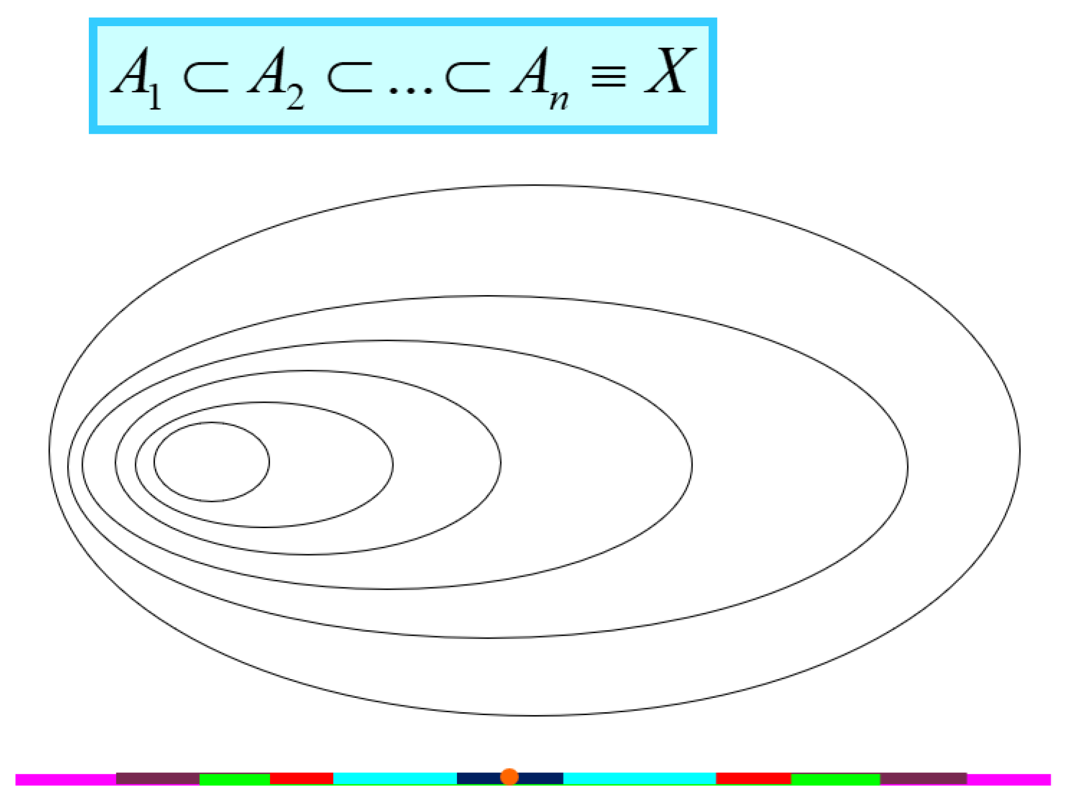
Set $A$ for which $m\left(A\right)>0$ is called the focal elements of $X$. When the focal elements are singletons, then it can be proved [9,10,11,12] that belief functions are probability functions, and the theory of evidence enters in the particular case of the probability theory. This shows that the belief functions are, as wanted by Shafer, a generalization of the probability functions. However, it is also interesting to consider another particular case of belief functions, which are called necessity functions and are obtained when the focal elements are all nested, as shown in Figure 3.

The upper plot in Figure 3 clearly shows that, when sets are considered, all sets can be ordered in such a way that $A_1\subset A_2\subset \dots \subset A_n\equiv X$. When, instead of sets, intervals are considered, the lower plot can be drawn, which still satisfies $A_1\subset A_2\subset \dots \subset A_n\equiv X$. This case is very interesting from the metrological point of view because there could be an analogy between these nested intervals and the confidence intervals of a given pdf at different, increasing levels of confidence.

The necessity function is defined as follows:

$$Nec \left(A_j\right)={{\displaystyle \sum }}_{k=1}^{j}m\left(A_k\right)$$

and represents the degree of belief that an element $x$ belongs to set $A$ and to all its subsets. When the belief functions are necessity functions, then the theory of evidence enters the particular case of the possibility theory.

In the same way that probability density functions are defined in probability, possibility distribution functions (PD) are defined in possibility as follows:

$$r:X\to \left[0,1\right]$$

where:

$$\max \left(r\left(x\right)\right)=1$$

when $x\in X$.

It can be proved [10,11] that the nested intervals of Figure 3, together with their corresponding necessity functions $Nec\left(A_j\right)$, represent confidence intervals at specific levels of confidence, coverage probability, or degree of belief $Nec\left(A_j\right)$. Therefore, remembering the GUM words that “the ideal method for evaluating and expressing measurement uncertainty should be capable of readily providing such an interval, in particular, one with a coverage probability or level of confidence that corresponds in a realistic way to that required” [1], it can be stated that the possibility theory, which provides all confidence intervals at all confidence levels, is perfectly GUM compliant.

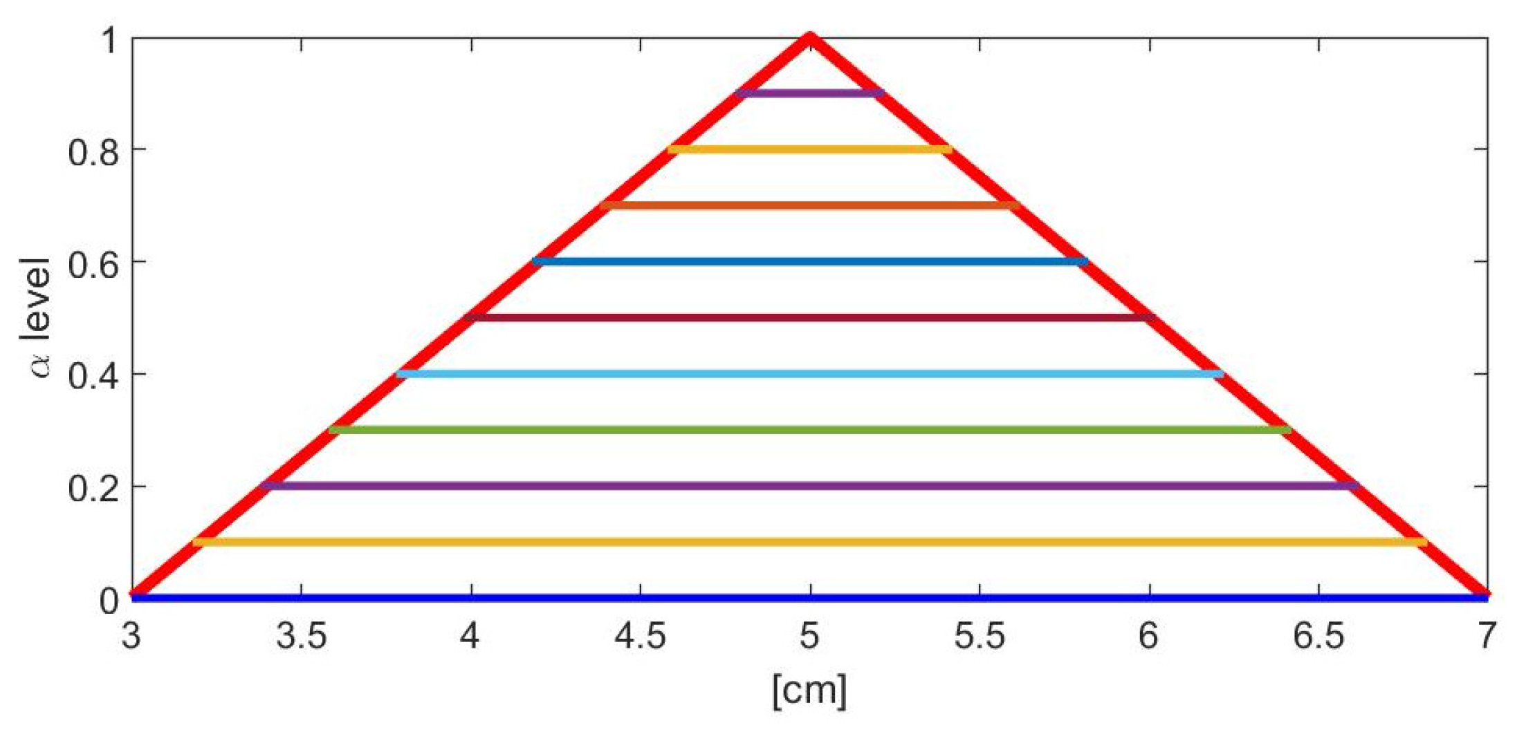
If the intervals of Figure 3 are not overlapped with each other but are positioned at different vertical levels α, such as ${\alpha }_j=1-Nec\left(A_j\right)$, then a fuzzy variable is obtained, as in the example in Figure 4.

The fuzzy variable is commonly defined by its membership function which is, from the strict mathematical point of view, a PD.

Since a fuzzy variable (a PD) represents confidence intervals at all levels of confidence, a fuzzy variable can be used to represent in a very immediate way the result of a measurement [10,11,12]. Moreover, since different kinds of uncertainty contributions may affect the measurement procedure, the best way to represent the result of a measurement is the use of a fuzzy variable of type 2 and, in particular, a random-fuzzy variable (RFV). An RFV provides two PDs and can, hence, represent separately the effects on the measurement result of the different contributions to uncertainty. An example of RFV is given in Figure 5, with the red and violet lines. In an RFV, the uncompensated systematic contributions are represented by the internal PD $r_{int}\left(x\right)$ (violet line), while the random contributions are represented by the random PD $r_{ran}\left(x\right)$ (green line). The external PD $r_{ext}\left(x\right)$ (red line) is obtained by the combination of the two PDs $r_{int}\left(x\right)$ and $r_{ran}\left(x\right)$ [10,11,12,13].

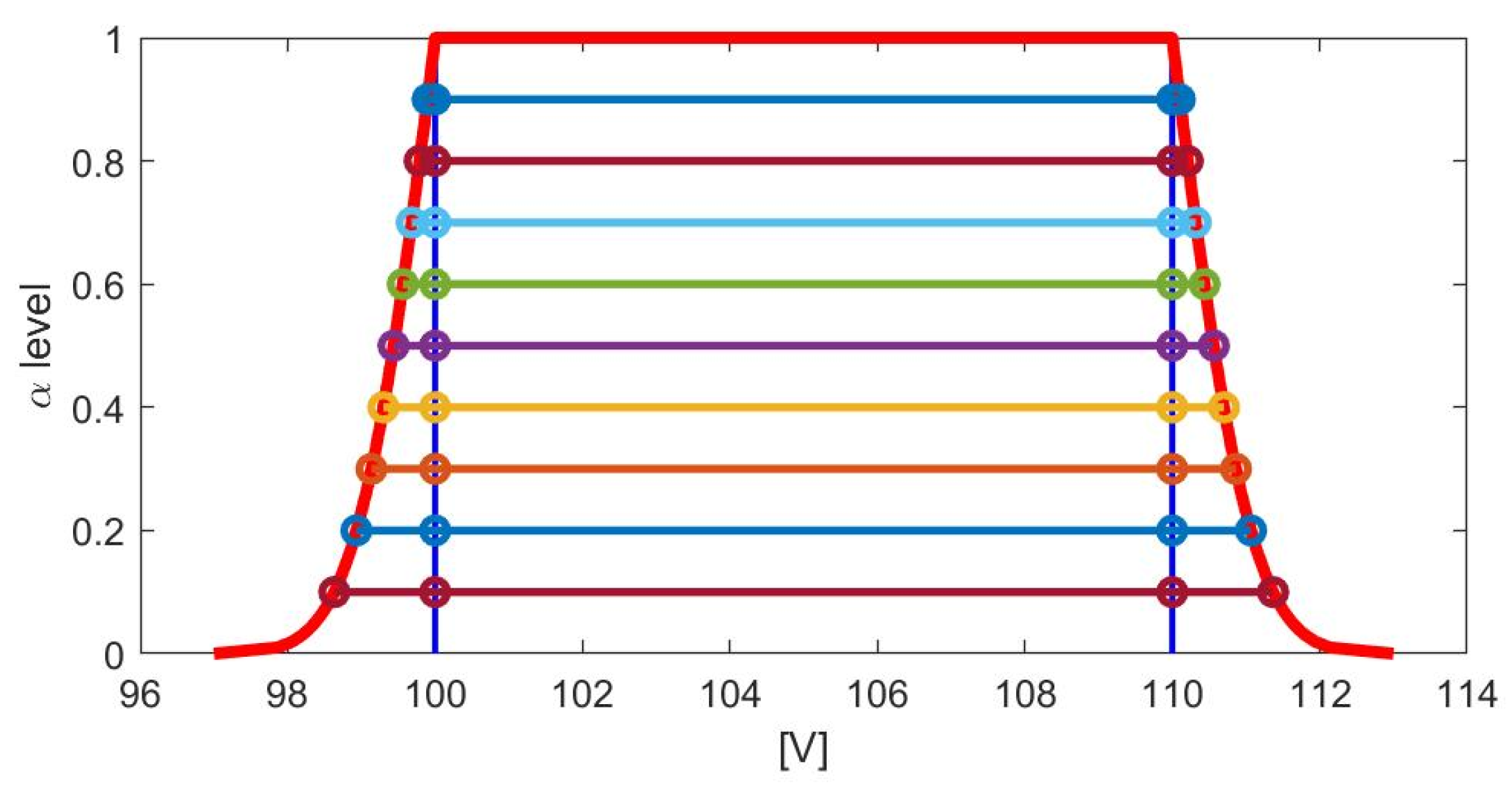
Extending the considerations made for the fuzzy variables, it can be stated that the cuts $X_{\alpha }$ at levels α of the RFV are the confidence intervals associated to the measurement result at the confidence levels $Nec\left(X_{\alpha }\right)=1-\alpha$ (as shown in Figure 6). In particular, the internal interval of each confidence interval is due to the effect on the measured value of the systematic contributions to uncertainty, while the external intervals are due to the effect of the random contributions.

If RFVs can suitably represent measurement results, then it is important to understand how an RFV can be built and how two RFVs can be combined with each other, as will be briefly explained below; we refer the readers to the literature for more details [10,11,12,13,14].

5.1. RFV Construction

To build an RFV, it is necessary to define the shape of the PDs $r_{int}\left(x\right)$ and $r_{ran}\left(x\right)$, whose construction is different [10,11,12,13,14] since they represent different kinds of contributions.

As far as $r_{int}\left(x\right)$ is concerned, this PD represents the uncompensated systematic contributions to uncertainty. As shown in the example of the multimeter in the previous Section 4, generally, the only available knowledge is, in this case, the accuracy interval given by the manufacturer of the employed instrument in the data sheet. Therefore, the available knowledge can be represented by Shafer’s total ignorance. As is also shown in Section 3, total ignorance is mathematically represented by the belief function [9,10,11]:

$$Bel\left(X\right)=1$$

$$\begin{array}{cc}Bel\left(A\right)=0& \forall A\subset X\end{array}$$

and by the rectangular PD, such as the one in violet line in Figure 5. It follows that $r_{int}\left(x\right)$ is rectangular in most situations, even if situations may exist that could lead to different shapes [10,11,12,13,14].

On the other hand, $r_{ran}\left(x\right)$ must represent the random contributions to uncertainty and therefore, in most cases, a pdf is known or can be supposed. In this case, the corresponding PD can be easily obtained by applying the suitable probability–possibility transformation (different probability–possibility transformations are available in the literature to transform pdfs into PDs. The suitable transformation when PDs are used to represent measurement results is the maximally specific probability–possibility transformation, which preserves all confidence intervals and corresponding confidence levels) [10,15].

As an example, when the pdf is uniform, then the corresponding PD is triangular; when the pdf is triangular, then the corresponding PD is the orange one in Figure 7; when the pdf is Gaussian, then the corresponding PD is the blue one in Figure 7.

5.2. RFV Combination

When the measurement results are represented by RFVs and they must be combined, it is possible to take into account all the available metrological information about the nature of the contributions to be combined and the way these contributions combine in the specific measurement procedure. According to that, since PDs can be combined using many different mathematical operators, the most proper one can be chosen.

Without entering the details, for which the readers are referred to [10,16,17], it can be stated that the random contributions to uncertainty always compensate with each other during the combination, and therefore, an operator that simulates this typical probabilistic compensation should be chosen. On the other hand, the systematic contributions to uncertainty could compensate or not with each other during the combination, according to the specific contributions and the specific measurement procedure. Therefore, there should be the possibility to choose between a mathematical operator that simulates compensation and another one which does not compensate.

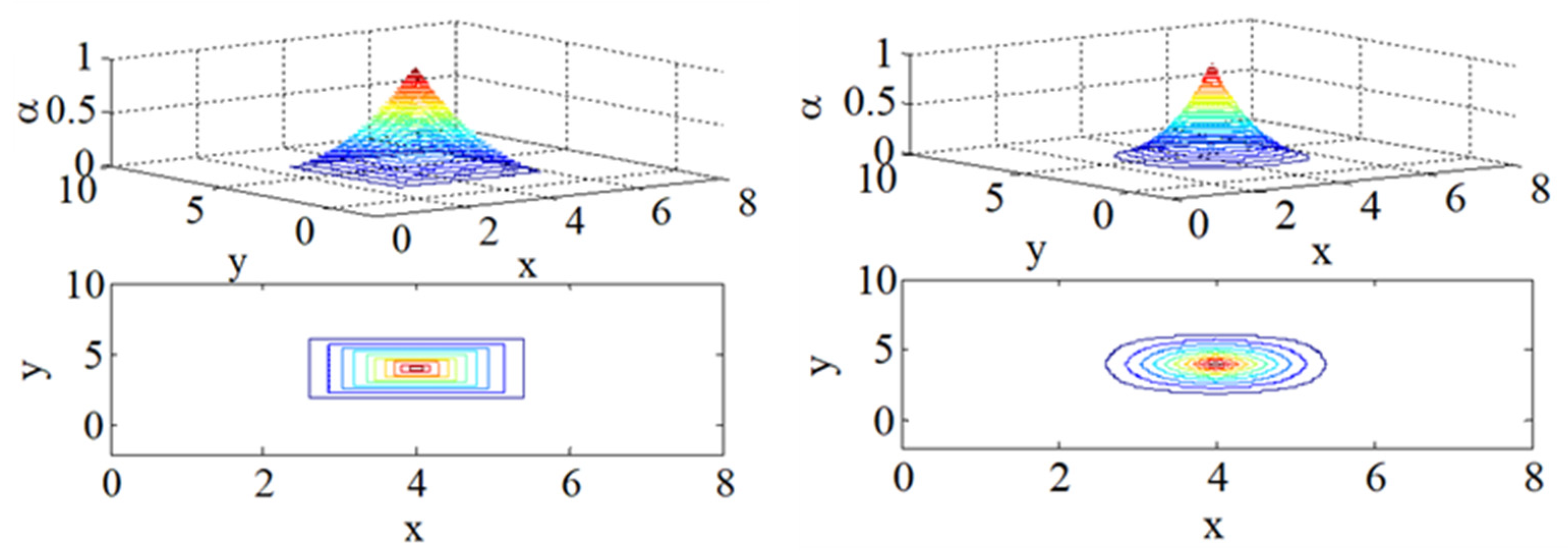
Let us first consider the evaluation of the joint PD, starting from two PDs. As an example, Figure 8 shows the results obtained by combining the same two PDs with the use of two different t-norms (for the definition of the mathematical t-norms, the readers are addressed to [15]): the min t-norm (on the left) and the Frank t-norm (on the right). In the upper plots, the two-dimensional joint PDs are shown, while in the lower plots, the corresponding α-cuts are shown. It can be easily seen how compensation applies when the Frank t-norm is employed, while no compensation applies when the min t-norm is employed.

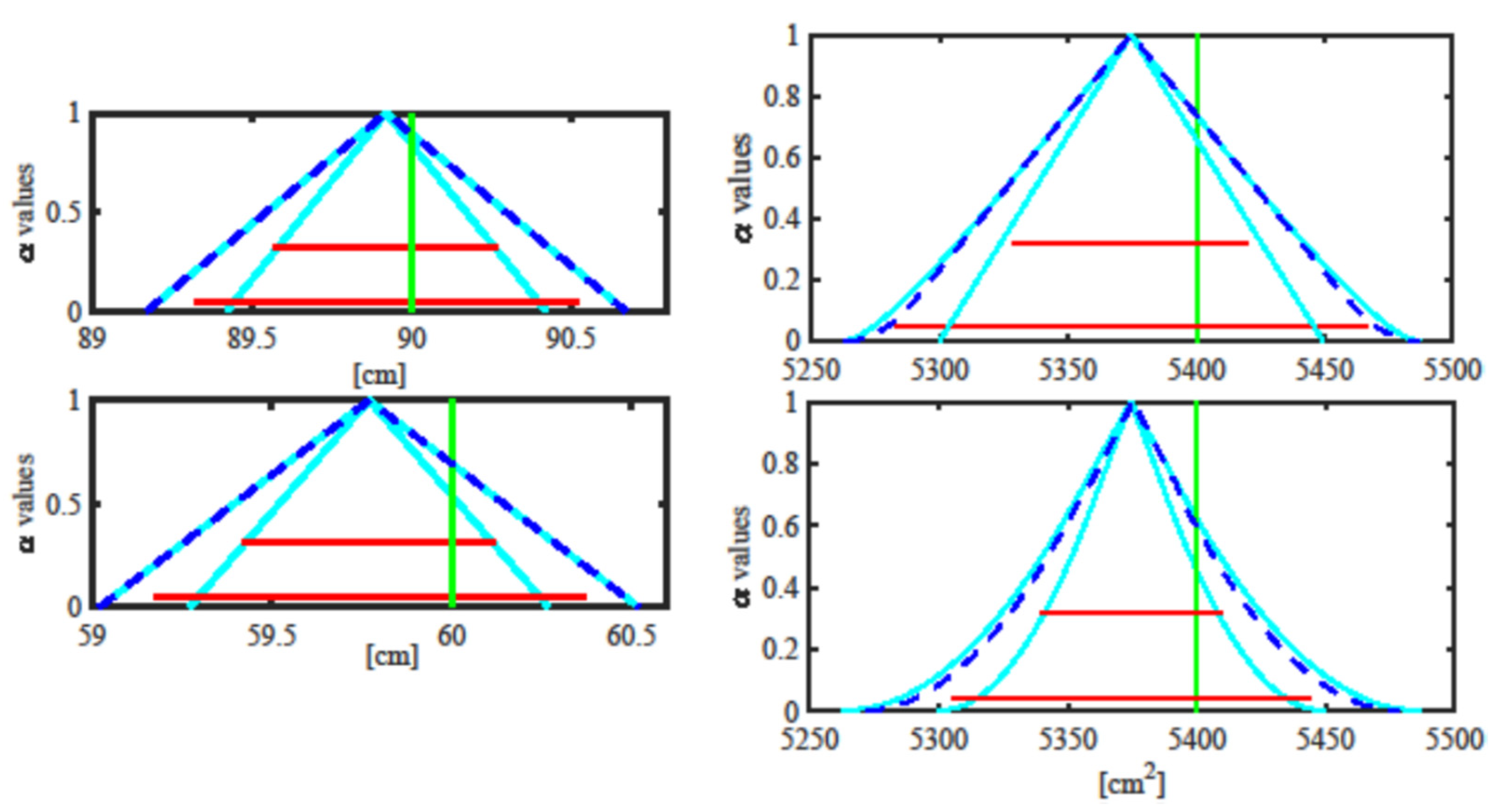
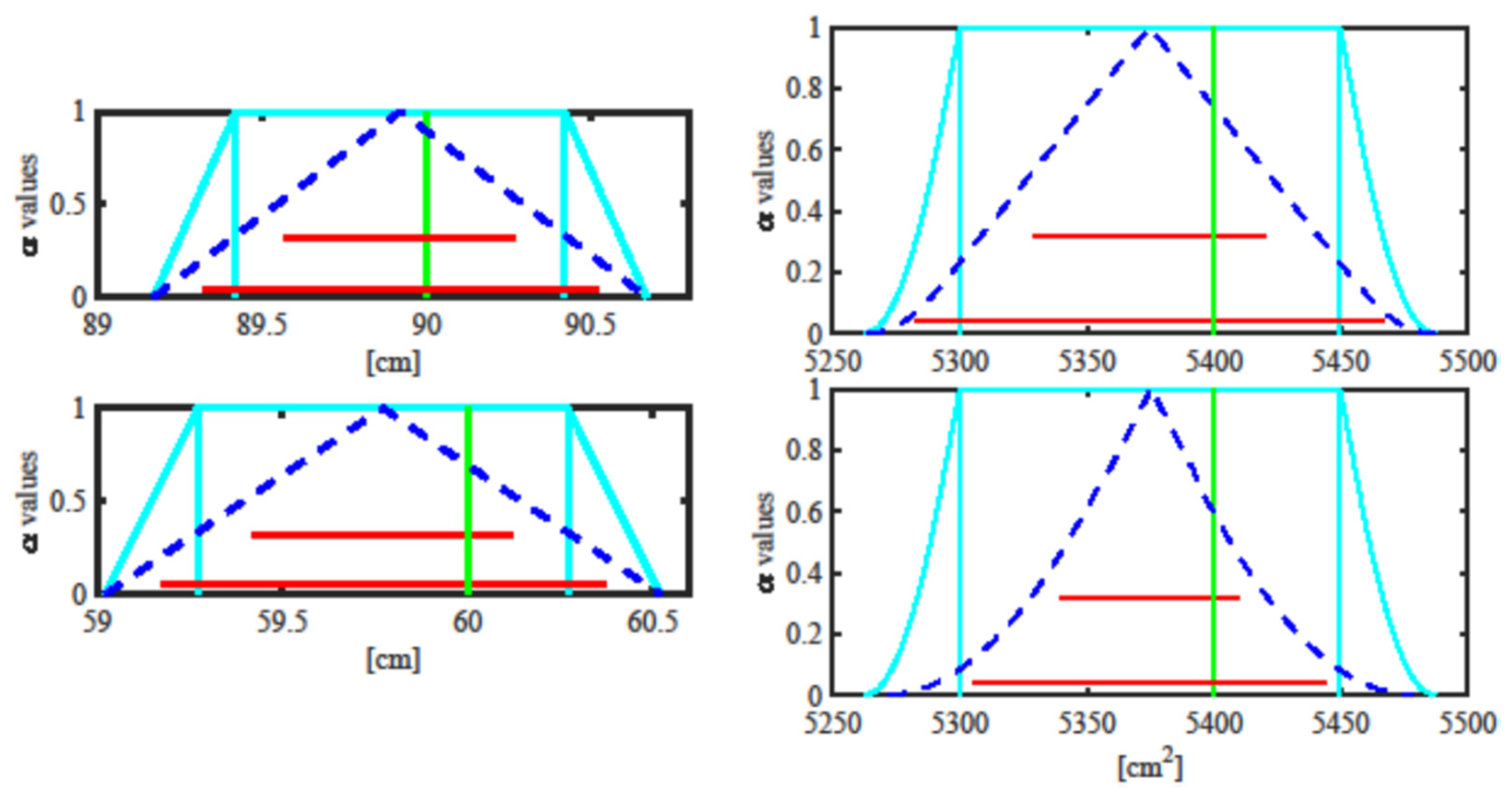
Figure 8 refers to the combination of uncorrelated contribution. Without entering the details, the correlation can also be considered, as shown, as an example, in Figure 9 and Figure 10.

From Figure 9 and Figure 10, it can be easily seen how correlation modifies the joint PDs and the corresponding α-cuts.

Once the joint PDs $r_{ran}\left(x,y\right)$ and $r_{int}\left(x,y\right)$ are obtained, it is possible to evaluate the joint PD $r_{ext}\left(x,y\right)$ and the final RFV (this is obtained by applying the famous Zadeh extension principle. The readers are referred to [9,10] for the details) [9,10,16,17].

6. Example

To show the potentiality of the RFV approach, a simple example is here reported, where the RFV approach is compared with the GUM approach [1] and the Monte Carlo approach, as suggested by [18].

The GUM approach consists of the application of the law of propagation of the uncertainty [1], while random and systematic contributions to uncertainty are combined applying the quadratic law. The results given by the GUM approach are provided in terms of two specific confidence intervals: the ones at coverage probabilities 95.45% and 68.27%. These intervals are compared with the corresponding α-cuts at the same level of confidence of the RFVs obtained with the RFV approach.

The Monte Carlo approach consists of taking extractions from the given pdfs (in a way to agree with the available information) and combining the extractions to obtain a final histogram. Then, the histogram is converted in a pdf, and the pdf is converted to a PD (through the probability–possibility transformation mentioned above) for an immediate comparison with the RFVs given by the RFV approach.

Let us come to the example. A teacher measures the length and width of her desk with a wooden ruler and evaluates the area of the desk. She/he also asks her/his pupils to take the same measurements (and the area evaluation) with measuring tapes that they have built with some white cloth and a pencil to mark the cloth every half centimeter. The measurements are taken under different assumptions about both the measurement procedure and the uncertainty contributions, as shown in

Table 8. The considered case studies.

Case	Procedure	Random	Systematic
A	Known measuring tape	uniform pdf $\pm 0.25 \mathrm{cm}$	Compensated
B	1 unknown measuring tape	uniform pdf $\pm 0.25\mathrm{cm}$	uniform pdf $\pm 0.5 \mathrm{cm}$
C	2 unknown measuring tapes	uniform pdf $\pm 0.25 \mathrm{cm}$	uniform pdf $\pm 0.5 \mathrm{cm}$
D	1 unknown measuring tape	uniform pdf $\pm 0.25 \mathrm{cm}$	$\mathrm{Interval}\pm 0.5 \mathrm{cm}$
E	2 unknown measuring tapes	uniform pdf $\pm 0.25 \mathrm{cm}$	$\mathrm{Interval}\pm 0.5 \mathrm{cm}$

.

As far as the procedures are concerned, “Known measuring tape” means that the measuring tapes are somehow characterized, and therefore, the systematic error introduced by each of them is known; since the pupil uses their own tape, the systematic error is known and can be compensated. “1 unknown measuring tape” means that both length and width are measured with the same tape taken randomly among the tapes; the systematic error introduced by the tape is not known and it cannot be compensated but, since the same tape is used for the two measurements, the two measurements are correlated with each other. “2 unknown measuring tapes” means that length and width are measured with two different tapes taken randomly among the tapes; the systematic errors introduced by the tapes are not known and they cannot be compensated and since two different tapes are used for the two measurements, and therefore, the two measurements are uncorrelated with each other.

As far as the uncertainty contributions are concerned, the random contributions are supposed to be uniformly distributed; the systematic contributions are compensated (case A), uniformly distributed (case B and C) or without any other knowledge rather than the given interval (case D and E), as in Shafer’s total ignorance situation.

The uncertainty contributions reported in Table 8 are related to the pupils’ measuring tapes, while no uncertainty is assumed to affect the teacher’s measurements, realized with the wooden ruler, so that the teacher’s measured values are considered to be the reference values $l_{ref}=90$ cm for the length and $w_{ref}=60$ cm for the width, while $A_{ref}=5400$ cm² is the reference area.

This means that, when the Monte Carlo approach is followed, extractions from the given pdfs in Table 8 are considered; when the RFV method is applied, the given pdfs in Table 8 are transformed into the corresponding PDs by applying the probability–possibility transformation; when the GUM approach is followed, the standard uncertainties are derived from the given pdfs in Table 8, that is, since the pdfs are uniform, the standard uncertainties are equal to the semi-width of the support of the pdfs divided by a factor $\sqrt{3}$ [1,2].

Without entering the details, for which the readers are referred to [10], the obtained results are shown in the following Figure 11, Figure 12 and Figure 13. When only random contributions to uncertainty are present because the systematic ones are compensated for, the three approaches provide exactly the same results, showing the validity of the RFV method in simulating the presence of the random contributions. When both random and systematic contributions are present and their associated pdfs are known, the GUM approach underestimates the final measuring uncertainty, while the RFV and the Monte Carlo approaches provide very similar results. In this case, the RFV approach has the advantages of being faster and distinguishing, in the final measurement result, the effects due to the two different kinds of contributions. Finally, in the case of total ignorance, neither the GUM or the Monte Carlo approach can represent it in a different way with respect to cases B and C; therefore, they provide incorrect results.

7. Conclusions

This paper represents a review paper of the RFV approach, proposed in the literature in the last decades.

It has been shown the potentiality of this approach, which is able to represent and propagate measurement results in closed form, by simulating the way the uncertainty contributions propagate through the measurement procedure.

Other more specific applications are present in the more recent literature, like for instance the generalization of Bayes’ theorem in the possibility domain [19,20] or the realization of a possibilistic Kalman filter [21,22], thus showing the versatility of the RFV approach.