Article

The Role of Structural Inequality on COVID-19 Incidence Rates at the Neighborhood Scale in Urban Areas

1
Department of City & Metropolitan Planning, University of Utah, Salt Lake City, UT 84112, USA
2
Department of Atmospheric Sciences, University of Utah, Salt Lake City, UT 84112, USA
3
Division of Pulmonary and Critical Care Medicine, Department of Internal Medicine, School of Medicine, University of Utah, Salt Lake City, UT 84112, USA
4
Department of Political Science, University of Utah, Salt Lake City, UT 84112, USA
5
Department of Mining Engineering, University of Utah, Salt Lake City, UT 84109, USA
6
Department of Life, Earth, and Environmental Sciences, West Texas A&M University, Canyon, TX 79016, USA
7
Division of Epidemiology, Department of Internal Medicine, School of Medicine, University of Utah, Salt Lake City, UT 84112, USA
*
Author to whom correspondence should be addressed.
COVID 2021, 1(1), 186-202; https://doi.org/10.3390/covid1010016
Submission received: 26 June 2021 / Revised: 26 July 2021 / Accepted: 28 July 2021 / Published: 4 August 2021

Abstract

:
The lockdown policies enacted in the spring of 2020, in response to the growing severe acute respiratory syndrome coronavirus 2 (SARS-CoV-2) pandemic, have remained a contentious policy tool due to the variability of outcomes they produced for some populations. While ongoing research has illustrated the unequal impact of Coronavirus disease (COVID-19) on minority populations, research in this area has been unable to fully explain the mechanisms that produce these findings. To understand why some groups have been at greater risk of contracting COVID-19, we employ structural inequality theory to better understand how inequality may impact disease transmission in a pandemic. We used a novel approach that enabled us to focus on the microprocesses of structural inequality at the zip code level to study the impact of stay-at-home pandemic policies on COVID-19 positive case rates in an urban setting across three periods of policy implementation. We then analyzed data on traffic volume, income, race, occupation, and instances of COVID-19 positive cases for each zip code in Salt Lake County, Utah (USA) between 17 February 2020 and 12 June 2020. We found that higher income, percent white, and white-collar zip codes had a greater response to the local stay-at-home order and reduced vehicular traffic by nearly 50% during lockdown. The least affluent zip codes only showed a 15% traffic decrease and had COVID-19 rates nearly 10 times higher. At this level of granularity, income and occupation were both associated with COVID-19 outcomes across all three stages of policy implementation, while race was only predictive of outcomes after the lockdown period. Our findings illuminate underlying mechanisms of structural inequality that may have facilitated unequal COVID-19 incidence rates. This study illustrates the need for more granular analyses in policy research and adds to the literature on how structural factors such as income, race, and occupation contribute to disease transmission in a pandemic.

1. Introduction

The lockdown policies enacted in the spring of 2020, in response to the growing severe acute respiratory syndrome coronavirus 2 (SARS-CoV-2) pandemic, have remained a contentious policy tool due to the variability of outcomes they produced for some populations [1,2,3]. Many studies have been conducted to investigate the impacts of variations in socioeconomic, demographic, racial, and geographical factors in the incidence of Coronavirus disease (COVID-19). While ongoing research has illustrated the unequal impact of COVID-19 on minority populations [4,5,6,7,8,9], efforts in this area have been unable to fully explain the mechanisms that produced these findings. A clear outcome from a number of studies around the world is that racial and ethnic minority populations are experiencing a disproportionate burden of COVID-19, which is only partially explained by structural factors [10,11,12,13,14,15,16]. As research in this area relies on incomplete or suboptimal data aggregated to the county, state, and national levels, uncertainty remains as to why these patterns persist [17,18]. This study attempts to contribute to this growing body of research.
The influence of social, economic, and racial disparities on the spatial incidence and mortality of COVID-19 has received increasing attention [19,20] and the findings are stark. A national study spanning 3141 US counties found an association between racial/ethnic population, economic inequality, and COVID-19 incidence and mortality [21]. For example, an analysis of spatial determinants of COVID-19 transmission in the United States found that African American populations in urban areas had the highest COVID-19 case and death rates at the county and state level [22], even after controlling for age, sex, socio-economic status, and comorbidities [23]. Additionally, emerging research on COVID-19 suggests a link between race, socioeconomic status, and virus prevalence [24,25,26,27]. Other significant associations between COVID-19 incidence include percentage of foreign-born population, percentage of households with no vehicle, and percentage of people over 65 years old [28].
To understand why some groups have been at greater risk of contracting COVID-19, we employ structural inequality theory [29]. Structural inequality is a system of privilege created by institutions (i.e., law, government, and media) and their related norms (e.g., business practices) and policies (e.g., healthcare, education, land use, etc.) within society. Research on structured inequality often studies the processes and consequences of inequality found at the intersection of racial or ethnic minority status, class, income, gender, education, and/or occupation, among others [30,31].
According to Sørensen (1996), there are two ways structure can promote inequality: through structural effects on the individual (making them more or less productive in society) or through the advantages and disadvantages of one’s position within the social structure (giving individuals an unequal starting point) [32]. When the latter occurs, properties of the individual’s position in society helps to determine their income and other rewards, independently of the characteristics of the individual [32]. Together, these structures create relational patterns that effectively socialize and dictate how individuals see the world and their place in it. Inequality is considered structural when policies produced by the system keep some groups from getting ahead, regardless of their actions. This type of inequality is harmful to society more generally, as it is economically inefficient, produces conflict within society, and creates a less productive workforce overall [29].
To study the structural factors of inequality and how they impact disease transmission in a pandemic, we use a novel approach that enables us to focus on the microprocesses of structural inequality at the zip code level. For the greatest generalizability, this study takes place in Salt Lake County (SLCo), Utah (USA), which is a diverse urban setting with over 1.16 million inhabitants of varying income levels and a large immigrant population. Most importantly, SLCo has a state-of-the-art traffic count network, which can be used to study human behavior in a natural setting and at varying scales [33,34,35,36,37,38]. These characteristics present a unique opportunity to better understand the structural factors and unequal impacts of COVID-19 on low-income, minority, and occupation types on COVID-19 transmission at the zip code level.
Despite the value of studying communities at the subcounty level, research at this level of analysis is generally difficult to conduct as data sources of this granularity are rarely available due to cost and feasibility. Therefore, efforts to collect, study, and improve available data on social-demographic factors at a fine resolution (i.e., the zip code level) are still needed [16], but are expected to be fruitful. For instance, a recent study used negative binomial regression models to investigate the association between zip code, racial composition, and disparities in hospitalization and mortality for COVID-19, and found that each 1% increase in a black population in a zip code was associated with a 3% increase in COVID-19 cases [39]. Additionally, at the zip code level, household size, rather than population density, was found to be the largest single driver behind variations in COVID-19 rates [40]. A zip code analysis of COVID-19 incidence rates in Illinois and New York City also found that crowded households, high poverty, and racial differences yielded “stark contrasts” to households that were less crowded, lower poverty and who that were less racially diverse [41].
In addition, recent studies that attempt zip code level analysis have been foundational for advancing structural inequality theory and extending our knowledge of COVID-19 outcomes. For instance, Harris (2020) shows that wealth and ethnicity are key factors in COVID-19 mortality rates [42]. Likewise, Lan et al. (2020) illustrate the increased risk of COVID-19 infection based on occupation in selected zip codes [43]. Vahidy et al. (2020) applied a range of medical and demographic factors on COVID-19 outcomes using hospital data, but only as it applies to Hispanic populations [44]. However, research in this area largely assesses neighborhoods in terms of socioeconomic factors and resulting disparities [45,46] and at times, key factors (i.e., income or occupation) are excluded and only race is explored [47]. Since research at this level is important for confirming that the intersectionality of several factors, not race alone, best explain COVID-19 outcomes and why minorities are impacted more than white populations.
While the study of health disparities can be related to a range of compounding factors [48,49,50,51], economically disadvantaged populations often face the highest levels of health-related risk, which are confounded by structural factors such as minority status, education, and occupation [52]. As essential workers have been especially impacted by COVID-19 [53], we also consider the role of occupation in the transmission of disease. We reasoned that individuals in lower income brackets are more likely to work in sectors that are classified as essential or blue-collar and, therefore, would still be expected to work during the study period. In contrast, individuals in higher income brackets are more likely to work in occupations considered white-collar and, therefore, would have the increased ability to work from home [54]. While it is widely recognized that occupation and location jointly contribute to social stratification and inequality [55,56,57], occupation alone is considered the most strongly correlated factor of social status and life opportunity [58]. As a result, we find it appropriate to further investigate how structural factors contribute to the mechanisms of transmission risk that explain the unequal spread of COVID-19 in urban settings.
To explore this area of research, we examine the impact of one type of social distancing policy, Utah’s “Stay Safe, Stay Home” (SSSH) directive (hereafter referred to as “Lockdown”), on the cumulative incidence rate of COVID-19 positive cases (hereafter “COVID-19 cases”) in SLCo. We aim to understand how structural factors may help to explain the variation in COVID-19 incidence rates in some zip codes of SLCo over others. To understand the relationship between pandemic policies and structural factors of inequality, we compare traffic counts, as a proxy for mobility, and COVID-19 cases by zip code over three phases of policy implementation between 17 February and 12 June 2020. We also overlay these findings with data on income, race, and occupation during this same period to better understand the compounding role of demographic factors on the transmission of COVID-19.

2. Materials and Methods

Our research explores three propositions about the relationship between lockdown policies, structural factors of inequality, and COVID-19 positive case rates. First, we examine the impact of stay-at-home policies on traffic volume through three distinct periods of policy implementation to determine if such patterns were equivalent across all neighborhoods. Second, we explore if zip codes with higher rates of vulnerable populations (e.g., low-income, minority, or blue-collar workers) have equal traffic variability as populations from less vulnerable zip codes (e.g., high income, white, or white-collar communities). Third, we analyze whether traffic mobility is associated with COVID-19 cases and how such patterns overlap with income, race, and occupation data, to understand what this relationship might imply for policy and future research.

2.1. Study Timeline

Our study focused on the three phases of policy implementation for the local stay-at-home directive, which occurred during the early stages of the COVID-19 pandemic in 2020. We define each phase in the following way. The Pre-Lockdown period, from 17 February–15 March, includes the four weeks prior to the start of the Lockdown policy. The Lockdown period, from 16 March–26 April, is the lockdown phase of the policy where Utahns were asked to remain at home. The final phase or Post-Lockdown period, from 1–28 May, includes the easing period following lockdown policy. We lag the COVID-19 case count data by 14 days (until 11 June 2020) to account for the broadly accepted incubation stage of the virus.

2.2. Data Sources

SLCo is composed of 38 zip codes with a population greater than zero. Of the 38 zip codes, 34 were included in this study and 4 were excluded due to lack of data or other relevant data availability issues. More detailed information on SLCo is provided in Appendix A. Briefly speaking, COVID-19 daily case counts for the 34 remaining zip codes were obtained from the Salt Lake County Department of Health’s COVID-19 dashboard [59]. The study also uses sociodemographic data drawn from the “Healthy Salt Lake” dashboard [60], and includes variables for total count and precents by each population type, percent white population, average household size, occupational group, and median income by zip code. Traffic count data was accessed through two data portals. The traffic counts for Utah roads and highways are available through Automated Traffic System Performance Measures (ATSPM) [35], and the counts for interstate traffic are obtained from the Performance Measurement System (PeMS) [36]. This data is aggregated by zip code, and daily counts were extracted from 4 March 2020 (when COVID-19 cases were first reported in Utah) to 11 June 2020 (two weeks following the study end date to account for the viral incubation period).

2.3. Statistical Methods

Change in traffic volume and COVID-19 cumulative incidence rates was derived using medians of each category to determine the central tendency of the group. Medians were the preferred statistic for comparison due to the varied lengths of the Pre-Lockdown, Lockdown, and Post-Lockdown periods, the non-normal nature of sample data collected, and inclusion of outliers in the dataset [61]. Means are not an appropriate tool for this research, as taking a mean requires inclusion of those outliers, which could distort the findings and provide false insights. Accordingly, median based, non-parametric methods were used for data analysis for robustness. A Kruskal–Wallis rank sum test was performed to quantify the difference in traffic volume and COVID-19 positive case rate change across the structural factors and study periods: Pre-Lockdown to Lockdown, and Lockdown to Post-Lockdown. We then used Dunn’s test, with the Bonferroni Correction, to identify statistically significant pairs associated with each structural factor, and to adjust p-values from running the risk of Type-I error in case of multiple statistical tests [62]. For both tests, the null hypothesis would result in no statistically significant differences across groups. Data processing and analysis was performed using Matlab Version R2019b [63] and R Version 3.6.3 software [64].

3. Results

Based on our analysis, the three main propositions we explore present a highly nuanced view of the impact of lockdown policies at the neighborhood level. With this granularity, several important patterns emerge that shed light on the unequal benefit the policy produced. Specific factors of importance include (1) the impact of data aggregation at the county, state, or regional levels on study outcomes; (2) disjunctions between human mobility (voluntary or otherwise); (3) structural factors of inequality (e.g., income, race, and occupation); and (4) the spread of disease. The following section reviews each research question in detail.

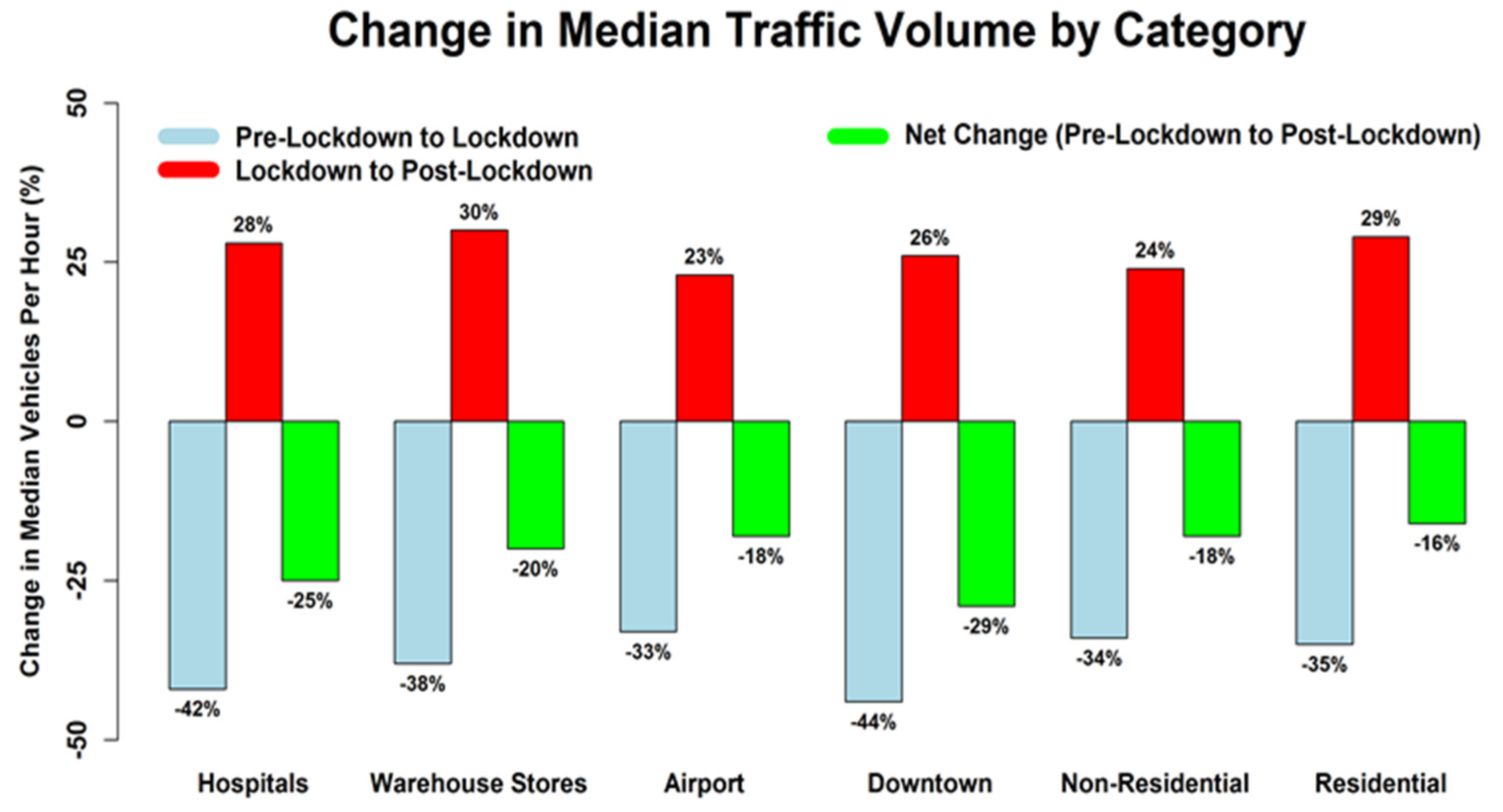
3.1. Proposition 1: Do Social Distancing Policies Keep People at Home (or Impact Mobility) as Intended?

Our first proposition studies the impact of the lockdown policy on COVID-19 outcomes over the three periods of policy implementation. Figure 1 shows that the traffic volume in SLCo decreased by 30–40% with the onset of the lockdown policy and rebounded by 20–30% as these policies were slowly relaxed in the Post-Lockdown period. When all major categories of the built environment are compared, they produce similar outcomes across the study periods.
When we move from the aggregate level to the zip code level, however, a much more disparate pattern emerges. At this level, we find that the Pre-Lockdown median volume of residential weekday traffic ranged from 54 to 1816 vehicles per hour (vph), as shown in Appendix A, Table A1. In stage two of the implementation period, when the county was under the lockdown directive, the median ranged from 42 to 1191 vph. In the Post-Lockdown period, the median traffic volume ranged from 53 to 1487 vph. As the pandemic was ongoing, it is unsurprising that the rebound remained below the initial vph values. However, the variability found in the second and third period of policy implementation suggests that lockdown directives may have had limited impact in some zip codes in relation to others.

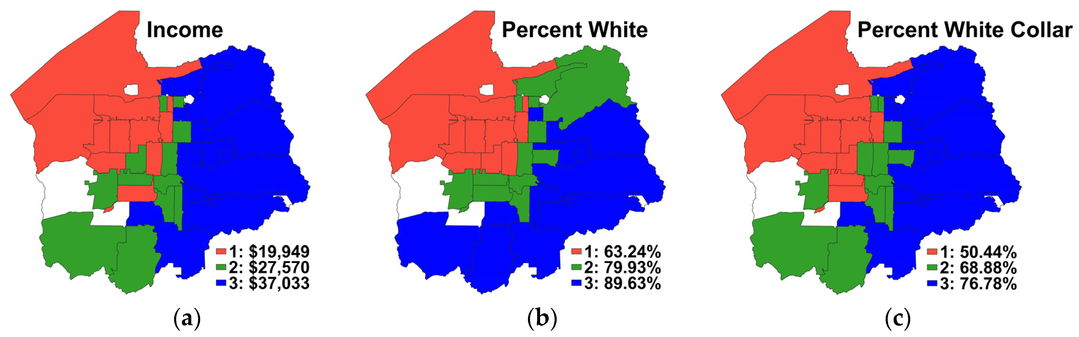
3.2. Proposition 2: Do Stay-at-Home Orders Benefit All Populations Equally?

Table 1 shows the relationship between changes in human activity that resulted from the lockdown policy with traffic volumes grouped by structural factor (e.g., income, race, and occupation) and ranging in groups from lowest (Group 1) to highest (Group 3).
Table 1 also shows the relationship between changes in human mobility when the categories are grouped by the percent of white population (with lowest groups being the least white). Table A2, found in the Appendix A, is analogous to Table 1, but uses means instead of medians, with similar results. In the transition from the Lockdown to Post-Lockdown period, Table 1 shows that the lowest income group has the lowest bounce back in traffic (18%), while the highest income group has a markedly higher bounce back in traffic with levels of more than double (36%) that of other groups. When traffic and race are compared by zip code in the Pre-Lockdown period, the volume of traffic was comparable across all groups with the middle group starting with slightly more traffic than the others. When race is analyzed in the transition from Pre-Lockdown to Lockdown policy periods, we found the reduction in traffic volumes followed a similar pattern as income; however, the middle group showed the largest decrease. In a similar manner as the income analysis, Group 3 (most white) had the largest increase in traffic following the shutdown, with Group 1 showing less than half the increase.
Finally, Table 1 also shows the relationship between changes in human mobility and categories that are grouped by percent of white-collar occupation (with highest groups being the most white-collar). In the Pre-Lockdown stage, baseline traffic volumes are nearly identical as when grouped by income. This seems to confirm the notion that income and occupation are closely related. Similarly, the variation in traffic from Pre-Lockdown to Lockdown to Post-Lockdown period shows similar patterns to the income analysis. Based on these findings, our analysis seems to suggest that lower income, minority status groups, and least white-collar workers have not equally benefitted from the lockdown policy either during and/or following the lockdown period.
Table 2 illustrates the results of the Kruskal–Wallis rank sum test. Here, our null hypothesis states that the traffic change was not statistically significant across structural factors. Table 2 shows that one structural factor and time period combination was statistically significant at the p ≤ 0.001 level, two were statistically significantly different at the p ≤ 0.01 level, and three were statistically significant at the p ≤ 0.05 level.
The pairwise comparisons of percent median traffic change among sociodemographic groups for the different study time periods using Dunn’s test are shown in Table 3. There are four statistically significant results at the p ≤ 0.05 level: one each for the income and percent white variables, and two for the percent white collar variable. Two of the statistically significant results occurred from the Pre-Lockdown to Lockdown periods, and two occurred from the Lockdown to Post-Lockdown periods. Additionally, there are two statistically significant results at the p ≤ 0.01 level, which includes one for the percent white variable in the Lockdown to Post-Lockdown period and the other for the percent white-collar variable in the Pre-Lockdown to Lockdown period. Lastly, there is one statistically significant result at the p ≤ 0.001 level for the percent white variable in the Lockdown to Post-Lockdown period.
Based on this analysis, we find that when traffic and income levels are compared by zip code in the Pre-Lockdown policy implementation stage, the volume of traffic was comparable in all three groups, but the highest income group (Group 3) notably began with less traffic than the others. In the transition to the lockdown period, we found the reduction in traffic to be lowest in Group 1 (−29%) and highest in Group 3 (−40%). These differences were found to be statistically significant and are shown in Table 3. Likewise, in the transition from the Lockdown to Post-Lockdown period, the lowest income group shows the lowest bounce back in traffic, while the highest income group has a markedly higher bounce back in traffic with levels of more than double that of other groups. Thus, the reduction in traffic from Pre-Lockdown to Lockdown to Post-Lockdown periods are closely patterned on income with higher income groups, reducing mobility in response to the lockdown policy and lower income groups, less so. As illustrated in Table 3, we found statistically significant differences between Group 1 and 3, and Group 1 and 2 for white collar populations.

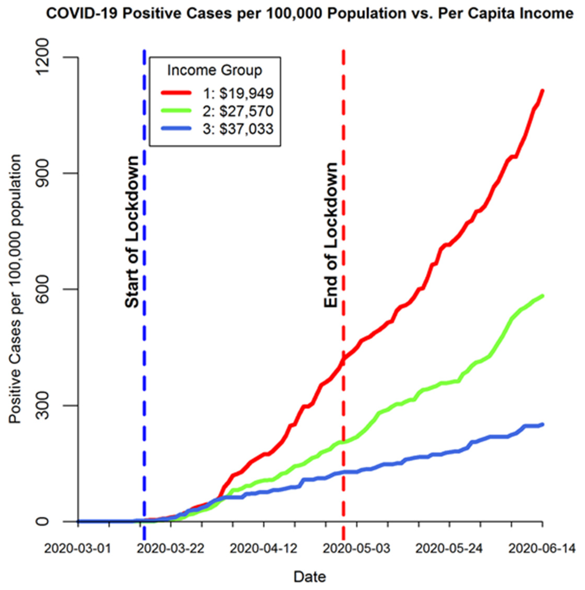
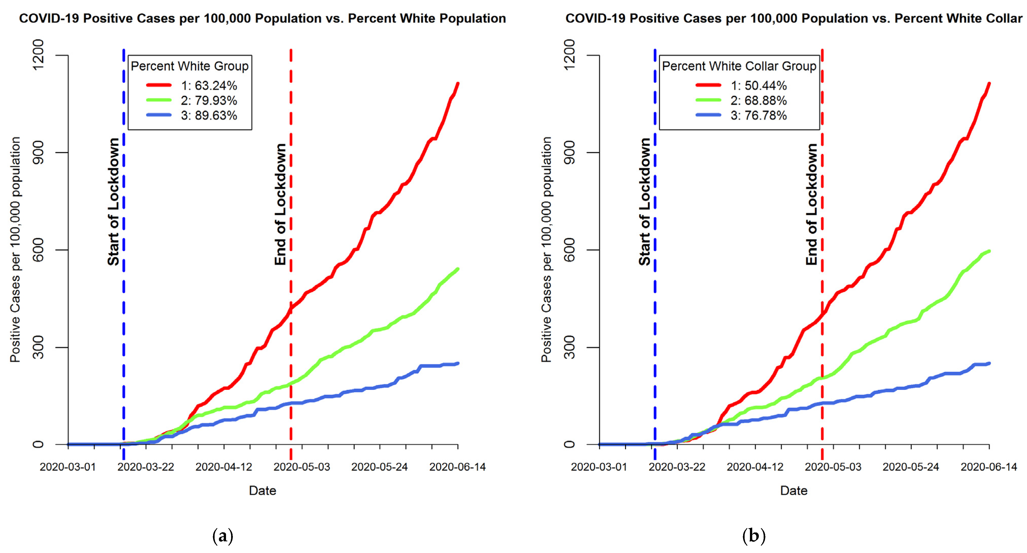
3.3. Proposition 3: Do All Groups Have Similar COVID-19 Incidence Rates?

As an association has been demonstrated between income level, race, occupation, and traffic patterns following the three policy periods of this study, we then compared these factors with COVID-19 cases by zip code (Figure 2 and Appendix A, Figure A1). The analyses and figures refer to cumulative positive case counts.
For this proposition, the null hypothesis is that there is no difference in the change of positive COVID-19 case rates across structural factors. We found all three structural factors were statistically significantly associated with the COVID-19 case count changes from the Pre-Lockdown to Lockdown period, but not those from the Lockdown to Post-Lockdown period (Table 4).
The pairwise comparisons of COVID-19 positive case change among structural factors for the different study time periods using Dunn’s test are shown in Table 5. There is one statistically significant result at the p ≤ 0.05 level, three at the p ≤ 0.01 level, and one at the p ≤ 0.001 level. One of these statistically significant results belongs to the percent white-collar variable, and two each belong to the income and percent white variables. As in Table 4, the statistically significant results are only present when comparing the Pre-Lockdown to Lockdown periods. All comparisons between zip codes belonging to the most vulnerable populations (Group 1) to the least challenged (Group 3) are statistically significant.
As shown in Figure 2 and Appendix A, Figure A1, based on this analysis, we find that, overwhelmingly, lower income, minority populations, and least percent white-collar zip codes had higher COVID-19 cases. The lowest income zip code (84104) of Salt Lake County had the lowest percent white population (50.13%) and the highest rate of COVID-19 positive cases (1214.64 positive cases per 100,000). In contrast, the highest income zip code (84108: USD 43,068) had the thirteenth highest percent white population (85.77%) and second lowest rate (138.19 positive cases per 100,000). Additionally, lower income (Figure 2), lower percent white (Appendix A, Figure A1a), and lower percent white-collar (Appendix A, Figure A1b) zip codes show greater growth in positive COVID-19 case rates throughout all policy phases. The difference in COVID-19 case growth is most clearly visible in the Pre-Lockdown to Lockdown period for all structural factors (Table 5).
It is important to note that, the clear difference in COVID-19 incidence rates between Groups 1 and 3 notwithstanding, the incidence rate was high for all groups. Therefore, one could reasonably conclude that though the lockdown policy helped bring down incidence rates, it did not do as adequately as policy makers and scientists alike had hoped. However, as COVID-19 incidence rates were higher after the Lockdown period, it is likely that the rates could have been markedly higher had lockdown policies not been implemented.
Furthermore, when these same demographic factors are laid out geographically on COVID-19 positive case rates by zip code, as illustrated in Figure 3, income and percent white-collar rates of COVID-19 are almost identical. As noted by the red color, the most socioeconomically challenged groups are basically invariant across all three factors when grouped by zip code. In contrast, the middle and least challenged groups (green and blue) show some variability across the same factors, while always remaining in a more affluent category than the first group.
These findings seem to suggest that high percent minority populations are a good indicator of least white-collar and lower income jobs in this urban area, while the inverse is not necessarily true. This reflects the fact that the SLCo area has a majority white population that spans a wide range of income levels and occupations, making this case especially interesting, as it demonstrates the compounding impact of socioeconomic status regardless of race. As Utah has some of the largest household sizes in the United States, the overall per capita income is much lower than presented here, which implies that our findings are likely further understated in the less affluent categories.
Likewise, while SLCo offered free and plentiful testing from the onset of the pandemic, due to concerns over selection bias in our sample resulting from intentionally suppressed testing, under testing, and unequal access to testing for reasons outside of availability [65], we tracked positivity rates by zip code over the study period. Based on these efforts, we found that positivity rates (e.g., percent positive cases/total tests) were consistently higher for less affluent communities, as expected. For example, over the study period, the lowest income neighborhood (84104: USD 14,533) has a positive rate of about 21%, while the most affluent neighborhood in our sample (84108: USD 43,068) has a positivity rate of only 13% [59]. This suggests that the findings presented here may be understated when compared at the zip code level.

4. Discussion

While emerging research suggests that pandemic policies have not resulted in equal outcomes for all populations, this research illustrates how improvements in data quality and granularity have been fruitful for advancing understanding in this area. For instance, we found that zip code level analysis of the impact of the lockdown policy on disease outcomes was effective at strengthening the discussion from previous research by illustrating the microprocesses at play in the spread of COVID-19. Similar to previous studies, we found that some zip codes responded to the stay-at-home directive at a greater magnitude than others, and this change persisted across all three policy periods. However, at the zip code level, we were able to show that income and occupation, not race, were the greatest factors of interest in this case. Thus, structural factors in tandem are more likely the cause of variability in COVID-19 outcomes. Furthermore, we found the zip code level analysis was critical in exposing these patterns. When aggregated, these findings seem to have been obscured, and critical policy impacts might otherwise go unidentified, thus further harming unfairly affected groups within society.
Considering prior works, our focus on COVID-19 outcomes by income, race, and occupation, revealed an even starker pattern. For example, based on this analysis, we can conclude that the lockdown policy had a greater benefit on higher income, white population, and white-collar workers throughout the policy periods. Here, race was not a strong determinate of outcomes. However, upon easing of the policy, higher income, low minority status communities showed a rapid resurgence to activity, while lower income, high minority status communities, which had not seen a decline in activity across the policy implementation stage, showed a smaller rebound in activity. We attribute this to the ability of affluent communities to shelter at home, avoid the harms of COVID-19 (physically, mentally, and economically), and then return to their normal activities following the lockdown period. This is a much more nuanced pattern than has been previously presented in the literature.

4.1. Implications

The most important finding of this research is the clear, but complex relationship between traffic volume, race, income, occupation, and COVID-19 outcomes at this level of granularity. The increased variability found in the second and third period of policy implementation suggests that lockdown directives may have had limited impacts on the most vulnerable groups. Thus, we add to the literature on structural factors of inequality, and specifically how these factors interact with public health, public policy, and disease transmission. Such findings help explain the underlying mechanisms that produced unequal COVID-19 incidence rates. It may also help inform future policy solutions, as stay-at-home and lockdown policies will need to be redesigned to address the variability in effectiveness and to prevent additional harm if they are to be used again going forward.

4.2. Limitations

Some limitations in the data and methodology warrant mention. This paper reports on the impacts of COVID policies on some aspects of society. However, determining the causes of COVID incidence rates was out of the scope of this research. The associations found in this study suggest a number of relationships, but definitive causal relationships are not attempted. As a result, we only present key findings of strong significance in the observed changes at certain COVID-19 incidence rate inflection points, which are very important in terms of structural inequality. In addition, issues with data availability and quality may also cause limitations for this research. COVID-19 cases may be under-reported or geographically biased due to differing testing rates. Additionally, a disproportionate number of deaths from CoV-SARS-2 occurred in long-term care facilities and other clustered communities, which may be more consequential in future studies. However, as income, race, and occupation share some similar patterns, and sometimes mirror the incidence of disease, it seems less likely that these variables impact internal validity in a similar manner to produce these outcomes. This may also reflect the very real issue of structural inequality, a concept that has been difficult to trace with such detail in the past.

4.3. Implications for Future Research

This research has at least three important implications. First, this research has implications for vulnerable and communal populations (e.g., populations experiencing homelessness, refugees, multi-generational families, etc.) that are especially susceptible to harm as they are more likely to interact with individuals in the lower income groups, work in high exposure occupations, must report to work or risk losing their jobs, or who live with others who share social support circles with other high-risk populations. They are also more likely to lack appropriate information, health care, or have an existing health deficit due to other compounding factors (e.g., language, culture, or socioeconomic barriers). As work-related spread continues throughout the pandemic, understanding impacts to workers may be especially important.
Second, these findings have important policy implications. Based on our analysis, shelter-in-place and stay-at-home policies were not equally effective for all populations. Additional policies should be considered and used in tandem with such directives to offset the regressive nature of such policies. Inclusion of confounding factors into social distancing policies could also improve the overall policy performance, improve public health outcomes, ensure the long-term sustainability of such policies, reduce pandemic related risks for all citizens, and better protect all people equally in society.
Finally, this research has important implications for air quality research and regulation. If air quality is compounding health risks for essential workers, it is now more critical than ever to press for clean air regulation. While pollution levels generally decreased during lockdowns, air quality can vary within a city, with increases in particulate matter found in residential areas and decreases in commercial areas [66]. Despite this, efforts at the federal level have been relaxed or rolled back during the pandemic, and this may be exponentially harmful to all Americans due to the possible relationship between COVID-19 impacts and air pollution exposure.

5. Conclusions

While government policies to prevent the spread of COVID-19 have remained a much-debated policy tool, variability in human behavior in reaction to these policies likely influenced the reasons some areas of SLCo experienced higher rates of COVID-19 than others. To understand this relationship, we compared traffic counts, income, race, occupation, and COVID-19 cases by zip code during three key inflection points representing various stages of policy implementation during the early stages of the pandemic. We examined the impact of these policies on traffic density and found substantial decreases during the lockdown period followed by an equally notable rebound once the lockdown ended. These changes were directly related to income groups with wealthier (or higher percentage white population or white-collar workers) zip codes, showing a greater decrease in traffic during the lockdown than less wealthy (or lower percentage white population or white-collar worker) zip codes. Such findings help clarify how social demographics and behavioral factors may play an important role in explaining the prevalence of COVID-19 in some communities and subgroups over others.
Although the impact of the pandemic is still unraveling worldwide, lockdown and stay-at-home directives may be used again due to the ongoing emergence of variants of concern and the threat of future pandemics. Thus, these preliminary findings may help to inform future research and policy design in this area. Government efforts to prevent the spread of COVID-19 led to variability in human mobility as a result of this policy. This, in turn, may have influenced the emerging disease patterns that led some areas of SLCo to experience higher rates of COVID-19 than others. As vaccination efforts continue, an important consideration is whether they are distributed equitably or even focused on the populations that are most vulnerable and affected. Furthermore, as some employment sectors shift to remote work and work from home formats permanently, these populations face different risk levels for disease exposure. Such changes to the work force may further impact the outcomes produced by lockdown policies in the future.
By exploring these compounding factors at the zip code level, we have illustrated how variation in human mobility resulting from pandemic policies affected epidemiological transmission patterns that impacted some communities more than others. Such findings help clarify how structural factors may play an important role in explaining the incidence of COVID-19 case rates in some communities. Addressing confounding factors in pandemic policies could improve their efficacy and reduce transmission risks for vulnerable populations, while improving public health outcome equity in society.

Author Contributions

Conceptualization, D.L.M., T.M.B., R.G., C.S.P., E.T.C. and Y.Z.; methodology, D.L.M., T.M.B., R.G., C.S.P., E.T.C. and Y.Z.; software, D.L.M., R.G. and R.P.; validation, D.L.M., T.M.B., R.G., C.S.P., E.T.C. and Y.Z.; formal analysis, D.L.M., T.M.B., R.G. and R.P.; investigation, D.L.M., T.M.B., R.G., R.P., C.S.P., E.T.C. and Y.Z.; resources, D.L.M., T.M.B. and R.G.; data curation, D.L.M., T.M.B., R.P., C.Q. and S.R.B.; writing—original draft preparation, D.L.M., T.M.B., R.G., R.P., C.S.P., E.T.C. and Y.Z.; writing—review and editing, D.L.M., T.M.B., R.G., R.P., C.S.P., C.Q., S.R.B., E.T.C. and Y.Z.; visualization, D.L.M. and R.P.; supervision, D.L.M., T.M.B. and R.G.; project administration, D.L.M.; funding acquisition, D.L.M., T.M.B., R.G., C.S.P. and Y.Z. All authors have read and agreed to the published version of the manuscript.

Funding

This research was funded by the Emerging COVID-19/SARS-CoV-2 Research Program of the Health Science Research Unit, University of Utah.

Institutional Review Board Statement

The study was deemed exempt by the Institutional Review Board of The University of Utah (IRB 00133093).

Data Availability Statement

All data generated and analyzed during this study are included in this article.

Conflicts of Interest

The authors declare no conflict of interest.

Appendix A

Appendix A.1. Zip Code Data

SLCo is composed of 38 zip codes with population greater than zero. Of the 38 zip codes, 34 were utilized for this study and 4 were excluded for reasons described below. The four zip codes that were removed from the data were lacking relevant data availability for the following reasons. The sparsely populated zip code 84006 (Pop: 1041) did not have a confirmed COVID-19 case throughout the study period and was removed from the study [59]. Zip code 84009 was created in 2015 and there is no current sociodemographic data, therefore it was also excluded from the study. Two zip codes (84112 and 84113) belong to the University of Utah and reflect the student population in dormitories. As the University moved to a completely online format in March 2020, and students were not in the dorms, these zip codes were not reflective of the population in the study area and were also removed from the study.

Appendix A.2. Sociodemographic Data

Sociodemographic information for study zip codes was retrieved from the SLCo’s “Healthy Salt Lake” program dataset for 2020 [60]. The study variables used are population, percent white population, average household size, median household income, and employed civilian 16+ by occupation group. Per capita income was derived by dividing median household income by average household size. As shown in Appendix A, Table A1, the per capita income by zip code in SLCo varies from USD 14,534 to USD 43,068, percent white population ranges from 50.13% to 92.55%, and percent white-collar workers ranges from 43.19% to 84.89%. To minimize noise in our analysis, the 34 Salt Lake County zip codes were grouped into 3 zip code groups, with the two extreme groups being composed of 11 zip codes and the middle group containing 12 zip codes.

Appendix A.3. Traffic Count Data

Traffic count data were accessed through two data portals. The traffic counts for Utah roads and highways are available through Automated Traffic System Performance Measures (ATSPM) [35], and the counts for interstate traffic were obtained from the Performance Measurement System (PeMS) [36]. We classified roads in SLCo into two groups: residential (reflecting local traffic) and non-residential [67]. In some residential areas with no available street data, a small state highway was used to represent residential traffic. The non-residential category includes state and federal highways.
We compiled data for residential and non-residential traffic volume counts for each zip code from 17 February to 28 May 2020. This time range accounts for the variation in human mobility due to the three stages of the lockdown policy implementation (e.g., Pre-Lockdown, Post-Lockdown, etc.…). For each traffic sensor location, we recorded the count of cars traveling past the sensor per hour. For each zip code, we identified a residential and a non-residential traffic sensor closest to the centroid to retrieve traffic volume. We used traffic counting sites selected for their proximity to a point of interest (n = 12) including hospitals, warehouse stores, downtown Salt Lake City, and the airport.

Appendix A.4. COVID-19 Confirmed Cases Data

The SLCo Health Department’s data dashboard provides a count of confirmed cases of COVID-19 [59]. These data are aggregated by zip code, and daily counts were extracted from 4 March 2020 (when the first reported COVID-19 case was reported in Utah) to 11 June 2020 (two weeks following the study end date to account for the viral incubation period).
Table A1. Median hourly traffic counts and per capita income by zip codes.
ZIP CodeIncome GroupPer Capita Income (Low to High) (USD)Percent White GroupPercent White PopulationWhite-Collar GroupPercent White-CollarPre-Lockdown Vehicles per Hour (VPH)Lockdown Vehicle per Hour (VPH)Post-Lockdown Vehicles per Hour (VPH)
84104114,534150.13143.19120010201177
84116116,302150.65144.21146210121225
84119118,911158.27146.19361241284
84115119,797163.24156.96698492609
84120119,807157.93147.8511598651021
84118119,949164.09151.85453357409
84044120,443174.48150.44970757856
84128120,502159.98150.07745171
84111123,069175.00268.99669342380
84123123,296174.76260.59976713829
84088123,611278.79159.91167811861487
84129223,834174.48156.46830591704
84084224,260277.02159.4181611911235
84081224,554277.91262.714139941288
84107225,396279.40263.1115089171196
84102226,141280.45373.42313183226
84047226,417275.83265.36544253
84096228,722390.66273.2511258511149
84070228,849282.41266.2413788641093
84065229,558392.55270.7211438451270
84094230,528387.73272.481056633843
84101230,600277.67268.77870419564
84106231,440283.93272.61890450754
84095333,995389.28377.48790466650
84124335,433389.19377.151036679971
84109336,024389.74376.781036679971
84103336,325285.41376.45580335403
84020336,443388.78379.33876619832
84093337,033390.73376.5213868851154
84121337,328389.63374.85478275375
84117338,282287.65272.7113047501121
84092339,177390.84377.12425298405
84105339,472388.76376.65794477698
84108343,068285.77384.89380127136
Table A2. Mean traffic volume and percent change through the study period by structural factor.
MetricGroupMeanTraffic Counts (VPH)Traffic Change (%)
Pre- LockdownLockdownPost-LockdownPre-Lockdown to LockdownLockdown to Post-Lockdown
Income (USD)120,020882640759−28.4819.61
227,5251033665865−35.4131.64
337,507826508701−39.9135.07
Percent
White
163.91%805586688−28.4319.04
281.02%1015622796−40.5228.69
389.81%922610847−34.3838.85
Percent
White
Collar
151.50%973706825−27.3319.20
268.13%1032652878−36.5434.18
377.33%736457620−39.8232.71
Figure A1. COVID-19 cases for each (a) percent white group and (b) percent white-collar group for each zip code of Salt Lake County, Utah (USA) between 17 February and 12 June 2020. The dashed vertical lines show the start (blue) and end (red) of lockdown directives. The color scale ranges from red (lowest percent white population and lowest percent of white-collar workers) to blue (highest percent white population and highest percent of white-collar workers).
Covid 01 00016 g0a1

References

  1. Ferguson, N.M.; Laydon, D.; Nedjati-Gilani, G.; Imai, N.; Ainslie, K.; Baguelin, M.; Bhatia, S.; Boonyasiri, A.; Cucunubá, Z.; Cuomo-Dannenburg, G. Impact of non-pharmaceutical interventions (NPIs) to reduce COVID-19 mortality and healthcare demand. Imp. Coll. Lond. 2020, 10, 77482. [Google Scholar] [CrossRef]
  2. Van Bavel, J.J.; Baicker, K.; Boggio, P.S.; Capraro, V.; Cichocka, A.; Cikara, M.; Crockett, M.J.; Crum, A.J.; Douglas, K.M.; Druckman, J.N. Using social and behavioural science to support COVID-19 pandemic response. Nat. Hum. Behav. 2020, 4, 460–471. [Google Scholar] [CrossRef]
  3. McKibbin, W.J.; Fernando, R. The global macroeconomic impacts of COVID-19: Seven scenarios. Asian Econ. Pap. 2021, 20, 1–30. [Google Scholar] [CrossRef]
  4. Gross, C.P.; Essien, U.R.; Pasha, S.; Gross, J.R.; Wang, S.-Y.; Nunez-Smith, M. Racial and Ethnic Disparities in Population Level Covid-19 Mortality. MedRxiv 2020, in press. [Google Scholar] [CrossRef] [PubMed]
  5. Chin, V.; Ioannidis, J.P.; Tanner, M.A.; Cripps, S. Effect estimates of COVID-19 non-pharmaceutical interventions are non-robust and highly model-dependent. J. Clin. Epidemiol. 2021, 136, 96–132. [Google Scholar] [CrossRef]
  6. De Larochelambert, Q.; Marc, A.; Antero, J.; Le Bourg, E.; Toussaint, J.-F. Covid-19 mortality: A matter of vulnerability among nations facing limited margins of adaptation. Front. Public Health 2020, 8, 782. [Google Scholar] [CrossRef] [PubMed]
  7. Savaris, R.F.; Pumi, G.; Dalzochio, J.; Kunst, R. Stay-at-home policy is a case of exception fallacy: An internet-based ecological study. Sci. Rep. 2021, 11, 5313. [Google Scholar] [CrossRef]
  8. Townsend, M.J.; Kyle, T.K.; Stanford, F.C. Outcomes of COVID-19: Disparities in Obesity and by Ethnicity/Race; Nature Publishing Group: New York, NY, USA, 2020. [Google Scholar]
  9. Kirby, T. Evidence mounts on the disproportionate effect of COVID-19 on ethnic minorities. Lancet Respir. Med. 2020, 8, 547–548. [Google Scholar] [CrossRef]
  10. Rentsch, C.T.; Kidwai-Khan, F.; Tate, J.P.; Park, L.S.; King, J.T., Jr.; Skanderson, M.; Hauser, R.G.; Schultze, A.; Jarvis, C.I.; Holodniy, M. Patterns of COVID-19 testing and mortality by race and ethnicity among United States veterans: A nationwide cohort study. PLoS Med. 2020, 17, e1003379. [Google Scholar] [CrossRef]
  11. Mahajan, U.V.; Larkins-Pettigrew, M. Racial demographics and COVID-19 confirmed cases and deaths: A correlational analysis of 2886 US counties. J. Public Health 2020, 42, 445–447. [Google Scholar] [CrossRef]
  12. Adhikari, S.; Pantaleo, N.P.; Feldman, J.M.; Ogedegbe, O.; Thorpe, L.; Troxel, A.B. Assessment of community-level disparities in coronavirus disease 2019 (COVID-19) infections and deaths in large US metropolitan areas. JAMA Netw. Open 2020, 3, e2016938. [Google Scholar] [CrossRef]
  13. Rodriguez-Diaz, C.E.; Guilamo-Ramos, V.; Mena, L.; Hall, E.; Honermann, B.; Crowley, J.S.; Baral, S.; Prado, G.J.; Marzan-Rodriguez, M.; Beyrer, C. Risk for COVID-19 infection and death among Latinos in the United States: Examining heterogeneity in transmission dynamics. Ann. Epidemiol. 2020, 52, 46–53.e42. [Google Scholar] [CrossRef]
  14. Khazanchi, R.; Evans, C.T.; Marcelin, J.R. Racism, not race, drives inequity across the COVID-19 continuum. JAMA Netw. Open 2020, 3, e2019933. [Google Scholar] [CrossRef]
  15. Louis-Jean, J.; Cenat, K.; Njoku, C.V.; Angelo, J.; Sanon, D. Coronavirus (COVID-19) and racial disparities: A perspective analysis. J. Racial Ethn. Health Disparities 2020, 7, 1039–1045. [Google Scholar] [CrossRef]
  16. van Ingen, T.; Brown, K.A.; Buchan, S.A.; Akingbola, S.; Daneman, N.; Smith, B.T. Neighbourhood-level risk factors of COVID-19 incidence and mortality. medRxiv 2021. [Google Scholar] [CrossRef]
  17. Iacobucci, G. Covid-19: Increased risk among ethnic minorities is largely due to poverty and social disparities, review finds. BMJ Br. Med. J. Online 2020, 371, m4099. [Google Scholar] [CrossRef]
  18. Haug, N.; Geyrhofer, L.; Londei, A.; Dervic, E.; Desvars-Larrive, A.; Loreto, V.; Pinior, B.; Thurner, S.; Klimek, P. Ranking the effectiveness of worldwide COVID-19 government interventions. Nat. Hum. Behav. 2020, 4, 1303–1312. [Google Scholar] [CrossRef] [PubMed]
  19. Turner-Musa, J.; Ajayi, O.; Kemp, L. Examining social determinants of health, stigma, and COVID-19 disparities. Healthcare 2020, 8, 168. [Google Scholar] [CrossRef]
  20. Bilal, U.; Tabb, L.P.; Barber, S.S.; Roux, A.V.D. Spatial Inequities in COVID-19 Testing, Positivity, Confirmed Cases, and Mortality in 3 U.S. Cities. Ann. Intern. Med. 2021, 174, 936–944. [Google Scholar] [CrossRef] [PubMed]
  21. Liao, T.F.; De Maio, F. Association of Social and Economic Inequality with Coronavirus Disease 2019 Incidence and Mortality Across US Counties. JAMA Netw. Open 2021, 4, e2034578. [Google Scholar] [CrossRef] [PubMed]
  22. Andersen, L.M.; Harden, S.R.; Sugg, M.M.; Runkle, J.D.; Lundquist, T.E. Analyzing the spatial determinants of local Covid-19 transmission in the United States. Sci. Total Environ. 2021, 754, 142396. [Google Scholar] [CrossRef]
  23. Muñoz-Price, L.S.; Nattinger, A.B.; Rivera, F.; Hanson, R.; Gmehlin, C.G.; Perez, A.; Singh, S.; Buchan, B.W.; Ledeboer, N.A.; Pezzin, L.E. Racial disparities in incidence and outcomes among patients with COVID-19. JAMA Netw. Open 2020, 3, e2021892. [Google Scholar] [CrossRef]
  24. Killerby, M.E.; Link-Gelles, R.; Haight, S.C.; Schrodt, C.A.; England, L.; Gomes, D.J.; Shamout, M.; Pettrone, K.; O’Laughlin, K.; Kimball, A. Characteristics associated with hospitalization among patients with COVID-19—Metropolitan Atlanta, Georgia, March–April 2020. Morb. Mortal. Wkly. Rep. 2020, 69, 790. [Google Scholar] [CrossRef]
  25. Gold, J.A. Characteristics and clinical outcomes of adult patients hospitalized with COVID-19—Georgia, March 2020. MMWR. Morb. Mortal. Wkly. Rep. 2020, 69, 545–550. [Google Scholar] [CrossRef] [PubMed]
  26. Price-Haywood, E.G.; Burton, J.; Fort, D.; Seoane, L. Hospitalization and mortality among black patients and white patients with Covid-19. N. Engl. J. Med. 2020, 382, 2534–2543. [Google Scholar] [CrossRef]
  27. Millett, G.A.; Jones, A.T.; Benkeser, D.; Baral, S.; Mercer, L.; Beyrer, C.; Honermann, B.; Lankiewicz, E.; Mena, L.; Crowley, J.S. Assessing differential impacts of COVID-19 on Black communities. Ann. Epidemiol. 2020, 47, 37–44. [Google Scholar] [CrossRef]
  28. Oluyomi, A.O.; Gunter, S.M.; Leining, L.M.; Murray, K.O.; Amos, C. COVID-19 Community Incidence and Associated Neighborhood-Level Characteristics in Houston, Texas, USA. Int. J. Environ. Res. Public Health 2021, 18, 1495. [Google Scholar] [CrossRef] [PubMed]
  29. Stolte, J.; Emerson, R. Structural inequality: Position and power in network structures. Behav. Theory Sociol. 1977, 117–138. [Google Scholar]
  30. Royce, E. Poverty and Power: The Problem of Structural Inequality; Rowman & Littlefield: Lanham, MD, USA, 2018. [Google Scholar]
  31. Bowleg, L. We’re Not All in This Together: On COVID-19, Intersectionality, and Structural Inequality; American Public Health Association: Washington, DC, USA, 2020. [Google Scholar] [CrossRef]
  32. Sørensen, A.B. The structural basis of social inequality. Am. J. Sociol. 1996, 101, 1333–1365. [Google Scholar] [CrossRef]
  33. Lin, J.C.; Mitchell, L.; Crosman, E.; Mendoza, D.L.; Buchert, M.; Bares, R.; Fasoli, B.; Bowling, D.R.; Pataki, D.; Catharine, D.; et al. CO2 and Carbon Emissions from Cities: Linkages to Air Quality, Socioeconomic Activity, and Stakeholders in the Salt Lake City Urban Area. Bull. Am. Meteorol. Soc. 2018, 99, 2325–2339. [Google Scholar] [CrossRef]
  34. Mendoza, D.L.; Crosman, E.T.; Mitchell, L.E.; Jacques, A.; Fasoli, B.; Park, A.M.; Lin, J.C.; Horel, J. The TRAX Light-Rail Train Air Quality Observation Project. Urban Sci. 2019, 3, 108. [Google Scholar] [CrossRef] [Green Version]
  35. Utah Department of Transportation. Automated Traffic Signal Performance Measures; Utah Department of Transportation: Taylorsville, UT, USA, 2020.
  36. Utah Department of Transportation. Performance Measurement System (PeMS); Utah Department of Transportation: Taylorsville, UT, USA, 2020.
  37. Mendoza, D.L. The Relationship between Land Cover and Sociodemographic Factors. Urban Sci. 2020, 4, 68. [Google Scholar] [CrossRef]
  38. Mendoza, D.L.; Benney, T.M.; Boll, S. Long-term analysis of the relationships between indoor and outdoor fine particulate pollution: A case study using research grade sensors. Sci. Total Environ. 2021, 776, 145778. [Google Scholar] [CrossRef]
  39. Akanbi, M.O.; Rivera, A.S.; Akanbi, F.O.; Shoyinka, A. An ecologic study of disparities in covid-19 incidence and case fatality in oakland county, mi, usa, during a state-mandated shutdown. J. Racial Ethn. Health Disparities 2020, 1–8. [Google Scholar] [CrossRef] [PubMed]
  40. Federgruen, A.; Naha, S. Crowding Effects Dominate Demographic Attributes in COVID-19 Cases. Int. J. Infect. Dis. 2020, 102, 509–516. [Google Scholar] [CrossRef] [PubMed]
  41. Chen, J.T.; Krieger, N. Revealing the unequal burden of COVID-19 by income, race/ethnicity, and household crowding: US county versus zip code analyses. J. Public Health Manag. Pract. 2020, 27, S43–S56. [Google Scholar] [CrossRef]
  42. Harris, R. Exploring the neighbourhood-level correlates of Covid-19 deaths in London using a difference across spatial boundaries method. Health Place 2020, 66, 102446. [Google Scholar] [CrossRef] [PubMed]
  43. Lan, F.-Y.; Wei, C.-F.; Hsu, Y.-T.; Christiani, D.C.; Kales, S.N. Work-related COVID-19 transmission in six Asian countries/areas: A follow-up study. PLoS ONE 2020, 15, e0233588. [Google Scholar] [CrossRef]
  44. Vahidy, F.S.; Nicolas, J.C.; Meeks, J.R.; Khan, O.; Jones, S.L.; Masud, F.; Sostman, H.D.; Phillips, R.A.; Andrieni, J.D.; Kash, B.A. Racial and ethnic disparities in SARS-CoV-2 pandemic: Analysis of a COVID-19 observational registry for a diverse US metropolitan population. BMJ Open 2020, 10, e039849. [Google Scholar] [CrossRef]
  45. Hatef, E.; Chang, H.-Y.; Kitchen, C.; Weiner, J.P.; Kharrazi, H. Assessing the impact of neighborhood socioeconomic characteristics on COVID-19 prevalence across seven states in the United States. Front. Public Health 2020, 8, 571808. [Google Scholar] [CrossRef]
  46. Chetty, R.; Hendren, N. The Impacts of Neighborhoods on Intergenerational Mobility I: Childhood Exposure Effects. Q. J. Econ. 2018, 133, 1107–1162. [Google Scholar] [CrossRef]
  47. DiMaggio, C.; Klein, M.; Berry, C.; Frangos, S. Black/African American Communities are at highest risk of COVID-19: Spatial modeling of New York City ZIP Code–level testing results. Ann. Epidemiol. 2020, 51, 7–13. [Google Scholar] [CrossRef] [PubMed]
  48. Brauer, M. How much, how long, what, and where: Air pollution exposure assessment for epidemiologic studies of respiratory disease. Proc. Am. Thorac. Soc. 2010, 7, 111–115. [Google Scholar] [CrossRef] [PubMed]
  49. McCreanor, J.; Cullinan, P.; Nieuwenhuijsen, M.J.; Stewart-Evans, J.; Malliarou, E.; Jarup, L.; Harrington, R.; Svartengren, M.; Han, I.-K.; Ohman-Strickland, P. Respiratory effects of exposure to diesel traffic in persons with asthma. N. Engl. J. Med. 2007, 357, 2348–2358. [Google Scholar] [CrossRef] [Green Version]
  50. Pirozzi, C.S.; Mendoza, D.; Xu, Y.; Zhang, Y.; Scholand, M.; Baughman, R. Short-Term Particulate Air Pollution Exposure is Associated with Increased Severity of Respiratory and Quality of Life Symptoms in Patients with Fibrotic Sarcoidosis. Int. J. Environ. Res. Public Health 2018, 15, 1077. [Google Scholar] [CrossRef] [Green Version]
  51. DeMarco, A.L.; Hardenbrook, R.; Rose, J.; Mendoza, D.L. Air pollution-related health impacts on individuals experiencing homelessness: Environmental justice and health vulnerability in Salt Lake County, Utah. Int. J. Environ. Res. Public Health 2020, 17, 8413. [Google Scholar] [CrossRef] [PubMed]
  52. Bekkar, B.; Pacheco, S.; Basu, R.; DeNicola, N. Association of Air Pollution and Heat Exposure with Preterm Birth, Low Birth Weight, and Stillbirth in the US: A Systematic Review. JAMA Netw. Open 2020, 3, e208243. [Google Scholar] [CrossRef]
  53. Nguyen, L.H.; Drew, D.A.; Graham, M.S.; Joshi, A.D.; Guo, C.-G.; Ma, W.; Mehta, R.S.; Warner, E.T.; Sikavi, D.R.; Lo, C.-H. Risk of COVID-19 among front-line health-care workers and the general community: A prospective cohort study. Lancet Public Health 2020, 5, e475–e483. [Google Scholar] [CrossRef]
  54. Von Gaudecker, H.-M.; Holler, R.; Janys, L.; Siflinger, B.; Zimpelmann, C. Labour Supply in the Early Stages of the CoViD-19 Pandemic: Empirical Evidence on Hours, Home Office, and Expectations. 2020. Available online: https://papers.ssrn.com/sol3/papers.cfm?abstract_id=3579251 (accessed on 25 June 2021).
  55. Blau, P.M.; Duncan, O.D. The American Occupational Structure; John Wiley & Sons, Inc.: New York, NY, USA, 1967. [Google Scholar]
  56. Parkin, F. Class Inequality and Political Order: Social Stratification in Capitalist and Communist Societies; Praeger Publishers: Westport, CT, USA, 1971. [Google Scholar]
  57. Rose, D.; Pevalin, D. (Eds.) The ns-sec explained. In A Researcher’s Guide to the National Statistics Socio-Economic Classification; SAGE Publications, Ltd.: Thousand Oaks, CA, USA, 2003; pp. 28–43. [Google Scholar] [CrossRef]
  58. Connelly, R.; Gayle, V.; Lambert, P.S. A Review of occupation-based social classifications for social survey research. Methodol. Innov. 2016, 9, 1–14. [Google Scholar] [CrossRef] [Green Version]
  59. Salt Lake County Health Department. COVID-19 Data Dashboard. 2020. Available online: https://slco.org/health/COVID-19/data/ (accessed on 10 December 2020).
  60. Healthy Salt Lake. 2020 Demographics. 2020. Available online: http://www.healthysaltlake.org/demographicdata (accessed on 5 June 2020).
  61. McGrath, S.; Sohn, H.; Steele, R.; Benedetti, A. Meta-analysis of the difference of medians. Biom. J. 2020, 62, 69–98. [Google Scholar] [CrossRef] [PubMed]
  62. Armstrong, R.A. When to use the B onferroni correction. Ophthalmic Physiol. Opt. 2014, 34, 502–508. [Google Scholar] [CrossRef] [PubMed]
  63. MATLAB. Version R2019b; The MathWorks Inc.: Natick, MA, USA, 2020. [Google Scholar]
  64. R Core Team. A Language and Environment for Statistical Computing; R Foundation for Statistical Computing: Vienna, Austria, 2012; Available online: https://www.R-project.org (accessed on 20 May 2019).
  65. Dempsey, W. The Hypothesis of Testing: Paradoxes arising out of reported coronavirus case-counts. arXiv 2020, arXiv:2005.10425. [Google Scholar]
  66. Mendoza, D.L.; Benney, T.M.; Bares, R.; Crosman, E.T. Intra-city variability of fine particulate matter during COVID-19 lockdown: A case study from Park City, Utah. Environ. Res. 2021, 201, 111471. [Google Scholar] [CrossRef]
  67. United States Department of Transportation. National Transportation Statistics 2011; USDOT, Bureau of Transportation Statistics: Washington, DC, USA, 2012.
Figure 1. Percent change in traffic volume by category for Pre-Lockdown, Lockdown, and Post-Lockdown policy implementation phases for each zip code of Salt Lake County, Utah (USA) between 17 February and 12 June 2020.
Covid 01 00016 g001
Figure 2. COVID-19 cases for each per capita oncome, zip code group of Salt Lake County, Utah (USA) between 17 February and 12 June 2020. The dashed vertical lines show the start (blue) and end (red) of lockdown directives. The color scale ranges from red (lowest income to highest income).
Covid 01 00016 g002
Figure 3. Geographic Distribution of 2020 (a) per capita income, (b) percent white, and (c) percent white-collar group for each zip code of Salt Lake County, Utah (USA). The color scale ranges from red (least affluent, least percent white population, lowest percent of white-collar workers) to blue (most affluent, highest percent white population, highest percent of white-collar workers). Zip codes not considered in the study are shown in white.
Covid 01 00016 g003
Table 1. Median traffic volume and percent change through the study period by structural factor.
MetricGroupMedianTraffic Counts (VPH)Traffic Change (%)
Pre-LockdownLockdownPost-LockdownPre-Lockdown to LockdownLockdown to Post-Lockdown
Income (USD)119,949 970713829−29.3217.84
227,570 1091739968−35.8630.00
337,033 794477698−39.9236.36
Percent
White
163.24%830591704−28.8017.84
279.93%1097600924−40.3626.35
389.63%1036633843−34.4636.36
Percent
White
Collar
150.44%970757856−29.3218.03
268.88%1091732968−38.2531.80
376.78%790466650−39.9235.91
Table 2. Kruskal–Wallis rank sum test p-value results of traffic volume change through the study period by structural factor. For statistically significant results: * = p ≤ 0.05; ** = p ≤ 0.01; *** = p ≤ 0.001.
MetricPre-Lockdown to Lockdown Traffic Change (%)Lockdown to Post-Lockdown Traffic Change (%)
Income0.0147 *6.23 × 10−3 **
Percent White0.0155 *4.45 × 10−4 ***
Percent White Collar6.12 × 10−3 **0.0109 *
Table 3. Dunn’s test p-value results of traffic volume change through the study period by structural factor. For statistically significant results: * = p ≤ 0.05; ** = p ≤ 0.01; ** = p ≤ 0.001.
MetricPre-Lockdown to Lockdown Traffic Change (%)Lockdown to Post-Lockdown Traffic Change (%)
IncomeGroup12Group12
20.254-20.0823-
30.0115 *0.65835.72 × 10−3 **1.00
Percent WhiteGroup12Group12
20.0124 *-20.239-
30.2490.81832.68 × 10−4 ***0.0735
Percent White-CollarGroup12Group12
20.0665-20.0328 *-
36.14 × 10⁻³ **1.0030.0223 *1.00
Table 4. Kruskal–Wallis rank sum test p-value results of COVID-19 positive case outcome percent change through the study period by structural factor. For statistically significant results: *** = p ≤ 0.001.
MetricPre-Lockdown to Lockdown Positive Case Change (%)Lockdown to Post-Lockdown Positive Case Change (%)
Income3.61 × 10−5 ***0.976
Percent White6.15 × 10−4 ***0.792
Percent White-Collar1.72 × 10−5 ***0.279
Table 5. Dunn’s test p-value results of COVID-19 positive case outcome percent change through the study period by structural factor. For statistically significant results: * = p ≤ 0.05; ** = p ≤ 0.01; *** = p ≤ 0.001.
MetricPre-Lockdown to Lockdown COVID-19 Positive Case Outcome Change (%)Lockdown to Post-Lockdown COVID-19 Positive Case Outcome Change (%)
IncomeGroup12Group12
20.370-21.00-
32.66 × 10⁻⁵ ***8.17 × 10⁻³ **31.001.00
Percent WhiteGroup12Group12
27.47 × 10⁻³ **-21.00-
31.01 × 10⁻³ **1.0031.001.00
Percent White-CollarGroup12Group12
20.123-20.377-
39.14 × 10⁻⁶ ***0.0193 *30.7161.00
Publisher’s Note: MDPI stays neutral with regard to jurisdictional claims in published maps and institutional affiliations.

