


Quantum Chemical (QC) Calculations and Linear Solvation Energy Relationships (LSER): Hydrogen-Bonding Calculations with New QC-LSER Molecular Descriptors


Abstract
1. Introduction
2. The New Quantum Chemistry-Based LSER (QC-LSER) Molecular Descriptors
3. Linear Solvation Energy Relationships with the New QC-LSER Descriptors
4. Applications
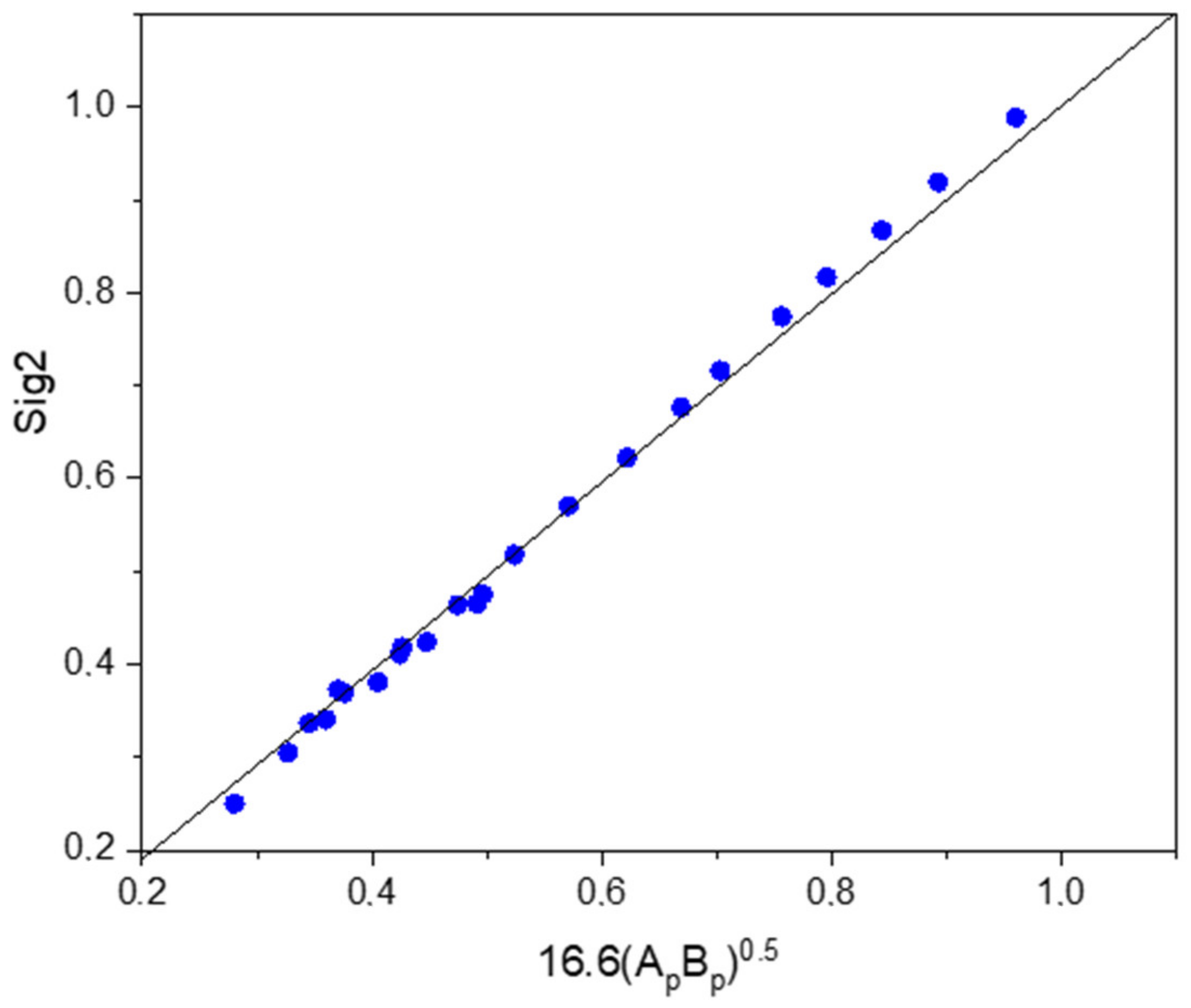
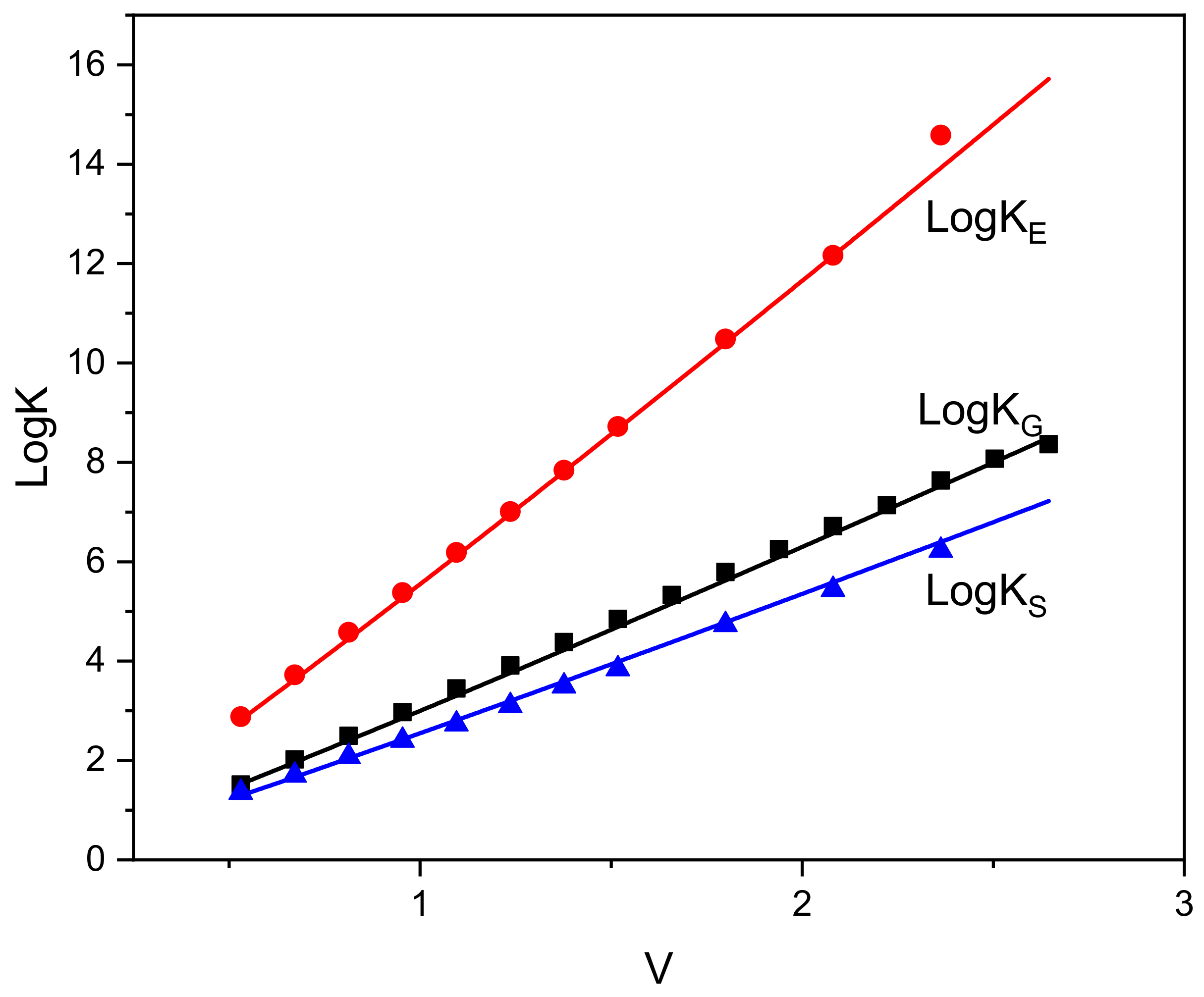
4.1. Self-Solvation Calculations
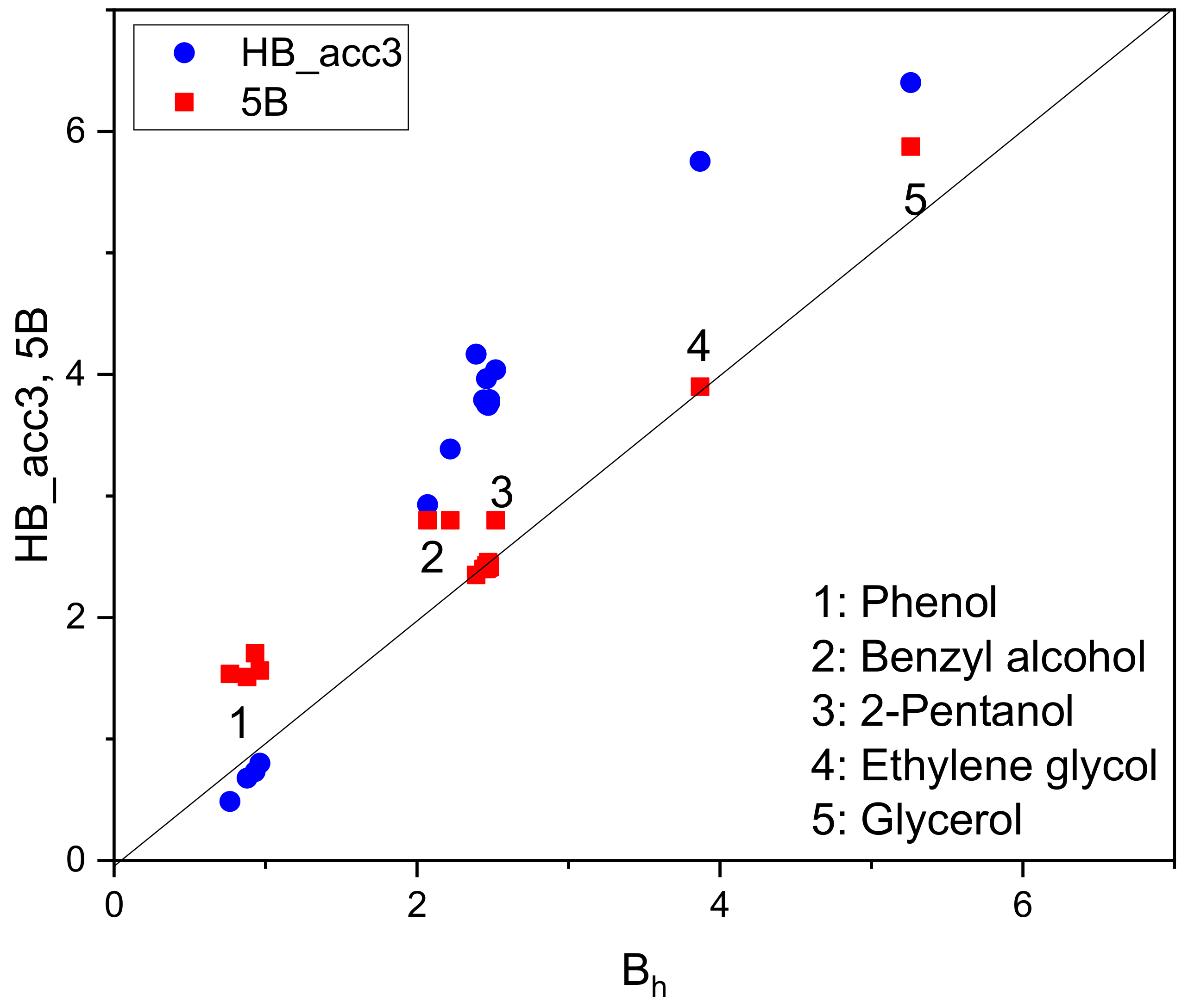
4.2. Hydrogen-Bonding Calculations in Solute (1)–Solvent (2) Systems
5. Discussion and Conclusions
Supplementary Materials
Funding
Data Availability Statement
Conflicts of Interest
References
- Moore, J.D.; Mountain, R.D.; Ross, R.B.; Shen, V.K.; Siderius, D.W.; Smith, K.D. The 9th Industrial Fluid Properties Simulation Challenge. Fluid Phase Equilib. 2018, 476, 1–5. [Google Scholar] [CrossRef] [PubMed]
- Tillotson, M.J.; Diamantonis, N.I.; Buda, C.; Bolton, L.W.; Müller, E.A. Molecular modelling of the thermophysical properties of fluids: Expectations, limitations, gaps and opportunities. Phys. Chem. Chem. Phys. 2023, 25, 12607–12628. [Google Scholar] [CrossRef]
- Sapir, L.; Harries, D. Revisiting Hydrogen Bond Thermodynamics in Molecular Simulations. J. Chem. Theory Comput. 2017, 13, 2851–2857. [Google Scholar] [CrossRef]
- Matos, G.D.R.; Kyu, D.Y.; Loeffler, H.H.; Chodera, J.D.; Shirts, M.R.; Mobley, D.L. Approaches for Calculating Solvation Free Energies and Enthalpies Demonstrated with an Update of the FreeSolv Database. J. Chem. Eng. Data 2017, 62, 1559–1569. [Google Scholar] [CrossRef]
- Hirata, F. Exploring Life Phenomena with Statistical Mechanics of Molecular Liquids; CRC Press: Boca Raton, FL, USA, 2020. [Google Scholar]
- Pereyaslavets, L.; Kamath, G.; Butin, O.; Illarionov, A.; Olevanov, M.; Kurnikov, I.; Sakipov, S.; Leontyev, I.; Voronina, E.; Gannon, T.; et al. Accurate determination of solvation free energies of neutral organic compounds from first principles. Nat. Commun. 2022, 13, 414. [Google Scholar] [CrossRef]
- Abraham, M.H.; McGowan, J.C. The use of characteristic volumes to measure cavity terms in reversed phase liquid chromatography. Chromatographia 1987, 23, 243–246. [Google Scholar] [CrossRef]
- Abraham, M.H. Scales of solute hydrogen-bonding: Their construction and application to physicochemical and biochemical processes. Chem. Soc. Rev. 1993, 22, 73–83. [Google Scholar] [CrossRef]
- Abraham, M.H.; Ibrahim, A.; Zissimos, A.M. Determination of sets of solute descriptors from chromatographic measurements. J. Chromatogr. A 2004, 1037, 29–47. [Google Scholar] [CrossRef]
- Abraham, M.H.; Smith, R.E.; Luchtefeld, R.; Boorem, A.J.; Luo, R.; Acree, W.E., Jr. Prediction of solubility of drugs and other compounds in organic solvents. J. Pharm. Sci. 2010, 99, 1500–1515. [Google Scholar] [CrossRef]
- Goss, K.-U. Predicting the equilibrium partitioning of organic compounds using just one linear solvation energy relationship (LSER). Fluid Phase Equilibria 2005, 233, 19–22. [Google Scholar] [CrossRef]
- Endo, S.; Watanabe, N.; Ulrich, N.; Bronner, G.K.-U. Goss UFZ-LSER Database v 2.1. Helmholtz Centre for Environmental Research-UFZ, Leipzig, Germany, 2015. Available online: https://www.ufz.de/index.php?en=31698&contentonly=1&m=0&lserd_data[mvc]=Public/start (accessed on 12 June 2024).
- Sinha, S.; Yang, C.; Wu, E.; Acree, W.E. Abraham Solvation Parameter Model: Examination of Possible Intramolecular Hydrogen-Bonding Using Calculated Solute Descriptors. Liquids 2022, 2, 131–146. [Google Scholar] [CrossRef]
- Mintz, C.; Ladlie, T.; Burton, K.; Clark, M.; Acree, W.E., Jr.; Abraham, M.H. Enthalpy of Solvation Correlations for Gaseous Solutes Dissolved in Alcohol Solvents based on the Abraham Model. QSAR Comb. Sci. 2008, 27, 627–635. [Google Scholar] [CrossRef]
- Egert, T.; Langowski, H.C. Linear Solvation Energy Relationships (LSERs) for Accurate Prediction of Partition Coefficients between Low Density Polyethylene and Water-Part II: Model Evaluation and Benchmarking. Eur. J. Pharm. Sci. 2022, 172, 106137. [Google Scholar] [CrossRef] [PubMed]
- Panayiotou, C.; Zuburtikudis, I.; Abu Khalifeh, H. Linear Free-Energy Relationships and Solvation Thermodynamics: The Thermodynamic Basis of LFER Linearity. Ind. Eng. Chem. Res. 2023, 62, 2989–3000. [Google Scholar] [CrossRef]
- Panayiotou, C.; Zuburtikudis, I.; Abu Khalifeh, H.; Hatzimanikatis, V. Linear Solvation–Energy Relationships (LSER) and Equation-of-State Thermodynamics: On the Extraction of Thermodynamic Information from the LSER Database. Liquids 2023, 3, 66–89. [Google Scholar] [CrossRef]
- Panayiotou, C.; Acree, W.E., Jr.; Zuburtikudis, I. COSMO-RS and LSER Models of Solution Thermodynamics: Towards a COSMOLSER Equation of State Model of Fluids. J. Molec. Liq. 2023, 390, 122992. [Google Scholar] [CrossRef]
- Moine, E.; Privat, R.; Sirjean, B.; Jaubert, J.-N. Estimation of Solvation Quantities from Experimental Thermodynamic Data: Development of the Comprehensive CompSol Databank for Pure and Mixed Solutes. J. Phys. Chem. Ref. Data 2017, 46, 033102. [Google Scholar] [CrossRef]
- Joesten, M.D.; Schaad, L. Hydrogen Bonding; Marcel Dekker: New York, NY, USA, 1974. [Google Scholar]
- Raevsky, O.A.; Grigor'Ev, V.Y.; Kireev, D.B.; Zefirov, N.S. Complete Thermodynamic Description of H-Bonding in the Framework of Multiplicative Approach. Quant. Struct. Relationships 1992, 11, 49–63. [Google Scholar] [CrossRef]
- Gilli, G.; Gilli, P. The Nature of the Hydrogen Bond; Oxford University Press: Oxford, UK, 2009. [Google Scholar]
- Baev, A.K. Specific Intermolecular Interactions of Nitrogenated and Bioorganic Compounds; Springer: Berlin/Heidelberg, Germany, 2014. [Google Scholar]
- Katritzky, A.R.; Fara, D.C.; Yang, H.; Tämm, K.; Tamm, T.; Karelson, M. Quantitative Measures of Solvent Polarity. Chem. Rev. 2004, 104, 175–198. [Google Scholar] [CrossRef]
- Laurence, C.; Gal, J.-F. Lewis Basicity and Affinity Scales: Data and Measurements; Wiley: New York, NY, USA, 2010. [Google Scholar]
- Epley, T.D.; Drago, R.S. Calorimetric studies on some hydrogen-bonded adducts. J. Am. Chem. Soc. 1967, 89, 5770–5773. [Google Scholar] [CrossRef]
- Murthy, A.S.; Rao, C. Spectroscopic Studies of the Hydrogen Bond. Appl. Spectrosc. Rev. 1968, 2, 69–191. [Google Scholar] [CrossRef]
- Arnett, E.M.; Joris, L.; Mitchell, E.; Murty, T.; Gorrie, T.; Schleyer, P.V.R. Hydrogen-bonded complex formation. III. Thermodynamics of complexing by infrared spectroscopy and calorimetry. J. Am. Chem. Soc. 1970, 92, 2365–2377. [Google Scholar] [CrossRef]
- Cabani, S.; Gianni, P.; Mollica, V.; Lepori, L. Group Contributions to the Thermodynamic Properties of Non-Ionic Organic Solutes in Dilute Aqueous Solution. J. Solut. Chem. 1981, 10, 563–595. [Google Scholar] [CrossRef]
- Abbott, S.; Yamamoto, H.; Hansen, C.M. Hansen Solubility Parameters in Practice, Complete with Software, Data and Examples, 3rd ed.; version 3.1.20; Hansen-Solubility: Hørsholm, Denmark, 2010. [Google Scholar]
- Dortmund Data Bank. Available online: https://www.ddbst.com/ddb.html (accessed on 28 June 2024).
- Sedov, L.A.; Solomonov, B.N. Hydrogen bonding in neat aliphatic alcohols: The Gibbs free energy of self-association and molar fraction of monomer. J. Mol. Liq. 2012, 167, 47–51. [Google Scholar] [CrossRef]
- Solomonov, B.N.; Yagofarov, M.I. Compensation relationship in thermodynamics of solvation and vaporization: Features and applications. I. Non-hydrogen-bonded systems. J. Mol. Liq. 2022, 368, 120762. [Google Scholar] [CrossRef]
- Solomonov, B.N.; Yagofarov, M.I. Compensation relationship in thermodynamics of solvation and vaporization: Features and applications. II. Hydrogen-bonded systems. J. Mol. Liq. 2023, 372, 121205. [Google Scholar] [CrossRef]
- Dohnal, V. New QSPR molecular descriptors based on low-cost quantum chemistry computations using DFT/COSMO approach. J. Mol. Liq. 2024, 407, 125256. [Google Scholar] [CrossRef]
- Goodsell, D.S. Bionanotechnology: Lessons from Nature; Wiley & Sons: New York, NY, USA, 2003. [Google Scholar]
- Qiu, X.; Li, H.; Ver Steeg, G.; Godzik, A. Advances in AI for Protein Structure Prediction: Implications for Cancer Drug Discovery and Development. Biomolecules 2024, 14, 339. [Google Scholar] [CrossRef]
- Chapman, W.G.; Gubbins, K.E.; Jackson, G.; Radosz, M. New reference equation of state for associating liquids. Ind. Eng.Chem. Res. 1990, 29, 1709–1721. [Google Scholar] [CrossRef]
- Vega, L.; Llovell, F. Review and new insights into the application of molecular-based equations of state to water and aqueous solutions. Fluid Phase Equilibria 2016, 416, 150–173. [Google Scholar] [CrossRef]
- Torshizi, M.F.; Muller, E.A. Coarse-grained molecular dynamics study of the self-assembly of polyphilic bolaamphiphiles using the SAFT-γ Mie force field. Mol. Syst. Des. Eng. 2021, 6, 594–608. [Google Scholar] [CrossRef]
- Wertheim, M. Fluids with highly directional attractive forces. III. Multiple attraction sites. J. Statist. Phys. 1986, 42, 459–476. [Google Scholar] [CrossRef]
- Kontogeorgis, G.M.; Folas, G.K. Thermodynamic Models for Industrial Applications. From Classical and Advanced Mixing Rules to Association Theories; John Wiley and Sons, Ltd.: Chichester, UK, 2010. [Google Scholar]
- Panayiotou, C.; Sanchez, I.C. Hydrogen Bonding in Fluids: An Equation of-State Approach. J. Phys. Chem. 1991, 95, 10090–10097. [Google Scholar] [CrossRef]
- Panayiotou, C.; Pantoula, M.; Stefanis, E.; Tsivintzelis, I.; Economou, I.G. Nonrandom Hydrogen-Bonding Model of Fluids and Their Mixtures. 1. Pure Fluids. Ind. Eng. Chem. Res. 2004, 43, 6592–6606. [Google Scholar] [CrossRef]
- Panayiotou, C.; Tsivintzelis, I.; Economou, I.G. Nonrandom Hydrogen-Bonding Model of Fluids and Their Mixtures. 2. Multicomponent Mixtures. Ind. Eng. Chem. Res. 2007, 46, 2628–2636. [Google Scholar] [CrossRef]
- Veytsman, B.A. Are lattice models valid for fluids with hydrogen bonds? J. Phys. Chem. 1990, 94, 8499–8500. [Google Scholar] [CrossRef]
- Mensitieri, G.; Scherillo, G.; Panayiotou, C.; Musto, P. Towards a predictive thermodynamic description of sorption processes in polymers: The synergy between theoretical EoS models and vibrational spectroscopy. Mater. Sci. Eng. R Rep. 2020, 140, 100525. [Google Scholar] [CrossRef]
- Klamt, A. Conductor-like Screening Model for Real Solvents: A New Approach to the Quantitative Calculation of Solvation Phenomena. J. Phys. Chem. 1995, 99, 2224–2235. [Google Scholar] [CrossRef]
- Lin, S.-T.; Sandler, S.I. A Priori Phase Equilibrium Prediction from a Segment Contribution Solvation Model. Ind. Eng. Chem. Res. 2001, 41, 899–913. [Google Scholar] [CrossRef]
- Bell, I.H.; Mickoleit, E.; Hsieh, C.-M.; Lin, S.-T.; Vrabec, J.; Breitkopf, C.; Jäger, A. A Benchmark Open-Source Implementation of COSMO-SAC. J. Chem. Theory Comput. 2020, 16, 2635–2646. [Google Scholar] [CrossRef]
- Klamt, A. COSMO-RS from Quantum Chemistry to Fluid Phase Thermodynamics and Drug Design; Elsevier: Amsterdam, The Netherlands, 2005. [Google Scholar]
- Grensemann, H.; Gmehling, J. Performance of a Conductor-Like Screening Model for Real Solvents Model in Comparison to Classical Group Contribution Methods. Ind. Eng. Chem. Res. 2005, 44, 1610–1624. [Google Scholar] [CrossRef]
- Pye, C.C.; Ziegler, T.; van Lenthe, E.; Louwen, J.N. An implementation of the conductor-like screening model of solvation within the Amsterdam density functional package—Part II. COSMO for real solvents. Can. J. Chem. 2009, 87, 790–797. [Google Scholar] [CrossRef]
- Klamt, A.; Eckert, F.; Arlt, W. COSMO-RS: An Alternative to Simulation for Calculating Thermodynamic Properties of Liquid Mixtures. Annu. Rev. Chem. Biomol. Eng. 2010, 1, 101–122. [Google Scholar] [CrossRef] [PubMed]
- Klamt, A.; Eckert, F.; Reinisch, J.; Wichmann, K. Prediction of cyclohexane-water distribution coefficients with COSMO-RS on the SAMPL5 data set. J. Comput. Aided Mol. Des. 2016, 30, 959–967. [Google Scholar] [CrossRef]
- Reinisch, J.; Klamt, A. Prediction of free energies of hydration with COSMO-RS on the SAMPL4 data set. J. Comput. Aided Mol. Des. 2014, 28, 169–173. [Google Scholar] [CrossRef]
- North Data. COSMObase, Ver. 2019; COSMOlogic GmbH & CoKG: Leverkusen, Germany; BIOVIA Dassault Systemes: Waltham, MA, USA, 2019. [Google Scholar]
- Zissimos, A.M.; Abraham, M.H.; Klamt, A.; Eckert, F.; Wood, J. A Comparison between the Two General Sets of Linear Free Energy Descriptors of Abraham and Klamt. J. Chem. Inf. Comput. Sci. 2002, 42, 1320–1331. [Google Scholar] [CrossRef]
- Program Package for Electronic Structure Calculations. Available online: https://www.turbomole.org (accessed on 28 September 2024).
- Modeling & Simulation for Next-Generation Materials. Available online: https://www.3ds.com/products/biovia/materials-studio (accessed on 28 September 2024).
- What is COSMO-RS/SAC. Available online: https://www.scm.com/product/cosmo-rs/ (accessed on 28 September 2024).
- Missopolinou, D.; Ioannou, K.; Prinos, I.; Panayiotou, C. Thermodynamics of Alkoxyethanol + Alkane Mixtures. Z. Phys. Chem. 2002, 216, 905. [Google Scholar] [CrossRef]
- Missopolinou, D.; Tsivintzelis, I.; Panayiotou, C. Excess enthalpies of binary mixtures of 2-ethoxyethanol with four hydrocarbons at 298.15, 308.15, and 318.15K: An experimental and theoretical study. Fluid Phase Equilibria 2006, 245, 89–101. [Google Scholar] [CrossRef]


| SOLUTE | Ah | Ap | Bp | Bh |
|---|---|---|---|---|
| ETHANE | 0.00 | 0.28 | 0.23 | 0.00 |
| PROPANE | 0.00 | 0.32 | 0.29 | 0.00 |
| n-BUTANE | 0.00 | 0.37 | 0.37 | 0.00 |
| n-PENTANE | 0.00 | 0.42 | 0.40 | 0.00 |
| n-HEXANE | 0.00 | 0.47 | 0.46 | 0.00 |
| n-HEPTANE | 0.00 | 0.52 | 0.52 | 0.00 |
| n-OCTANE | 0.00 | 0.57 | 0.57 | 0.00 |
| n-NONANE | 0.00 | 0.62 | 0.63 | 0.00 |
| n-DECANE | 0.00 | 0.67 | 0.69 | 0.00 |
| n-UNDECANE | 0.00 | 0.71 | 0.73 | 0.00 |
| n-DODECANE | 0.00 | 0.77 | 0.78 | 0.00 |
| n-TRIDECANE | 0.00 | 0.80 | 0.84 | 0.00 |
| n-TETRADECANE | 0.00 | 0.85 | 0.89 | 0.00 |
| n-PENTADECANE | 0.00 | 0.90 | 0.94 | 0.00 |
| n-HEXADECANE | 0.00 | 0.96 | 1.02 | 0.00 |
| n-OCTADECANE | 0.00 | 1.05 | 1.11 | 0.00 |
| ISOBUTANE | 0.00 | 0.39 | 0.37 | 0.00 |
| ISOPENTANE | 0.00 | 0.44 | 0.41 | 0.00 |
| 2-METHYLPENTANE | 0.00 | 0.49 | 0.46 | 0.00 |
| 3-METHYLPENTANE | 0.00 | 0.49 | 0.45 | 0.00 |
| 3-METHYLHEXANE | 0.00 | 0.54 | 0.51 | 0.00 |
| 2,2-DIMETHYLHEXANE | 0.00 | 0.61 | 0.60 | 0.00 |
| 2,5-DIMETHYLHEXANE | 0.00 | 0.59 | 0.58 | 0.00 |
| CYCLOPENTANE | 0.00 | 0.35 | 0.33 | 0.00 |
| CYCLOHEXANE | 0.00 | 0.35 | 0.33 | 0.00 |
| CYCLOHEPTANE | 0.00 | 0.38 | 0.37 | 0.00 |
| CYCLOOCTANE | 0.00 | 0.42 | 0.42 | 0.00 |
| ETHYLENE | 0.00 | 0.67 | 0.73 | 0.02 |
| PROPYLENE | 0.00 | 0.67 | 0.80 | 0.06 |
| 1-BUTENE | 0.00 | 0.70 | 0.84 | 0.06 |
| 1-PENTENE | 0.00 | 0.74 | 0.90 | 0.07 |
| 1-HEXENE | 0.00 | 0.79 | 0.96 | 0.06 |
| 1-HEPTENE | 0.00 | 0.83 | 1.02 | 0.06 |
| 1-OCTENE | 0.00 | 0.86 | 1.07 | 0.05 |
| BENZENE | 0.00 | 1.24 | 1.14 | 0.00 |
| TOLUENE | 0.00 | 1.22 | 1.23 | 0.00 |
| ETHYLBENZENE | 0.00 | 1.25 | 1.29 | 0.00 |
| n-PROPYLBENZENE | 0.00 | 1.29 | 1.36 | 0.00 |
| n-BUTYLBENZENE | 0.00 | 1.34 | 1.42 | 0.00 |
| o-XYLENE | 0.00 | 1.25 | 1.34 | 0.00 |
| m-XYLENE | 0.00 | 1.22 | 1.31 | 0.00 |
| p-XYLENE | 0.00 | 1.21 | 1.29 | 0.00 |
| 1-PENTYNE | 0.49 | 1.01 | 1.51 | 0.16 |
| 1-HEXYNE | 0.48 | 1.05 | 1.57 | 0.17 |
| 3-HEXYNE | 0.00 | 1.10 | 1.39 | 0.34 |
| DICHLOROMETHANE | 0.94 | 0.94 | 1.08 | 0.00 |
| CHLOROFORM | 1.14 | 0.59 | 0.71 | 0.00 |
| CARBON TETRACHLORIDE | 0.00 | 0.71 | 0.37 | 0.00 |
| 2,2-DICHLOROPROPANE | 0.00 | 1.48 | 1.43 | 0.00 |
| CARBON TETRAFLUORIDE | 0.00 | 0.33 | 0.14 | 0.00 |
| DIETHYL ETHER | 0.00 | 0.79 | 0.38 | 1.81 |
| DI-n-PROPYL ETHER | 0.00 | 0.85 | 0.47 | 1.79 |
| DI-n-BUTYL ETHER | 0.00 | 0.94 | 0.60 | 1.79 |
| FURAN | 0.24 | 1.40 | 1.24 | 0.13 |
| TETRAHYDROFURAN | 0.00 | 0.79 | 0.31 | 2.15 |
| 1,3-DIOXANE | 0.00 | 1.50 | 0.54 | 3.12 |
| 1,4-DIOXANE | 0.00 | 1.50 | 0.54 | 3.12 |
| TETRAHYDROPYRAN | 0.00 | 0.77 | 0.34 | 1.97 |
| METHYL FORMATE | 0.19 | 1.59 | 0.74 | 2.21 |
| ETHYL FORMATE | 0.15 | 1.56 | 0.73 | 2.36 |
| ETHYL ACETATE | 0.00 | 1.61 | 0.68 | 2.81 |
| n-PROPYL ACETATE | 0.00 | 1.60 | 0.72 | 2.80 |
| ISOPROPYL ACETATE | 0.00 | 1.65 | 0.68 | 2.68 |
| n-BUTYL ACETATE | 0.00 | 1.64 | 0.76 | 2.81 |
| ETHYL PROPIONATE | 0.00 | 1.53 | 0.73 | 2.66 |
| ETHYL n-BUTYRATE | 0.00 | 1.56 | 0.78 | 2.65 |
| n-PROPYL PROPIONATE | 0.00 | 1.54 | 0.74 | 2.69 |
| ACETONE | 0.02 | 1.47 | 0.38 | 2.95 |
| METHYL ETHYL KETONE | 0.00 | 1.41 | 0.43 | 2.78 |
| 2-PENTANONE | 0.00 | 1.43 | 0.47 | 2.81 |
| 3-PENTANONE | 0.00 | 1.35 | 0.51 | 2.58 |
| 3-HEXANONE | 0.00 | 1.37 | 0.53 | 2.62 |
| FORMALDEHYDE | 0.00 | 1.34 | 0.62 | 1.55 |
| ACETALDEHYDE | 0.00 | 1.39 | 0.47 | 2.36 |
| PROPANAL | 0.00 | 1.32 | 0.49 | 2.33 |
| BUTANAL | 0.00 | 1.34 | 0.54 | 2.32 |
| PENTANAL | 0.00 | 1.38 | 0.59 | 2.33 |
| HEXANAL | 0.00 | 1.43 | 0.66 | 2.32 |
| OCTANAL | 0.00 | 1.52 | 0.76 | 2.33 |
| METHANOL | 1.39 | 0.55 | 0.29 | 2.39 |
| ETHANOL | 1.23 | 0.66 | 0.35 | 2.46 |
| 1-PROPANOL | 1.23 | 0.70 | 0.41 | 2.44 |
| 1-BUTANOL | 1.22 | 0.74 | 0.44 | 2.47 |
| 1-PENTANOL | 1.22 | 0.79 | 0.51 | 2.46 |
| 1-HEXANOL | 1.22 | 0.83 | 0.55 | 2.48 |
| 1-HEPTANOL | 1.21 | 0.90 | 0.61 | 2.48 |
| 1-OCTANOL | 1.19 | 0.95 | 0.68 | 2.46 |
| 1-NONANOL | 1.21 | 0.99 | 0.73 | 2.47 |
| 1-DECANOL | 1.23 | 1.02 | 0.79 | 2.47 |
| ISOPROPANOL | 1.18 | 0.73 | 0.38 | 2.52 |
| 2-BUTANOL | 0.91 | 0.81 | 0.39 | 2.46 |
| 2-PENTANOL | 1.14 | 0.79 | 0.52 | 2.22 |
| GLYCEROL | 2.98 | 1.68 | 0.75 | 5.26 |
| ETHYLENE GLYCOL, c0 | 2.13 | 1.10 | 0.57 | 3.87 |
| ETHYLENE GLYCOL, c6 Econf = 8.98 | 2.97 | 0.86 | 0.86 | 4.11 |
| 1,3-PROPYLENE GLYCOL, c0 | 1.58 | 1.17 | 0.53 | 3.92 |
| 1,3-PROPYLENE GLYCOL, c3 Econf = 5.54 | 2.63 | 1.01 | 0.56 | 4.38 |
| 1,2-BUTANEDIOL | 1.73 | 1.20 | 0.64 | 3.66 |
| 1,3-BUTANEDIOL | 1.60 | 1.21 | 0.58 | 3.96 |
| 1,4-BUTANEDIOL | 1.63 | 1.08 | 0.55 | 3.98 |
| 2-METHOXYETHANOL c0 | 0.77 | 1.22 | 0.60 | 3.13 |
| 2-METHOXYETHANOL c7 Econf = 10.97 | 1.39 | 1.08 | 0.62 | 3.19 |
| 2-ETHOXYETHANOL c0 | 0.63 | 1.24 | 0.60 | 3.13 |
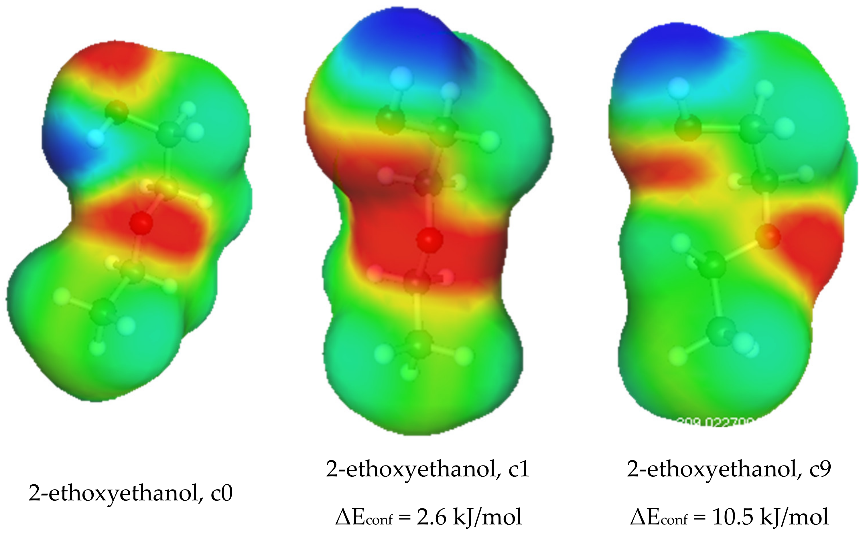
| 2-ETHOXYETHANOL c1 Econf = 2.59 | 1.35 | 1.20 | 0.47 | 4.23 |
| 2-ETHOXYETHANOL c9 Econf = 10.5 | 1.39 | 1.11 | 0.64 | 3.28 |
| PHENOL | 2.03 | 1.26 | 1.45 | 0.88 |
| o-CRESOL | 1.99 | 1.21 | 1.57 | 0.77 |
| m-CRESOL | 1.98 | 1.25 | 1.52 | 0.93 |
| p-CRESOL | 1.96 | 1.26 | 1.46 | 0.96 |
| BENZYL ALCOHOL | 1.23 | 1.59 | 1.18 | 2.07 |
| ACETIC ACID | 2.04 | 1.11 | 0.76 | 2.70 |
| PROPIONIC ACID | 1.99 | 1.06 | 0.78 | 2.62 |
| n-BUTYRIC ACID | 1.98 | 1.07 | 0.83 | 2.62 |
| n-PENTANOIC ACID | 1.97 | 1.12 | 0.89 | 2.62 |
| ETHYLAMINE | 0.43 | 0.95 | 0.32 | 2.73 |
| n-BUTYLAMINE | 0.43 | 1.04 | 0.45 | 2.73 |
| DIETHYLAMINE | 0.20 | 0.84 | 0.40 | 2.02 |
| DI-n-PROPYLAMINE | 0.19 | 0.93 | 0.52 | 2.02 |
| TRIMETHYLAMINE | 0.00 | 0.65 | 0.35 | 1.49 |
| ANILINE | 1.62 | 1.41 | 1.82 | 0.78 |
| PYRIDINE | 0.00 | 1.60 | 0.56 | 2.11 |
| FORMAMIDE | 3.03 | 0.84 | 0.36 | 4.23 |
| DIMETHYL SULFOXIDE | 0.10 | 2.30 | 0.29 | 5.24 |
| ACETONITRILE | 0.31 | 1.67 | 0.91 | 2.00 |
| ACRYLONITRILE | 0.43 | 1.48 | 1.00 | 1.52 |
| PROPIONITRILE | 0.08 | 1.64 | 0.91 | 2.02 |
| ACETAMIDE | 2.61 | 1.03 | 0.34 | 4.74 |
| N,N-DIMETHYLFORMAMIDE | 0.00 | 1.66 | 0.25 | 4.17 |
| N-METHYL FORMAMIDE | 1.58 | 1.21 | 0.28 | 4.20 |
| WATER | 2.89 | 0.28 | 0.27 | 2.99 |
| Solute | LogKS exp [19] | LogKS Equation (18) |
|---|---|---|
| ISOBUTANE | 1.57 | 1.63 |
| ISOPENTANE | 1.99 | 2.00 |
| 2-METHYLPENTANE | 2.25 | 2.38 |
| 3-METHYLPENTANE | 2.25 | 2.38 |
| 1-BUTENE | 1.62 | 1.65 |
| 1-PENTENE | 1.99 | 2.00 |
| 1-HEXENE | 2.38 | 2.35 |
| 3-HEXYNE | 2.40 | 2.40 |
| CYCLOPENTANE | 2.03 | 2.00 |
| CYCLOHEXANE | 2.25 | 2.33 |
| CYCLOHEPTANE | 2.64 | 2.67 |
| CYCLOOCTANE | 2.95 | 3.03 |
| BENZENE | 2.36 | 2.32 |
| TOLUENE | 2.58 | 2.61 |
| ETHYLBENZENE | 2.93 | 2.92 |
| n-PROPYLBENZENE | 3.19 | 3.25 |
| n-BUTYLBENZENE | 3.58 | 3.60 |
| o-XYLENE | 2.99 | 2.92 |
| m-XYLENE | 2.92 | 2.92 |
| p-XYLENE | 2.93 | 2.92 |
| CARBON TETRACHLORIDE | 2.23 | 2.23* |
| DIETHYL ETHER | 2.21 | 2.00 |
| DI-n-PROPYL ETHER | 2.67 | 2.69 |
| DI-n-BUTYL ETHER | 3.39 | 3.42 |
| ETHYL ACETATE | 2.71 | 2.59 |
| n-BUTYL ACETATE | 3.41 | 3.16 |
| ACETONE | 2.27 | 2.10 |
| METHYL ETHYL KETONE | 2.49 | 2.33 |
| 2-PENTANONE | 2.80 | 2.60 |
| 3-PENTANONE | 2.60 | 2.60 |
| ACETALDEHYDE | 2.01 | 1.96 |
| PROPANAL | 2.21 | 2.10 |
| BUTANAL | 2.34 | 2.33 |
| PENTANAL | 2.51 | 2.60 |
| HEXANAL | 2.88 | 2.90 |
| Solute | LogKS exp [19] | LogKS,nhb Equation (18) | LogKS,hb | −ΔSHB/ JK−1 mol−1 | −ΔHHB [57] kJmol−1 | −ΔGHB/ kJmol−1 Equation (20) | −ΔGHB/ kJmol−1 LSER [13] |
|---|---|---|---|---|---|---|---|
| METHANOL | 2.95 | 0.88 | 2.07 | 39.58 | 23.08 | 11.28 | 13.14 |
| ETHANOL | 3.47 | 1.40 | 2.08 | 39.78 | 24.93 | 13.07 | 11.49 |
| 1-PROPANOL | 4.02 | 1.68 | 2.34 | 44.78 | 24.61 | 11.26 | 11.16 |
| 2-PROPANOL | 4.06 | 1.68 | 2.38 | 45.62 | 23.74 | 10.14 | 10.43 |
| 1-BUTANOL | 4.55 | 2.01 | 2.54 | 48.72 | 24.16 | 9.63 | 10.21 |
| 1-PENTANOL | 4.79 | 2.34 | 2.45 | 46.85 | 24.01 | 10.04 | 10.59 |
| 2-PENTANOL | 4.76 | 2.34 | 2.42 | 46.43 | 23.77 | 9.93 | 10.34 |
| 1-HEXANOL | 5.44 | 2.69 | 2.75 | 52.67 | 24.24 | 8.54 | 10.06 |
| 1-HEPTANOL | 6.01 | 3.05 | 2.96 | 56.64 | 23.64 | 6.75 | 9.77 |
| 1-OCTANOL | 6.14 | 3.42 | 2.72 | 52.10 | 23.43 | 7.90 | 9.40 |
| 1-NONANOL | 6.75 | 3.79 | 2.96 | 56.68 | 23.68 | 6.78 | |
| 1-DECANOL | 6.84 | 4.17 | 2.67 | 51.11 | 23.26 | 8.02 | 9.40 |
| ETHYLENE GLYCOL, c0 | 4.68 | 1.77 | 2.91 | 54.51 | 43.29 | 26.70 | 25.24 |
| 1,3-PROPYLENE GLYCOL, c0 | 4.74 | 2.02 | 2.72 | 51.10 | 50.21 | 34.70 | |
| GLYCEROL | 6.18 | 2.32 | 3.86 | 73.90 | 51.61 | 29.58 | |
| BENZYL ALCOHOL | 4.87 | 2.88 | 2.00 | 38.25 | 22.47 | 11.06 | 10.32 |
| PHENOL | 4.26 | 2.59 | 1.67 | 31.91 | 17.58 | 8.07 | |
| o-CRESOL | 4.55 | 2.88 | 1.67 | 31.98 | 13.22 | 3.69 | |
| m-CRESOL | 4.63 | 2.88 | 1.76 | 33.65 | 17.98 | 7.95 | |
| p-CRESOL | 4.96 | 2.88 | 2.09 | 39.92 | 18.59 | 6.69 | |
| 2-METHOXY-ETHANOL c0 | 3.28 | 2.03 | 1.25 | 23.99 | 19.53 | 12.38 | 9.06 |
| 2-ETHOXY-ETHANOL c0 | 3.93 | 2.32 | 1.61 | 30.89 | 19.21 | 10.00 | 9.45 |
| ACETIC ACID | 2.69 | 1.84 | 0.85 | 16.27 | 25.31 | 20.46 | 14.95 |
| PROPIONIC ACID | 3.43 | 2.05 | 1.38 | 26.43 | 25.39 | 17.51 | |
| n-BUTYRIC ACID | 4.09 | 2.32 | 1.77 | 33.84 | 25.37 | 15.28 | |
| n-PENTANOIC ACID | 4.85 | 2.62 | 2.23 | 42.71 | 24.89 | 12.16 | |
| n-BUTYLAMINE | 2.69 | 2.00 | 0.69 | 13.19 | 2.84 | −1.10 | |
| DIETHYLAMINE | 2.38 | 2.00 | 0.38 | 7.33 | 2.69 | 0.50 | |
| WATER | 2.72 | 0.38 | 2.35 | 44.77 | 41.15 | 27.80 | 27.37 |
| SOLUTE | LSER [13,14] | This Work / COSMO-RS [57] | |||
|---|---|---|---|---|---|
| −A1a2/ kJ/mol | −B1b2/ kJ/mol | ch12 | −ch12Ah1Bh2 / kJ/mol | −ch12BBh1Ah2 / kJ/mol | |
| Solvent: WATER | |||||
| WATER | 24.41 | 15.79 | 0.42 | 20.56 | 20.56 |
| TETRAHYDROFURAN | 0.00 | 20.03 | 0.69 | 0.00 | 24.52 |
| TETRAHYDROPYRAN | 0.00 | 21.43 | 0.72 | 0.00 | 23.26 |
| ETHYL ACETATE | 0.00 | 18.82 | 0.38 | 0.00 | 17.59 |
| n-PROPYL ACETATE | 0.00 | 18.82 | 0.38 | 0.00 | 17.61 |
| n-BUTYL ACETATE | 0.00 | 18.79 | 0.39 | 0.00 | 18.03 |
| ACETONE | 1.28 | 20.62 | 0.40 | 0.14 | 19.52 |
| METHYL ETHYL KETONE | 0.00 | 21.31 | 0.41 | 0.00 | 18.64 |
| 2-PENTANONE | 0.00 | 21.30 | 0.42 | 0.00 | 19.64 |
| ACETALDEHYDE | 0.00 | 18.82 | 0.35 | 0.00 | 13.60 |
| PROPANAL | 0.00 | 18.82 | 0.35 | 0.00 | 13.48 |
| BUTANAL | 0.00 | 18.82 | 0.35 | 0.00 | 13.51 |
| DMSO | 0.00 | 38.05 | 0.32 | 0.57 | 27.81 |
| METHANOL | 13.76 | 19.65 | 0.49 | 11.53 | 19.17 |
| ETHANOL | 11.84 | 20.07 | 0.55 | 11.63 | 22.48 |
| 1-PROPANOL | 11.84 | 20.07 | 0.56 | 11.61 | 22.35 |
| 1-BUTANOL | 11.80 | 20.16 | 0.55 | 11.51 | 22.52 |
| 1-PENTANOL | 11.80 | 20.16 | 0.56 | 11.56 | 22.53 |
| 1-HEXANOL | 11.76 | 20.29 | 0.55 | 11.48 | 22.55 |
| 1-HEPTANOL | 11.78 | 20.19 | 0.55 | 11.40 | 22.59 |
| 1-OCTANOL | 11.71 | 20.31 | 0.56 | 11.33 | 22.64 |
| 1-NONANOL | 11.76 | 20.53 | 0.56 | 11.51 | 22.71 |
| 1-DECANOL | 11.66 | 20.37 | 0.56 | 11.70 | 22.71 |
| ISOPROPANOL | 9.81 | 23.42 | 0.60 | 11.99 | 24.74 |
| 2-PENTANOL | 10.44 | 23.42 | 0.64 | 12.38 | 23.31 |
| PHENOL | 19.50 | 12.63 | 0.50 | 17.17 | 7.18 |
| ETHYLENE GLYCOL, c0 | 18.57 | 32.62 | 0.63 | 23.08 | 40.54 |
| ETHYLENE GLYCOL, c6 | 18.57 | 32.62 | 0.54 | 27.23 | 36.39 |
| 2-ETHOXYETHANOL c0 | 9.72 | 34.10 | 0.89 | 9.56 | 45.97 |
| 2-ETHOXYETHANOL c1 | 9.72 | 34.10 | 0.60 | 13.74 | 41.79 |
| 2-ETHOXYETHANOL c9 | 9.72 | 34.10 | 0.71 | 16.90 | 38.63 |
| 1,2-BUTANEDIOL | 18.57 | 35.13 | 0.65 | 19.28 | 39.46 |
| 1,3-BUTANEDIOL | 20.65 | 35.13 | 0.71 | 19.52 | 46.63 |
| ACETIC ACID | 19.71 | 18.46 | 0.42 | 14.65 | 18.74 |
| PROPIONIC ACID | 19.42 | 18.54 | 0.44 | 15.12 | 19.23 |
| n-BUTYLAMINE | 5.12 | 25.51 | 0.41 | 2.98 | 18.35 |
| DIETHYLAMINE | 2.56 | 28.73 | 0.65 | 2.22 | 21.53 |
| PYRIDINE | 0.00 | 21.42 | 0.47 | 0.00 | 16.23 |
| Solvent: ETHANOL | |||||
| ETHANOL | 18.08 | 5.53 | 0.73 | 12.58 | 12.58 |
| 1-PROPANOL | 18.08 | 5.53 | 0.72 | 12.28 | 12.36 |
| 2-PROPANOL | 14.97 | 6.45 | 0.77 | 12.56 | 13.55 |
| 1-OCTANOL | 17.87 | 5.59 | 0.74 | 12.17 | 12.71 |
| ETHYLENE GLYCOL, c0 | 28.34 | 8.98 | 0.70 | 20.75 | 19.05 |
| ETHYLENE GLYCOL, c6 | 28.34 | 8.98 | 0.57 | 23.43 | 16.37 |
| 2-ETHOXYETHANOL c0 | 14.83 | 9.39 | 0.86 | 7.53 | 18.93 |
| 2-ETHOXYETHANOL c1 | 14.83 | 9.39 | 0.55 | 10.22 | 16.24 |
| 2-ETHOXYETHANOL c9 | 14.83 | 9.39 | 0.63 | 12.05 | 14.41 |
| ACETIC ACID | 30.08 | 5.08 | 0.47 | 13.39 | 8.96 |
| n-BYTYL AMINE | 7.82 | 7.02 | 0.82 | 4.87 | 15.69 |
| DMSO | 0.00 | 10.48 | 0.54 | 0.77 | 19.88 |
| WATER | 37.25 | 4.35 | 0.60 | 24.22 | 12.66 |
| Solvent: 1-OCTANOL | |||||
| 1-OCTANOL | 19.74 | 4.37 | 0.70 | 11.69 | 11.69 |
| ETHANOL | 19.98 | 4.32 | 0.69 | 11.91 | 11.52 |
| 1-PROPANOL | 19.98 | 4.32 | 0.73 | 12.55 | 12.09 |
| 2-PROPANOL | 16.54 | 5.03 | 0.74 | 12.19 | 12.59 |
| ETHYLENE GLYCOL, c0 | 31.31 | 7.01 | 0.65 | 19.52 | 17.15 |
| ETHYLENE GLYCOL, c6 | 31.31 | 7.01 | 0.53 | 21.97 | 14.70 |
| 2-ETHOXYETHANOL c0 | 16.39 | 7.33 | 0.77 | 6.80 | 16.37 |
| 2-ETHOXYETHANOL c1 | 16.39 | 7.33 | 0.49 | 9.19 | 13.98 |
| 2-ETHOXYETHANOL c9 | 16.39 | 7.33 | 0.56 | 10.81 | 12.36 |
| ACETIC ACID | 33.24 | 3.97 | 0.47 | 13.37 | 8.56 |
| n-BYTYL AMINE | 8.64 | 5.48 | 0.83 | 4.98 | 15.35 |
| DMSO | 0.00 | 8.18 | 0.54 | 0.77 | 19.06 |
| WATER | 41.17 | 3.39 | 0.59 | 23.80 | 11.91 |
| Solvent: DMSO | |||||
| DMSO (Dimethyl Sulfoxide) | 0.00 | 5.33 | 0.004 | 0.01 | 0.01 |
| ETHANOL | 17.55 | 2.81 | 0.36 | 13.17 | 0.52 |
| 1-PROPANOL | 17.55 | 2.81 | 0.36 | 13.08 | 0.51 |
| 1-OCTANOL | 17.34 | 2.85 | 0.36 | 12.94 | 0.53 |
| 2-PROPANOL | 14.53 | 3.28 | 0.36 | 12.54 | 0.53 |
| ETHYLENE GLYCOL, c0 | 27.50 | 4.57 | 0.41 | 25.79 | 0.92 |
| ETHYLENE GLYCOL, c6 | 27.50 | 4.57 | 0.29 | 26.00 | 0.71 |
| 2-ETHOXYETHANOL c0 | 14.39 | 4.78 | 0.62 | 11.62 | 1.14 |
| 2-ETHOXYETHANOL c1 | 14.39 | 4.78 | 0.30 | 12.02 | 0.74 |
| 2-ETHOXYETHANOL c9 | 14.39 | 4.78 | 0.29 | 12.19 | 0.57 |
| ACETIC ACID | 29.20 | 2.59 | 0.31 | 18.81 | 0.49 |
| n-BYTYL AMINE | 7.59 | 3.58 | 0.04 | 0.50 | 0.06 |
| WATER | 36.16 | 2.21 | 0.33 | 28.28 | 0.58 |
Disclaimer/Publisher’s Note: The statements, opinions and data contained in all publications are solely those of the individual author(s) and contributor(s) and not of MDPI and/or the editor(s). MDPI and/or the editor(s) disclaim responsibility for any injury to people or property resulting from any ideas, methods, instructions or products referred to in the content. |
© 2024 by the author. Licensee MDPI, Basel, Switzerland. This article is an open access article distributed under the terms and conditions of the Creative Commons Attribution (CC BY) license (https://creativecommons.org/licenses/by/4.0/).
Share and Cite
Panayiotou, C. Quantum Chemical (QC) Calculations and Linear Solvation Energy Relationships (LSER): Hydrogen-Bonding Calculations with New QC-LSER Molecular Descriptors. Liquids 2024, 4, 663-688. https://doi.org/10.3390/liquids4040037
Panayiotou C. Quantum Chemical (QC) Calculations and Linear Solvation Energy Relationships (LSER): Hydrogen-Bonding Calculations with New QC-LSER Molecular Descriptors. Liquids. 2024; 4(4):663-688. https://doi.org/10.3390/liquids4040037
Chicago/Turabian StylePanayiotou, Costas. 2024. "Quantum Chemical (QC) Calculations and Linear Solvation Energy Relationships (LSER): Hydrogen-Bonding Calculations with New QC-LSER Molecular Descriptors" Liquids 4, no. 4: 663-688. https://doi.org/10.3390/liquids4040037
APA StylePanayiotou, C. (2024). Quantum Chemical (QC) Calculations and Linear Solvation Energy Relationships (LSER): Hydrogen-Bonding Calculations with New QC-LSER Molecular Descriptors. Liquids, 4(4), 663-688. https://doi.org/10.3390/liquids4040037