Linear Solvation–Energy Relationships (LSER) and Equation-of-State Thermodynamics: On the Extraction of Thermodynamic Information from the LSER Database

Abstract

There is a remarkable wealth of thermodynamic information in freely accessible databases, the LSER database being a classical example. The LSER, or Abraham solvation parameter model, is a very successful predictive tool in a variety of applications in the (bio)chemical and environmental sector. The model and the associated database are very rich in thermodynamic information and information on intermolecular interactions, which, if extracted properly, would be particularly useful in various thermodynamic developments for further applications. Partial Solvation Parameters (PSP), based on equation-of-state thermodynamics, are designed as a versatile tool that would facilitate this extraction of information. The present work explores the possibilities of such an LSER–PSP interconnection and the challenging issues this effort is faced with. The thermodynamic basis of the very linearity of the LSER model is examined, especially, with respect to the contribution of strong specific interactions in the solute/solvent system. This is done by combining the equation-of-state solvation thermodynamics with the statistical thermodynamics of hydrogen bonding. It is verified that there is, indeed, a thermodynamic basis of the LFER linearity. Besides the provenance of the sought linearity, an insight is gained on the thermodynamic character and content of coefficients and terms of the LSER linearity equations. The perspectives from this insight for the further development of LSER and related databases are discussed. The thermodynamic LSER–PSP interconnection is examined as a model for the exchange in information between QSPR-type databases and equation-of-state developments and the associated challenges are examined with representative calculations.

1. Introduction

Solute–solvent interactions are, essentially, omnipresent on Earth and, as W. Ostwald mentioned in 1860, “Almost all the chemical processes, which occur in nature, whether in animal or vegetable organisms or in non-living surface of the Earth ... take place between substances in solution”. The interest, then, in solvation phenomena, solute transfer/partitioning, solvent screening, activity coefficients of solutes at infinite dilution, or in the design and development of solvent polarity scales and Quantitative Structure–Property Relationships (QSPR) and related databases is understandable. In this regard, and for decades now, the scientific community has enjoyed the remarkable success of the Abraham solvation parameter model or the linear free energy relationships (LFER) as a predictive tool for a broad variety of chemical, biomedical and environmental processes [1,2,3,4,5,6,7,8,9,10,11,12,13,14,15,16,17,18]. Numerous other Polarity or Acidity/Basicity scales and QSPR-type approaches are widely used in a variety of applications [19,20,21,22,23,24]. A very rich body of information on intermolecular interactions is, thus, available in the open literature.

To a great extent, all of the various databases and scales mentioned above were developed independently, and it is not always easy to compare their corresponding quantities. There is nothing absolute or universally accepted as regards the division of intermolecular interactions into various classes on the basis of their strength, and therefore, some degree of arbitrariness is unavoidable in and inherent to these developments. This is particularly important to keep in mind when the compared quantities are thermodynamic ones. This difficulty significantly impedes the safe exchange of the above-mentioned rich body of information between these databases and the extraction of this information for use in other developments and approaches in molecular thermodynamics [25].

In a series of papers [26,27,28,29,30,31,32,33,34], an effort was made to design and develop a thermodynamic framework that could facilitate the above exchange of information. This led to the concept of Partial Solvation Parameters (PSP). The development of PSPs has passed through various stages. Initially, they were heavily based on the COSMO-RS model [35,36,37,38,39], but since the LSER database became freely accessible [16], they have mostly been based on it and on the LSER molecular descriptors. The key feature of PSPs is their equation-of-state thermodynamic basis, which permits their estimation over a broad range of external conditions. There are two hydrogen-bonding PSPs, σ_a and σ_b, reflecting the acidity and basicity characteristics, respectively, of the molecule. The weak dispersive interactions are reflected by the dispersion PSP, σ_d, while the remaining Keesom-type and Debye-type polar interactions are, collectively, reflected by the polar PSP, σ_p. The hydrogen-bonding PSPs are used to estimate a key quantity: the free energy change upon formation of the hydrogen bond, ΔG^hb. Their equation-of-state characteristic permits also the estimation of the change in enthalpy, ΔH^hb, and the entropy change, ΔS^hb upon formation of the hydrogen bond.

Progress in the development of PSPs is rather slow, primarily because the corresponding information from the existing polarity scales and databases in the open literature cannot easily be used. It is not always simple and easy to reconcile information from quantum chemical (dft) calculations, molecular dynamics simulations, LSER molecular descriptors [1,2,3,4,5,6,7,8,9,10,11,12,13,14,15,16,17,18], or Gutmann donicities [20] with equation-of-state properties and solubility parameters [24].

In the LSER model [1,2,3,4,5,6,7,8,9,10,11,12,13,14,15,16,17,18], free-energy-related properties of a solute are correlated with its six molecular descriptors, V_x, L, E, S, A, and B, corresponding to the McGowan’s characteristic volume V_x, the gas–liquid partition coefficient L in n-hexadecane at 298 K, the excess molar refraction E, the dipolarity/polarizability S, the hydrogen bond acidity A, and hydrogen bond basicity B, respectively. These correlations are performed, in practical applications, through two basic LFER relationships that quantify solute transfer between two phases. The first relationship, Equation (1), quantifies solute transfer between two condensed phases [2,3,4,5,6,7,8,9,10,11,12]:

log (P) = c_p + e_pE + s_pS + a_pA + b_pB + v_pV_x

(1)

and the second LFER, Equation 2, describes solute transfer from the gas phase [2,3,4,5,6,7,8,9,10,11,12]:

log (K^S) = c_k + e_kE + s_kS + a_kA + b_kB + l_kL

(2)

P, in Equation (1), is the water-to-organic solvent partition coefficient or alkane-to-polar organic solvent partition coefficient, and K^S is the gas-to-organic solvent partition coefficient.

The remarkable feature in Equations (1) and (2) is that the coefficients (lower-case letters) are solvent (phase or system) descriptors and are not influenced by the solute. They are referred to as LFER coefficients and are, usually, determined by fitting experimental data. They are considered to correspond to the complementary effect of the phase (solvent) on solute–solvent interactions and contain chemical information on the solvent/phase in question, and hence can be given specific physicochemical meanings [2,3,4,5,6,7,8,9,10,11,12,13,14]. However, their determination remains a fitting process via multiple linear regression at this point [2,3,4,5,6,7,8,9,10,11,12,13,14,15,16,17,18]. As a consequence, they are known only for solvents, for which extensive experimental data are available with a variety of solutes.

Solvation enthalpies are handled by LSER in a similar manner, through a linear relationship of the form [40]

ΔH^S = c_H + e_HE + s_HS + a_HA + b_HB + l_HL

(3)

or with a similar equation using McGowan volume instead of the L descriptor. Only the solvent is assigned different LFER coefficients for solvation free energy (Equation (2)) and solvation enthalpy (Equation (3)), while the solute is represented by the same set of LSER molecular descriptors.

A major challenge is now to extract valid thermodynamic information on intermolecular interactions of solute/solvent systems for which both LSER descriptors and LFER coefficients are available. Equation (2), as an example, may be used to estimate the hydrogen bonding contribution to the free energy of solvation of solute (1) by solvent (2) from the products A₁a₂ and B₁b₂. The key question is how this “solvation” information could be used for a valid estimation of the free energy change upon formation of these acid (1)–base (2) and base (1)–acid (2) hydrogen bonds. Similar questions apply to the estimation of hydrogen bonding change in enthalpy on the basis of Equation (3), which is consistent with the information obtained from Equation (2).

Before addressing the above challenges, we must answer the question as to why free energies and free-energy-based properties obey the linear Equations (1) and (2)? The existence of such a linearity even for the strong specific hydrogen bonding or acid–base interactions is particularly puzzling [15]. The answers to the above questions are of central importance for reaching our major task: the safe extraction and transfer of information via PSPs for use in various applications of molecular thermodynamics.

Similar challenges are encountered in the transfer of thermodynamic information from other analogous QSPR databases and polarity scales [19,20,21,22,23,24,41,42,43]. For the LFER approach, it is worth mentioning that, in the older but still widely used Kamlet–Taft LFER version [41,42,43], the symbols α and β are used for the acidity and basicity molecular descriptors, respectively, of the solvent molecule, and thus there is some correlation between the two LFER sets of scales of hydrogen bonding parameters [44]. In this spirit, van Noort [13,14] developed correlations between descriptors A, B and the corresponding coefficients a, b by hypothesizing that the solvent (system) describing coefficients a and b was dependent on both Abraham solute solvation parameters, A and B, and should obey the following equations for the solvent/air partitioning:

a = n₁B_solvent(1 − n₃A_solvent)

(4)

b = n₂A_solvent(1 − n₄B_solvent)

(5)

The unknown coefficients, n_i, of these equations are determined by fitting to the available experimental data for several solutes. All of these interesting correlations are useful in practice, but do not explain, at the fundamental or thermodynamic level, the observed linearity of Equations (1)–(3) and do not facilitate the above-mentioned extraction of thermodynamically meaningful information.

From the above exposition, it is clear that the LSER database and the related work in the literature constitute a truly rich source of information that is deserving of our attention regarding its appropriate extraction and use. This is the central theme in this series of papers. In the present work, we will discuss some key aspects related to the connection of LSER and PSP approaches and will examine the basic (LFER) Equations (1) and (2) from a thermodynamic viewpoint. The solvation thermodynamics will be the basis, and the emphasis will be on the contributions of hydrogen bonding. Examples of calculations will be given in order to show what and how it may be calculated from the current LSER database, as well as what cannot be obtained from it, or which should only be obtained with caution. These examples and the exercise with the LSER database may act as a model for analogous explorations of other databases in the literature.

2. The Thermodynamic Framework

In order to address the challenges and answer the questions mentioned in the previous section, we will need a thermodynamic framework with the quantities to be compared. For this purpose, in this section, we will recall some basic elements from solvation thermodynamics and from the equation-of-state approach explicitly handling the hydrogen bonding contribution.

2.1. Solvation Thermodynamics

In this sub-section, we will briefly recall the basics of solvation thermodynamics and the working equations, which will facilitate our discussion. Details may be found elsewhere [45,46,47,48,49].

The solvation free energy of a solute, i, in a mixture of composition {N} = {N₁, N₂,…, N_t}, at temperature, T, and pressure, P, is given by the following defining equation in Ben-Naim’s mole/mole convention [48]:

$$\Delta G_i^S\left(T,P,\left\{N\right\}\right)={\mu }_i^{}\left(T,P,\left\{N\right\}\right)-{\mu }_i^{IG}\left(T,P,\left\{N\right\}\right)+RT\ln Z$$

(6)

where μ_i is the chemical potential of component i, superscript IG denotes the ideal gas state, and Z is the compressibility factor,

$$Z=\frac{PV}{NRT}$$

(7)

Equation (6) is a general one and holds true for mixtures, as well as for pure fluids (self-solvation). In the limit at infinite dilution of solute 1 in solvent 2 (subscript 1/2), Equation (6) leads to the following highly useful working equation [11,47]:

$$\frac{\Delta G_{1/2}^S}{RT}=\ln \frac{{\phi }_1^0{P}_1^0{V}_{m2}{\gamma }_{1/2}^{\infty }}{RT}$$

(8)

V_m2 in Equation (8) is the molar volume of component 2 and ${\gamma }_{1/2}^{\infty }$ is the activity coefficient of solute 1 at infinite dilution in solvent 2. $P_1^0$ is the vapor pressure of the solute at temperature T, and ${\phi }_1^0$ its fugacity coefficient (typically set equal to 1 under ambient conditions). In order to proceed, we need an expression for ${\gamma }_{1/2}^{\infty }$ with explicit contributions from weak and strong intermolecular interactions, including hydrogen bonding ones, and this necessitates the adoption of an appropriate thermodynamic model. For this purpose, we will adopt here a statistical thermodynamic model, the basic elements of which are presented in the next sub-section.

2.2. The Equation-of-State Model

A simple equation-of-state model, meeting the above requirements, is the widely tested LFHB (Lattice Fluid with Hydrogen Bonding) model [50,51,52,53]. In this sub-section, we will confine ourselves to the essentials and the working equations of the model. Details may be found elsewhere [50,51,52,53,54,55,56,57,58].

In the frame of LFHB model, each fluid of molar mass, M, is characterized by two scaling constants, v_sp* and ε*, and one hydrogen bonding parameter, $\Delta G_{ij}^{hb}$, for each type of hydrogen bond, i-j, in which it may participate. Τhe specific hard core volume, v_sp*, of the fluid provides with two key molecular parameters, the molar hard core volume, V* = M v_sp*, and the number, r, of molecular segments of a constant hard core volume equal to 9.75 cm³/mol, or r = V*/9.75. Each segment interacts with its neighbors via segmental interaction energy, ε*. Thus, the molar interaction energy is given by E* = rε*, while the scaling temperature, T*, and pressure, P*, are defined by the central lattice–fluid equation: ε* = RT* = 9.75P*.

The reduced quantities of temperature, pressure, and volume (or density, ρ) are defined as follows:

$${\tilde{T}}_{}=\frac{T}{T_{}^{\ast }}\hspace{1em},\hspace{1em}{\tilde{P}}_{}=\frac{P}{P_{}^{\ast }}\hspace{1em},\hspace{1em}\tilde{v}=\frac{v_{sp}}{v_{sp}^{\ast }}=\frac{1}{\rho v_{sp}^{\ast }}=\frac{{\rho }^{\ast }}{\rho }=\frac{1}{\tilde{\rho }}$$

(9)

When LFHB is used over a broad range of external conditions, a temperature dependence is often assumed for ε* and less often for v_sp*, as follows:

$${\epsilon }^{\ast }={\epsilon }_h^{*}+\left(T-298.15\right){\epsilon }_s^{*} \mathrm{and} v_{sp}^{*}=v_{sp0}^{*}+\left(T-298.15\right)v_{sp1}^{*}$$

(10)

The fluid volume is calculated via the lattice–fluid equation of state, which, for non-hydrogen-bonded systems, is:

$$\tilde{P}+{\tilde{\rho }}^2+\tilde{T}\left[\ln \left(1-\tilde{\rho }\right)+\tilde{\rho }\left(1-\frac{1}{r}\right)\right]=0$$

(11)

The scaling constants for pure fluids ae, typically, obtained from correlation of experimental information on orthobaric densities, or on vapor pressures, heats of vaporization, supercritical-fluid densities, second virial coefficients, thermal expansivity or compressibility [50,51,52,53,54].

In systems interacting with strong specific intermolecular forces, such as acid/base or hydrogen-bonding interactions [31,32,33,34,45,46,47], one must account for the number of donor and acceptor sites, d_i and a_i, respectively, for each component i, as well as for the number of hydrogen bonds, N_ij, between donors i and acceptors j in the system, or for the reduced ones, ν_ij = N_ij/rN. Each type of interaction i-j may be viewed as a quasi-chemical reaction of an acidic site (Acid_i) and a basic site (Base_j), of the form $Aci{d}_i + Bas{e}_j\hspace{1em}\rightleftarrows \hspace{1em}ABcomple{x}_{ij}$, and is characterized by the corresponding free energy change upon formation of bond i-j, $\Delta G_{ij}^{hb}=-RT\ln K_{ij}$, and the equilibrium constant, K_ij. This free energy change may be split, in the classical manner, into enthalpic and entropic components, $\Delta G_{ij}^{hb}=\Delta H_{ij}^{hb}-T\Delta S_{ij}^{hb}$.

In a binary mixture of mole fraction, x₁ = N₁/(N₁ + N₂) = N₁/N = 1 − x₂, and total number of segments, rN = r₁N₁ + r₂N₂, in which the molecules of component i (i = 1, 2) have d_i donor sites and a_i acceptor sites of type 1, the reduced number of free donor sites (non-hydrogen bonded) is given by:

$${\nu }_{10}=\frac{x_1{d}_1}{r}-{\nu }_{11}-{\nu }_{12}$$

(12)

and the reduced number of free acceptor sites is given by:

$${\nu }_{01}=\frac{x_1{a}_1}{r}-{\nu }_{11}-{\nu }_{21}$$

(13)

For the purposes of the present work, we will apply the LFHB model in the limit at infinite dilution.

2.3. The Equation-of-State Model at Infinite Dilution

In hydrogen-bonded systems and in the limit at infinite dilution of solute 1 in solvent 2, LFHB leads to the following equation for the solvation free energy in the molar/molar convention [48]:

$$\frac{\Delta G_{1/2}^S}{RT}=\ln \frac{{\omega }_1^{IG}}{{\omega }_1}-r_1\ln \left(1-{\tilde{\rho }}_2\right)-2r_1{\tilde{\rho }}_2\frac{{\epsilon }_{12}^{*}}{RT}-d_1\ln F_{12}-a_1\ln F_{21}$$

(14)

where

$$\begin{array}{l}{F}_{12}=\underset{x_1\to 0}{\lim }\frac{{\nu }_{10,0}^{}}{{\nu }_{10}}=\underset{x_1\to 0}{\lim }\frac{x_1{d}_1-r{\nu }_{11,0}^{}-r{\nu }_{12,0}^{}}{x_1{d}_1-r{\nu }_{11}-r{\nu }_{12}},\hspace{1em}\\ and\hspace{1em}\\ F_{21}=\underset{x_1\to 0}{\lim }\frac{{\nu }_{01,0}^{}}{{\nu }_{01}}=\underset{x_1\to 0}{\lim }\frac{x_1{d}_1-r{\nu }_{11,0}^{}-r{\nu }_{12,0}^{}}{x_1{d}_1-r{\nu }_{11}-r{\nu }_{12}}\end{array}$$

(15)

The reduced numbers with subscript ij,0 in Equation (15) correspond to the reference non-hydrogen-bonded system of the same composition [45,57,58,59]. The simple geometric mean mixing rule is used for the non-hydrogen-bonding interaction energy, or ${\epsilon }_{12}^{*}=\sqrt{{\epsilon }_{11}^{*}{\epsilon }_{22}^{*}}$.

Equation (14) may be written in the following more illustrative form:

$$\ln K^S=-\frac{\Delta G_{1/2}^S}{RT}=\ln \frac{{\omega }_1^{}}{{\omega }_1^{IG}}+r_1\ln \left(1-{\tilde{\rho }}_2\right)+r_1\sqrt{{\epsilon }_{11}^{*}}\left(2{\tilde{\rho }}_2\frac{\sqrt{{\epsilon }_{22}^{*}}}{RT}\right)+d_1\ln F_{12}+a_1\ln F_{21}$$

(16)

The first term on the right-hand side of Equation (16) is the conformational contribution term and accounts for any conformational changes and molecular restructuring on transferring the molecule from the isolated ideal gas (IG) state to the solution. It is an “internal” non-configurational term and, as such, thermodynamics cannot tell us much about it. It also accounts for conformer distribution, flexibility, symmetry, shape, or changes in the internal degrees of freedom of the solute molecule, upon solvation. Quantum mechanics calculations could be more helpful in quantifying this term [45]. Typically, this term is simply neglected in solvation thermodynamics or absorbed in cavitation terms.

The reduced density of the solvent (molecule 2), ${\tilde{\rho }}_2=V_2^{*}/V_{m2}$, corresponds to the probability of finding a site occupied by the solvent molecule. Consequently, 1 − ${\tilde{\rho }}_2$, is the probability of finding an empty site in the solvent phase. If the solute molecule consists of r₁ segments, the logarithm describing the probability of finding r₁ consecutive empty sites for its accommodation is given by the second term in the right-hand side of Equation (16). Thus, this second term is the cavitation term and reflects the difficulty of creating a cavity in the solvent volume in order to accommodate the solute molecule. The remaining terms are the charge terms of the solvation equation. ${\epsilon }_{ij}^{*}$ is the interaction energy for the contact of segments i and j. This refers to the non-specific or weak types of van der Waals (dispersion, and those arising from molecular polarizability and Keesom-type or Debye-type polarization) interaction. The contribution of strong specific (hydrogen bonding) interactions is accounted for by the last two terms in Equation (16).

Equation (18) can be used once for the mixture and once for the self-solvation of the solute, and the following equation can be derived for the activity coefficient at infinite dilution of solute component 1 in solvent 2, ${\gamma }_{1/2}^{\infty }$ [27,28,29,30,31,32,33,34,45,46,47]:

$$\begin{array}{l}\ln {\gamma }_{1/2}^{\infty }=\ln \frac{{\omega }_1^{(1)}}{{\omega }_1^{(2)}}-r_1\ln \frac{\left(1-{\tilde{\rho }}_2\right)}{\left(1-{\tilde{\rho }}_1\right)}-\ln \frac{r_2{\tilde{\rho }}_1}{r_1{\tilde{\rho }}_2}-2r_1{\tilde{\rho }}_2\frac{{\epsilon }_{12}^{*}}{RT}+2{\tilde{\rho }}_1\frac{r_1}{{\tilde{T}}_1}\\ +{\left\{d_1\ln F_{12}+a_1\ln F_{21}\right\}}_{x_1=0}-{\left\{d_1\ln F_{11}+a_1\ln F_{11}\right\}}_{x_1=1}\end{array}$$

(17)

F₁₁ in this equation is obtained from F₁₂ (cf. Equation (15)) by replacing subscript 2 with 1.

Solvation studies are associated with solute transfer and partitioning between phases or with partition coefficients, which in turn are intimately associated with activity coefficients at infinite dilution. Thus, the partition coefficient of solute 1, between phases of solvent 2 and 3 at infinite dilution, is given by

$$\ln K_{32}^1=\ln \frac{x_{1/3}}{x_{1/2}}=\ln \frac{{\gamma }_{1/2}^{\infty }}{{\gamma }_{1/3}^{\infty }}=\frac{\Delta G_{1/2}^S-\Delta G_{1/3}^S}{RT}-\ln \frac{V_{m2}}{V_{m3}}$$

(18)

This equation is widely used for solute partitioning in octanol–water systems (partition coefficient, K_OW).

Solvation enthalpy and solvation volumes may be obtained from Equation (16) for solvation free energy, through the classical defining Equations (19) and (20), respectively:

$$\Delta H_{1/2}^S=-T^2{\left(\frac{\partial \left(\Delta G_{1/2}^S/T\right)}{\partial T}\right)}_P$$

(19)

and

$$\Delta V_{1/2}^S={\left(\frac{\partial \left(\Delta G_{1/2}^S\right)}{\partial P}\right)}_T$$

(20)

All terms in the above equations can be calculated with the LFHB equation-of-state model, except for the terms with the ω_is. As observed in Equation (16), the cavitation term (second term on the right-hand side of the equation) and the first charge term (third term in the equation) are “linearity” terms, that is, they are products of solute parameters with quantities (in parentheses) dependent exclusively on solvent properties. It is not clear, however, whether the two hydrogen bonding terms (last two terms in Equation (16)) are also “linearity” terms. This is examined in the next sub-section.

2.4. On the Linearity of Hydrogen Bonding Contribution to Solvation Free Energy

Now we will examine the full analytical form of the last two hydrogen bonding terms in Equation (16) at the limit of infinite dilution as described by Equation (15). The general form of the limiting Equation (15) was described recently [56], and is recalled briefly in the Supplementary Materials (SM). It should be noted also that in the LFER approach, the molecules are considered to be mono-segmental and the liquids incompressible. For the purposes of our comparison, we will also adopt these assumptions in order to make the arguments and the presentation more lucid. The full equations are provided in the SM.

At the infinite dilution limit, Equation (15) takes the following analytical form [56], SM:

$$\begin{array}{l}\underset{x_1\to 0}{\lim }\frac{{\nu }_{10,0}^{}}{{\nu }_{10}}=\frac{d_1-c_{12,0}^{}}{d_1-c_{12}^{}}\\ and\\ \underset{x_1\to 0}{\lim }\frac{{\nu }_{01,0}^{}}{{\nu }_{01}}=\frac{a_1-c_{21,0}^{}}{a_1-c_{21}^{}}\end{array}$$

(21)

where

$$\begin{array}{l}{c}_{12}=d_1\left(\frac{1/K_{22}-\sqrt{{\left(2+1/K_{22}\right)}^2-4}}{1/K_{22}-\sqrt{{\left(2+1/K_{22}\right)}^2-4}-2/K_{12}}\right)\\ c_{21}=a_1\left(\frac{1/K_{22}-\sqrt{{\left(2+1/K_{22}\right)}^2-4}}{1/K_{22}-\sqrt{{\left(2+1/K_{22}\right)}^2-4}-2/K_{21}}\right)\\ c_{12,0}^{}=c_{21,0}^{}=\frac{\sqrt{5}-1}{\sqrt{5}+1}\end{array}(d_i=a_i=r_i={\tilde{\rho }}_i=1)$$

(22)

In addition, for pure solvent (component 2) and, practically speaking, for our infinitely diluted solution:

$${\nu }_{22}^0=\frac{2+\frac{1}{K_{22}}-\sqrt{{\left(2+\frac{1}{K_{22}}\right)}^2-4}}{2}$$

(23)

Substituting in Equation (21), the contribution of hydrogen bonding to the solvation free energy is obtained as follows:

$$d_1\ln F_{12}=\ln \frac{{\nu }_{10,0}^{}}{{\nu }_{10}}=\ln \left(\frac{2}{1+\sqrt{5}}+K_{12}\frac{\sqrt{{\left(2+1/K_{22}\right)}^2-4}-1/K_{22}}{1+\sqrt{5}}\right)$$

(24)

and

$$a_1\ln F_{21}=\ln \frac{{\nu }_{01,0}^{}}{{\nu }_{01}}=\ln \left(\frac{2}{1+\sqrt{5}}+K_{21}\frac{\sqrt{{\left(2+1/K_{22}\right)}^2-4}-1/K_{22}}{1+\sqrt{5}}\right)$$

(25)

These equations may be written in the following alternative and useful form:

$$\ln \left(\frac{{\nu }_{10,0}^{}}{{\nu }_{10}}-0.618\right)=\ln K_{12}+\ln \frac{\sqrt{{\left(2+1/K_{22}\right)}^2-4}-1/K_{22}}{1+\sqrt{5}}=\ln K_{12}+c_2^{\prime }$$

(26)

and

$$\ln \left(\frac{{\nu }_{01,0}^{}}{{\nu }_{01}}-0.618\right)=\ln K_{21}+\ln \frac{\sqrt{{\left(2+1/K_{22}\right)}^2-4}-1/K_{22}}{1+\sqrt{5}}=\ln K_{21}+c_2^{\prime }$$

(27)

The constant c₂′ in these equations is an exclusive property of the solvent (component 2). As can be observed, the hydrogen bonding contribution to solvation free energy depends only on the equilibrium constants K_ij for the quasi-chemical reactions of hydrogen bonding between the proton donor (or acidic site), i, and the proton acceptor (or basic site), j.

In the case of self-solvation, the solute is identical to the solvent, and thus K₁₂ = K₂₁ = K₂₂ = K. In this case, Equations (24) and (25) become identical, and the acid–base and base–acid contributions are equal, regardless of the validity or invalidity of linearity. Whether this central result conforms with the LSER model will be determined below.

In self-solvation (one single equilibrium constant, K), the use of Equations (24) and (25) for equal acid–base and base–acid contributions gives

$$\begin{array}{l}\ln \frac{{\nu }_{10,0}^{}}{{\nu }_{10}}=\ln \frac{{\nu }_{01,0}^{}}{{\nu }_{01}}=\ln \frac{1+K_{22}\sqrt{{\left(2+1/K_{22}\right)}^2-4}}{1+\sqrt{5}}\simeq \ln \frac{1+2\sqrt{K}}{1+\sqrt{5}}\\ \simeq \ln \frac{2\sqrt{K}}{1+\sqrt{5}}=-0.48+0.5\ln K\end{array}(\mathrm{self}-\mathrm{solvation})$$

(28)

Or

$$\begin{array}{l}\ln \left(\frac{{\nu }_{10,0}^{}}{{\nu }_{10}}-0.31\right)=\ln \left(\frac{{\nu }_{01,0}^{}}{{\nu }_{01}}-0.31\right)=\ln \frac{K_{22}\sqrt{{\left(2+1/K_{22}\right)}^2-4}}{1+\sqrt{5}}\\ \simeq \ln \frac{2\sqrt{K}}{1+\sqrt{5}}=-0.48+0.5\ln K\end{array}(\mathrm{self}-\mathrm{solvation})$$

(29)

Or, alternatively:

$$\log \left(F_{12}-0.31\right)=\log \left(F_{21}-0.31\right)\simeq \log \frac{2\sqrt{K}}{1+\sqrt{5}}=-0.21+0.5\log K (\mathrm{self}-\mathrm{solvation})$$

(30)

The approximation in the second row of Equation (28) holds true for values of K that are not too low or for hydrogen-bonding interactions that are not too weak. It will be retained, just for the sake of discussion. We will come back to Equation (29) or to the alternative Equation (30).

The LFER approach does not provide any direct information on the equilibrium constants K_ij. It only gives the final form of the hydrogen bonding contribution in the form of the linearity sum (cf. Equation (2)), A₁a₂ + B₁b₂. If there is a thermodynamic basis to this linearity sum, Equations (24) and (25) should lead to it. The very form of the products in this sum indicates that the equilibrium constants, or the corresponding free energy changes upon hydrogen bond formation, should be expressed in terms of the acidity and basicity the LSER molecular descriptors, A_i and B_j.

Thus, in order to proceed, we must express $\Delta G_{ij}^{hb}$ in terms of the molecular descriptors A_i and B_j. We do not know anything about this expression a priori. Common practice in solving such problems in physics is to make plausible assumptions, starting from those with the greatest simplicity, and focusing on the consistency of their implementation. Whatever assumption is made, it should also apply to self-solvation of hydrogen-bonded compounds, like alkanols, water, etc.

In LSER model, the acid (1)–base (2) interaction occurring upon self-solvation leads to the acidity–basicity product A(1) × a(2) or to the product denoted by the term A₁a₂. Thus, apart from a constant, the lnK term in Equation (28) should be of the form lnK = A₁f(B₂,…), with the function f being an exclusive function of the solvent—component 2. Similarly, the acid (2)–base (1) interaction leads to the term B₁b₂ or to the product B(1) × b(2). Thus, again, apart from a constant, the lnK term in Equation (28) should be of the form lnK = B₁f(A₂,…), with the function f being an exclusive function of the solvent—component 2. However, upon self-solvation, A₁ = A₂ and B₁ = B₂. All of these requirements are met by the following simple and plausible assumption:

$$\frac{\Delta G_{ij}^{hb}}{RT}=-k{A}_i{B}_j$$

(31)

where k is a constant. Indeed, replacing in Equation (28), we obtain:

$$\ln \left(F_{12}\right)\simeq -0.48+A\left(kB\right)=-0.48+B\left(kA\right)\simeq \ln \left(F_{21}\right) (\mathrm{self}-\mathrm{solvation})$$

(32)

Equation (32) also provides important results. As can be observed, the hydrogen bonding contribution does indeed possess a linear form, c + Aa or c + Bb, where a = kB and b = kA. Although the essence of this result does not change, it should be recalled that Equations (29) or (30) are much better approximations than Equation 28. Based on these, Equation (32) takes the following form:

$$\ln \left(F_{12}-0.31\right)\simeq -0.48+A\left(kB\right)=-0.48+B\left(kA\right)\simeq \ln \left(F_{21}-0.31\right) (\mathrm{self}-\mathrm{solvation})$$

(33)

In the general solute–solvent case, substituting Equation (31) into Equations (26) and (27), we obtain:

$$\ln \left(F_{12}-0.62\right)=A_1\left(k{B}_2\right)+c_2^{\prime }=A_1{a}_2^{\prime }+c_2^{\prime }$$

(34)

and

$$\ln \left(F_{21}-0.62\right)=B_1\left(k{A}_2\right)+c_2^{\prime }=B_1{b}_2^{\prime }+c_2^{\prime }$$

(35)

It can be observed that the LFER linearity form is preserved not only for self-solvation but also for the general solute–solvent case. Thus, indeed, there is a thermodynamic basis for LFER linearity, even for strong hydrogen bonding contributions. There is, however, a noticeable difference: the hydrogen bonding functions F_ij are reduced by a constant, which depends on the number of donor and/or acceptor sites of the hydrogen bond (see Supplementary Materials (SM)); it is therefore indicative of these aspects of hydrogen bonding. For solute–solvent systems with one donor and one acceptor each, the constant is equal to 0.62. For the self-solvation of such compounds, the constant becomes 0.31 = 0.62/2!, indicating that acid–base interaction is indistinguishable from base–acid interaction upon self-solvation.

The linearity in Equations (33)–(35) is preserved for the logarithm of the reduced F_ij quantity, which is split into an LFER product (A₁a₂ or B₁b₂) and a solvent-dependent constant, c₂. It should be pointed out, again, that the hydrogen bonding contribution contains a constant solvent term. This is crucial to remember if we want to extract the hydrogen bonding information from the corresponding LFER terms (disregarding the LFER constant coefficient).

2.5. The Essentials of the Partial Solvation Parameter (PSP) Approach

As mentioned in the Introduction, PSPs [26,27,28,29,30,31,32,33,34] were designed as a simple QSPR-type scheme to facilitate the exchange of information on intermolecular interactions between diverse polarity scales and databases rich in thermodynamic content. The initial incentive arose from a specific practical problem when modeling the equation-of-state behavior of systems of molecules interacting with strong specific forces, in a variety of applications. These studies would have been very much facilitated information being more readily available, especially information on strong acid–base or hydrogen-bonding interactions. It may appear surprising, but such thermodynamically valid information is not readily available in the open literature. As a consequence, modeling continues to be performed using the convenient engineering method with adjustable parameters of questionable physical meaning. Therefore, for historical reasons, PSPs were developed with equation-of-state applications in mind. For this purpose, it was convenient to define PSPs as cohesive-energy density or solubility parameters.

In the present work, we will confine ourselves to the interconnection between PSP and LSER approaches. The existence of such an interconnection implies that PSPs can be expressed in terms of LSER molecular descriptors. Thus, the first dispersion PSP, σ_d, reflects the weak intermolecular dispersive forces and is defined by the following equation:

$${\sigma }_d=\sqrt{\tilde{\rho }\frac{E_d^{*}}{V_m}}=100\sqrt{\tilde{\rho }\frac{4V_x+E}{V_m}}=\frac{100}{V_m}\sqrt{V^{\ast }\left(4V_x+E\right)}$$

(36)

$E_d^{*}$ in Equation (36) corresponds to the molar interaction energy resulting from dispersive forces. As can be observed, the McGowan volume, V_x, accounts for the majority of the contribution, and is weighted four times more heavily than the excess refractivity descriptor, E. The molar volume, V_m, and the hard core molar volume, V*, are related through an LFHB-type equation (cf. Equation (9)), V_m = V*/$\tilde{\rho }$. V* is closely correlated with the van der Waals volume of the molecule. If the LFHB scaling constant, $v_{sp}^{*}$, is available, then V* = M$v_{sp}^{*}$. Alternatively, it may be estimated from V_x through the equation: V*new = 11.357 + 99.492V_x, which is a linear fit of LFHB scaling constants to V_x, with R² = 0.9991, as shown in Figure 1. At 25 °C, this PSP is very close to the dispersive Hansen solubility parameter, δ_d [24]. For non-polar compounds, this PSP is identical to the total Hildebrand solubility parameter, δ.

The second PSP, σ_p, reflects the weak and moderately strong polar interactions of the Keesom and the Debye types. If the molecule does not have a non-zero acidity or basicity LSER descriptor, this polar PSP is defined by the following equation:

$${\sigma }_p=\sqrt{\tilde{\rho }\frac{E_p^{*}}{V_m}}=100\sqrt{\tilde{\rho }\frac{S}{V_m}}=\frac{100}{V_m}\sqrt{V^{\ast }S}$$

(37)

Quite often, however, polar compounds also participate in hydrogen-bonding interactions. Hydrogen-bonded compounds can be divided into two classes, the self-associated and the heterosolvated (which cross-associate only). Upon self-solvation, heterosolvated compounds do not contribute any hydrogen bonding terms to the self-solvation free energy. They do contribute with such a term when solvated by another (heteron, in Greek) fluid that possesses a complementary hydrogen bonding site. Obviously, these polar sites, when hydrogen bonded, are not available for ordinary polar interactions, which are reflected by the LSER polarity descriptor, S. They are available, when the compound is in its pure state, or in mixtures with compounds not possessing complementary sites. In these cases, the polarity PSP is augmented by a fraction of acidity/basicity descriptors of the compound as follows:

$${\sigma }_p=100\sqrt{\tilde{\rho }\frac{S+\theta \left(A+{\rm B}\right)}{V_m}} (\mathrm{heterosolvated} \mathrm{compounds})$$

(38)

The typical value for θ is 0.2. At 25 °C, this PSP is very close to the polar Hansen solubility parameter, δ_p, [24]. For polar and heterosolvated compounds, this PSP and the dispersion PSP are related to the total Hildebrand solubility parameter as follows:

$${\sigma }_{dp}^2={\sigma }_d^2+{\sigma }_p^2={\delta }^2 (\mathrm{polar}/\mathrm{heterosolvated} \mathrm{compounds})$$

(39)

σ_dp is also referred to as non-hydrogen-bonding PSP.

With information on these PSPs, it is possible to run equation-of-state calculations. In the case of the LFHB model, the required scaling constants are V* and E*. V* is obtained as shown in Figure 1. E* has two contributing factors—dispersion and polarity—as shown in Equations (36)–(38), or E* = E_d* + E_p*. In practice, these are estimations, at first. If several data points are available with respect to density, they are used in combination with the equation of state, Equation (11), in order to refine the estimations.

The third PSP is the hydrogen-bonding PSP, σ_hb, which is defined as follows:

$${\sigma }_{hb}=\sqrt{\frac{-N_{hb}\Delta H_{ii}^{hb}}{V_m}}$$

(40)

N_hb = rν_hb is the number of hydrogen bonds per mol. It is worth mentioning that σ_hb contains information not only for the hydrogen bonding enthalpy, $\Delta H_{ii}^{hb}$, but also for the free energy, $\Delta G_{ii}^{hb}$, and the entropy, $\Delta S_{ii}^{hb}$, via the equilibrium constant, K_ii ($-RT\ln K_{ii}=\Delta G_{ii}^{hb}$). The equation-of-state approach, analogously to the plain Equation (23), includes information on the density of the compound, as well as on its molecular size, by means of the number of segments, r. The number of hydrogen bonds is then obtained using the following LFHB equation:

$$N_{hb}=r{\nu }_{hb}^{}=\frac{d+a+\frac{r}{\tilde{\rho }{K}_{}}-\sqrt{{\left(d+a+\frac{r}{\tilde{\rho }{K}_{}}\right)}^2-4da}}{2}$$

(41)

This equation is made identical to Equation (23) by setting d = a = r = $\tilde{\rho }$ = 1. Equation (40) calculates σ_hb over a broad range of external conditions. At 25 °C, this σ_hb PSP is often close to the Hansen solubility parameter, δ_hb [24].

In self-associated compounds, the total Hildebrand solubility parameter is given by the following equation:

$${\sigma }_d^2+{\sigma }_p^2+{\sigma }_{hb}^2={\delta }^2 (\mathrm{self}-\mathrm{associated} \mathrm{compounds})$$

(42)

Information on the total solubility parameter is rather easy to obtain. If the required hydrogen bonding information for $\Delta G_{ii}^{hb}$ and $\Delta H_{ii}^{hb}$ for the calculation of σ_hb is available from external resources, Equation (42) can be used to determine σ_p. When available, this route is preferred over that of Equations (37) and (38), since quite often the descriptor S is found to be given with relatively higher uncertainty [16].

In equation-of-state calculations, information for both $\Delta G_{ij}^{hb}$ and $\Delta H_{ij}^{hb}$ is needed. Since our interest is primarily in mixtures, it would be very much helpful to be able to obtain the acidity and basicity parameters of the pure compounds, which could be combined to give the required $\Delta G_{ij}^{hb}$ and $\Delta H_{ij}^{hb}$ for the mixture. To this end, two sets of hydrogen-bonding PSPs were defined. The first set of σ_Ha and σ_Hb is used to obtain the change in enthalpy upon formation of the hydrogen bond, as follows:

$$\Delta H_{ij}^{hb}=-{\sigma }_{Ha,i}{\sigma }_{Hb,j}\sqrt{V_{m,i}{V}_{m,j}}$$

(43)

V_m,I is the molar volume of compound i with the acidic site and V_m,j is the molar volume of compound j with the basic site.

The second set of σ_Ga and σ_Gb, or simply, σ_a and σ_b, is used to obtain the free energy change upon formation of the hydrogen bond, as follows:

$$\Delta G_{ij}^{hb}=-{\sigma }_{a,i}{\sigma }_{b,j}\sqrt{V_{m,i}{V}_{m,j}}$$

(44)

An interconnection of these hydrogen-bonding PSPs with the corresponding LSER molecular descriptors runs as follows:

$${\sigma }_{a,i}=\sqrt{k\frac{A_i^2}{V_m}RT}=A_i\sqrt{k\frac{RT}{V_m}}$$

(45)

and

$${\sigma }_{b,j}=\sqrt{k\frac{B_j^2}{V_m}RT}=B_j\sqrt{k\frac{RT}{V_m}}$$

(46)

Combining the last three equations, we recover Equation (31):

$$\frac{\Delta G_{ij}^{hb}}{RT}=-k{A}_i{B}_j$$

(47)

If hydrogen-bonding PSPs are known from external resources, Equations (45) and (46) can reverse their role and express the corresponding LSER descriptors in terms of the PSPs, or:

$$A_i={\sigma }_{a,i}/\sqrt{kRT/V_{m,i}}\mathrm{and}{B}_j={\sigma }_{b,j}/\sqrt{kRT/V_{m,j}}$$

(48)

There are no hydrogen bonding enthalpy LSER descriptors that can be used in a similar manner to that in Equations (45) and (46). There are, however, LFER enthalpy coefficients, as shown in Equation (3). It is, then, tempting to use hydrogen bonding enthalpy PSPs and define the corresponding LSER descriptors, A_H,i and B_H,j, via equations analogous to Equation (47). However, it should be made clear that the enthalpic descriptors are not independent, but are quantities derived from the corresponding free energy ones. The same holds true for PSPs. In essence, if $\Delta G_{ij}^{hb}$ is known over a range of temperatures, the corresponding derived quantity, $\Delta H_{ij}^{hb}$, could be obtained from an equation entirely analogous to Equation (19). Equivalently, one may obtain the entropy change from $\Delta G_{ij}^{hb}$, $\Delta S_{ij}^{hb}=-\left(\partial \Delta G_{ij}^{hb}/\partial T\right)$, and the change in enthalpy from the classical equation, $\Delta H_{ij}^{hb}=\Delta G_{ij}^{hb}+T\Delta S_{ij}^{hb}$. The reverse process may also be used if extensive data on enthalpic hydrogen-bonding PSPs are available.

The above constitute a thermodynamic framework that is sufficient for carrying out a coherent discussion on the exchange of information between diverse databases and, in particular, between the LSER model and PSPs. This discussion will now continue, in the next section, with some pertinent calculations.

3. Applications

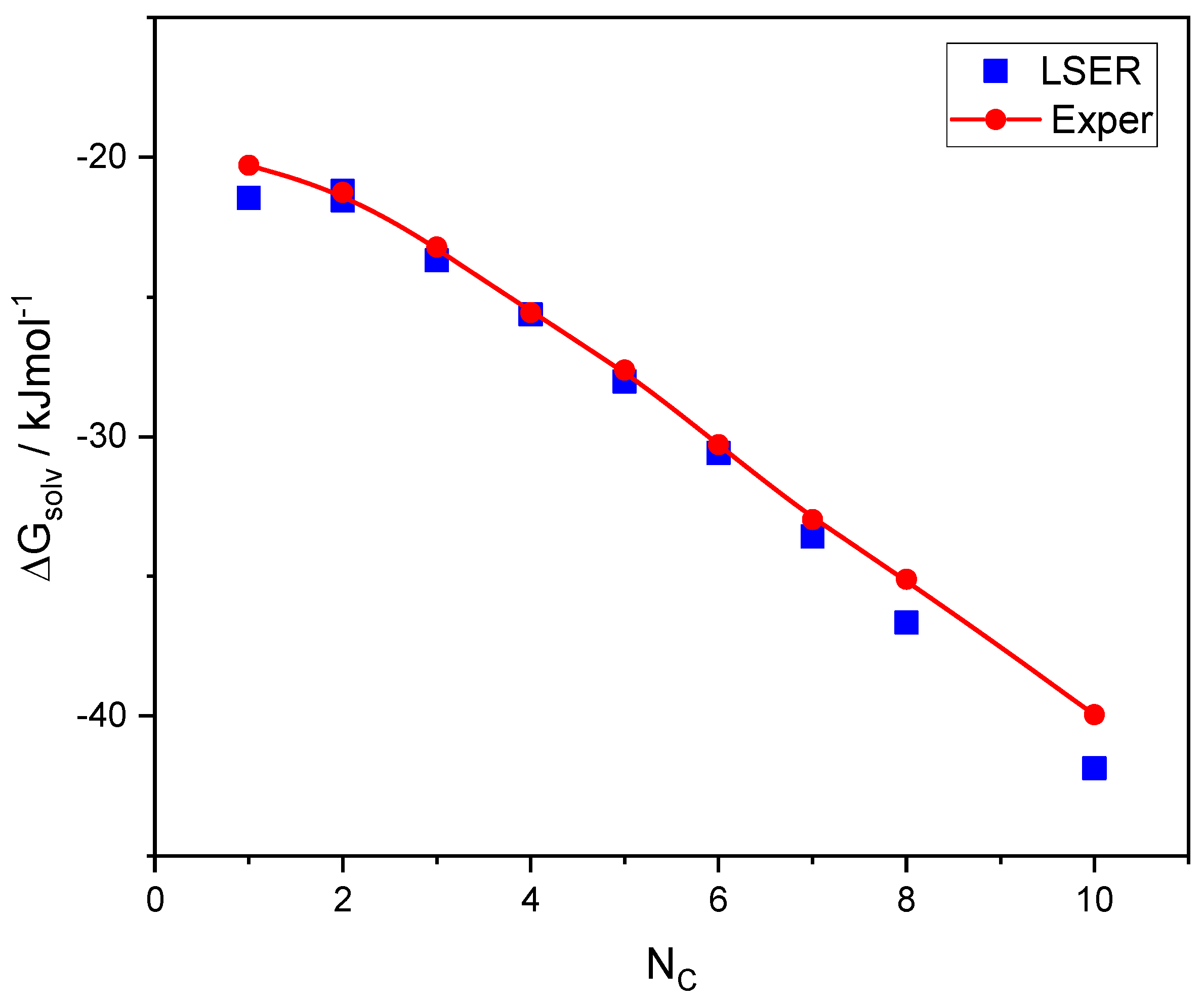
A class of hydrogen-bonded compounds that has been extensively studied in the literature is alkanols. Both LSER descriptors and LFER coefficients are available for this class [16,60], and are summarized in the Supplementary Materials (SM). Thus, we may compare the LSER predictions of solvation free energy with corresponding experimental data [49], the results of which are shown in Figure 2.

As shown in Figure 2, there is a good agreement between the LSER predictions of solvation free energies and the experimental results. This is, then, directly exchangeable thermodynamic information. Only the experimental data [49] obtained at 298.15 K are shown in Figure 2. However, data on enthalpies and entropies of self-solvation of 1-alkanols at various temperatures are also known [49], which can be converted to the free energies of self-solvation at 298.15 K using the following equation: $\Delta G_{}^S=\Delta H_{}^S-298.15\Delta S_{}^S$. These converted data are reported in Table S5 along with the original temperature, T_or, for which the enthalpy and entropy data are known [49]. As shown in Table S5, the discrepancies in the experimental data regarding the free energies of self-solvation of alkanols are almost always less than 1%.

The constant LFER coefficients, c, are rather negligible for all 1-alkanols [16,60], and each of the product terms is therefore considered to reflect the full corresponding contribution to the solvation free energy. Alkanols are self-associating compounds with a significant hydrogen bonding contribution that deserve particular attention.

The five contributions to the equilibrium constant, −logK^S, for the self-solvation free energy of alkanols, as given by the five products of the linearity Equation (2), are reported in

Table 1. The five contributions (cf. Equation (2)) to the equilibrium constant (−logK^S) for the self-solvation free energy of alkanols [16,60]: the hydrogen bonding contribution, $\Delta G_{hb}^S$, to the solvation free energy (in kJ/mol); the experimental [61] hydrogen bonding contribution, $\Delta H_{hb}^S$, to the self-solvation enthalpy (in kJ/mol); and the calculated hydrogen bonding contribution to the self-solvation entropy (in J/mol K) of alkanols.

Alkanol	eE	sS	aA	bB	lL	$\mathbf{\Delta }{\mathit{G}}_{\mathit{h}\mathit{b}}^{\mathit{S}}$	$\mathbf{\Delta }{\mathit{H}}_{\mathit{h}\mathit{b}}^{\mathit{S}}$	$\mathbf{\Delta }{\mathit{S}}_{\mathit{h}\mathit{b}}^{\mathit{S}}$
METHANOL	0.095	0.578	1.645	0.656	0.747	−13.14	−15.1	−6.58
ETHANOL	0.058	0.363	1.441	0.572	1.265	−11.49	−16.9	−18.14
1-PROPANOL	0.056	0.314	1.439	0.516	1.784	−11.16	−17.7	−21.93
1-BUTANOL	0.063	0.323	1.365	0.424	2.312	−10.21	−17.7	−25.11
1-PENTANOL	0.035	0.225	1.392	0.463	2.793	−10.59	−17.7	−23.85
1-HEXANOL	0.043	0.245	1.330	0.432	3.294	−10.06	−17.7	−25.62
1-HEPTANOL	0.045	0.234	1.323	0.388	3.837	−9.77	−17.7	−26.61
1-OCTANOL	0.043	0.236	1.283	0.364	4.349	−9.40	−17.7	−27.84
1-DECANOL	0.017	0.150	1.292	0.354	5.382	−9.40	−17.7	−27.84
2-PROPANOL	0.068	0.261	1.237	0.591	1.571	−10.43	−17.3	−23.03
2-PENTANOL	0.065	0.182	1.237	0.573	2.650	−10.34	−17.3	−23.36

. As shown, excluding cavitation contribution (lL), the main charge contribution to solvation free energy is hydrogen bonding. As observed in columns 4 and 5, the acid–base contribution, aA, is significantly different from the base–acid interaction, bB, for all alkanols. The difference (log) is 0.93 ± 0.06 for 1-alkanols and 0.65 for 2-alkanols. At present, there is no explanation for this difference. Thus, this hydrogen bonding information is not directly transferable at present.

The overall hydrogen bonding contribution, $\Delta G_{hb}^S$, to the self-solvation free energy (calculated as $\Delta G_{hb}^S$ = −2.303 × RT × (aA + bB)) is shown in column 7 of Table 1. In column 8, the estimated hydrogen bonding contribution to self-solvation enthalpy determined on the basis of experimental spectroscopic measurements and a set of assumptions regarding the separation of the hydrogen bonding contribution from the rest of the contributions to self-solvation enthalpy [61]. The reported values (on the order of −17 kJ/mol) are in rather considerable disagreement with the widely accepted values reported in the literature (on the order of −25 kJ/mol) [62,63,64]. In column 9 of the table, the hydrogen bonding entropy change with self-solvation is reported. In contrast to enthalpy, the values reported for this change in entropy are in rather good agreement with the widely accepted values (on the order of −25 J/K mol), with the exception of methanol and ethanol [54,62,63,64].

The key point from the above exposition is that, even for the extensively studied alkanols, there are notorious discrepancies in the open literature regarding hydrogen bonding contribution. Since hydrogen bonding contributions constitute the main charge contributions to the solvation free energies of these systems, it would be useful to see what the above thermodynamic framework and analysis tell us.

First of all, although often minor, a distinction should be made between hydrogen bonding solvation free energy, $\Delta G_{hb}^S$, and free energy change upon the formation of the hydrogen bond, $\Delta G_{ij}^{hb}$, as well as for the corresponding hydrogen bonding enthalpies. The latter quantity characterizes the average strength of a specific interaction, and is well suited to carrying out modeling using explicit equations, like Equations (31) or (41). This quantity, when used in a consistent thermodynamic framework, should lead to expressions (like the above terms, F_ij) for the former quantity, $\Delta G_{hb}^S$, which is part of the measurable overall solvation free energy. The same holds true for the corresponding enthalpies, although the difference in enthalpies is significantly reduced. As an example, in the case of self-solvation, we may start from the simple Equation (32) and examine the above differences.

If the logarithm of F_ij in Equation (30) or (32) were written without the constant term, as in the LSER model, this would imply than lnF₁₂ = −$\Delta G_{ij}^{hb}/2RT$(cf. Equation (31)) and the hydrogen bonding equilibrium constant, K₁₂, were identical to the hydrogen bonding component of the solvation equilibrium constant, K^S, as well as, of course, with F₁₂. This would simplify things, and the differences described above would be zero. The correction constant to F₁₂, however, implies that the two Ks are conceived differently by the two modeling approaches. Thus, the LSER quantity, −2.303RT(A₁a₂ + B₁b₂) = $\Delta G_{hb}^S$, cannot be considered identical to $\Delta G_{12}^{hb}$. The way hydrogen bonding contributes to the solvation free energy depends on the nature and multiplicity of the interacting sites, and this requires some corresponding correction to the plain sum of the LFER products, A₁a₂ + B₁b₂. Neither should F₁₂ be considered to be identical to K₁₂. Similar concerns apply to all models based on divisions of intermolecular interactions.

By combining Equation (19) with Equation (28) or with Equation (29), we obtain the following equation (the subscript 1 in Equation (49) should be taken as corresponding to the acid site, while the subscript 2 corresponds to the base site):

$$\begin{array}{l}\Delta H_{hb}^S=\Delta H_{hb,12}^S+\Delta H_{hb,21}^S=-2R{T}^2{\left(\frac{\partial \left(\Delta G_{hb,12}^S/RT\right)}{\partial T}\right)}_P=-2R{T}^2{\left(\frac{\partial \ln (F_{12})}{\partial T}\right)}_P\\ =-2R{T}^2{\left(\frac{\partial \ln \left(\left(1+2\sqrt{K}\right)/\left(1+\sqrt{5}\right)\right)}{\partial T}\right)}_P=-2R{T}^2{\left(\frac{\partial \ln \left(1+2\sqrt{K}\right)}{\partial T}\right)}_P\\ =-2\frac{R{T}^2}{1+2\sqrt{K}}\frac{K}{\sqrt{K}}\frac{\partial }{\partial T}{\left(\frac{\Delta H_{12}^{hb}-T\Delta S_{12}^{hb}}{RT}\right)}_P=\frac{2K}{\sqrt{K}+2K}\Delta H_{12}^{hb}\\ \end{array}$$

(49)

Thus, at values of K that are not very low, the hydrogen bonding solvation enthalpy may be considered to be close to the corresponding change in enthalpy upon the formation of the acid–base hydrogen bond. In alkanols in which K is greater than 350, their difference is less than 2%. Thus, information on this quantity would essentially be directly transferable. As a consequence, the enthalpy described in column 8 of Table 1 should have been nearly identical to the change in enthalpy $\Delta H_{12}^{hb}$, which is not the case. This discrepancy highlights the problem caused by the lack of consensus in the literature on the strength of hydrogen-bonding interactions in alkanols. However, the PSP approach and the equation-of-state model permit the estimation of this change in enthalpy on the basis of other thermodynamic properties, as well.

The free energy and enthalpy data presented in Table 1 were used to correlate the basic thermodynamic quantities of alkanols (vapor pressure, vaporization heat, density, and solubility parameters) [65] with those of the LFHB and the more advanced NRHB [52,53,54,57,58] equation-of-state models. The LFHB scaling constants with which the best correlations were obtained are reported in the SM. In

Table 2. The scaling constants and the hydrogen bonding solubility parameters of alkanols.

Solvent	ε*/ J mol−1	ε*s/JK 1 mol−1	v*sp0/cm3 mol−1	v*sp1/ × 104	$\mathbf{\Delta }{\mathit{H}}_{22}^{\mathit{h}\mathit{b}}$/ kJ mol−1	ΔSh22/ JK−1 mol−1	$\mathbf{\Delta }{\mathit{G}}_{22}^{\mathit{h}\mathit{b}}$/ kJ mol−1
METHANOL 1	4609	−0.117	1.165	2.5	−23.60	−28.0	−15.25
METHANOL	4162	1.185	1.131	2	−26.00	−29.5	−17.21
ETHANOL	4134	−0.107	1.128	0	−24.05	−27.5	−15.85
1-PROPANOL	4072	0.330	1.103	−1	−23.60	−26.5	−15.70
1-BUTANOL	4092	0.610	1.097	−1	−23.40	−26.5	−15.50
1-PENTANOL	4076	0.914	1.088	−1	−23.38	−27.0	−15.33
1-HEXANOL	4058	1.090	1.079	−1	−23.08	−26.5	−15.18
1-HEPTANOL	4117	0.730	1.081	−1	−23.10	−27.0	−15.05
1-OCTANOL	4086	1.004	1.075	−1	−23.10	−27.5	−15.18
1-DECANOL	4095	1.311	1.072	−3	−23.10	−28.5	−15.05
ISOPROPANOL	3777	0.267	1.103	−1	−23.50	−26.5	−14.90
2-PENTANOL	3784	0.949	1.072	−2	−23.50	−26.5	−14.75

¹ Scaling constants for methanol accounting for δ_hb [24].

, the LFHB scaling constants are reported, along with the more widely accepted hydrogen bonding enthalpies and entropies [50,51,52,53,54,56,57,58,62,63,64] that were used to obtain the best correlations for the very same set of thermodynamic quantities of alkanols [65]. Two sets of scaling constants are reported for methanol, just to show how sensitive the scaling constants are to the adopted hydrogen bonding parameters.

In

Table 3. The experimental and calculated total solubility parameters and hydrogen bonding solubility parameters of alkanols. LSER and PSP calculations were performed using the hydrogen bonding parameters presented in Table 1 and Table 2, respectively.

Solvent	δt/MPa0.5			δhb/MPa0.5
	LSER calc	σ	Exp [61]	LSER calc	σhb	Exp [24]
METHANOL 1	27.8	30.2	29.4	17.9	22.8	22.3
METHANOL	27.8	30.4	29.4	17.9	24.4	22.3
ETHANOL	25.0	26.3	26.2	14.9	19.3	19.4
1-PROPANOL	23.8	24.3	24.6	13.3	16.9	17.4
1-BUTANOL	22.8	23.1	23.5	11.5	14.9	15.8
1-PENTANOL	21.9	22.6	22.4	10.5	13.6	13.9
1-HEXANOL	21.3	21.9	22.1	9.4	12.5	12.5
1-HEPTANOL	21.0	21.7	21.8	8.6	11.7	11.7
1-OCTANOL	20.5	21.0	21.0	8.6	11.0	11.9
1-DECANOL	20.1	20.4	20.2	7.0	9.8	10.0
ISOPROPANOL	22.8	23.6	23.8	12.6	16.4	16.4
2-PENTANOL	21.1	21.8	21.8	10.2	13.6	13.3

¹ With scaling constants for methanol best accounting for δ_hb [24].

, the calculated solubility parameters are compared with the two sets of hydrogen bonding parameters described in Table 1 and Table 2, as well as with literature data. It can be observed that the hydrogen bonding data in Table 1 do not seem to be compatible with the experimental data regarding total solubility parameters, especially in the case of the lower (MW) alkanols, or with the Hansen solubility parameters for hydrogen bonding [24]. In fact, the large discrepancies for the later may be an explanation for the discrepancies in the former. The discrepancies were somewhat larger, when using the NRHB [57,58], rather than the LFHB, model. As shown by Equation (40), the change in enthalpy, $\Delta H_{12}^{hb}$, strongly affects, in a direct manner, the hydrogen-bonding PSP and thus the corresponding solubility parameter, δ_hb. Thus, the correlation of this parameter can be considered to be a direct test of the accuracy of the proposed $\Delta H_{12}^{hb}$ values. It seems that the hydrogen bonding parameters reported in Table 1, which have apparently been adopted by the LSER model [40], are not compatible with the corresponding solubility parameter data described in the literature [24,61].

So far, we have essentially confined ourselves to the self-solvation of alkanols. We could further test the accuracy of the proposed hydrogen bonding energies by looking at the solvation of various solutes in alkanol solvents. In this way, we could extract useful conclusions, especially from solutes that form hydrogen bonds with alkanols. In essence, if the true values of hydrogen bonding free energy and enthalpy of alkanols are significantly more negative than what is estimated by the LSER model, then, in the solvation free energies of various solutes in alkanol solvents, this would show up in the LSER model estimations by being somewhat less negative than the corresponding experimental values.

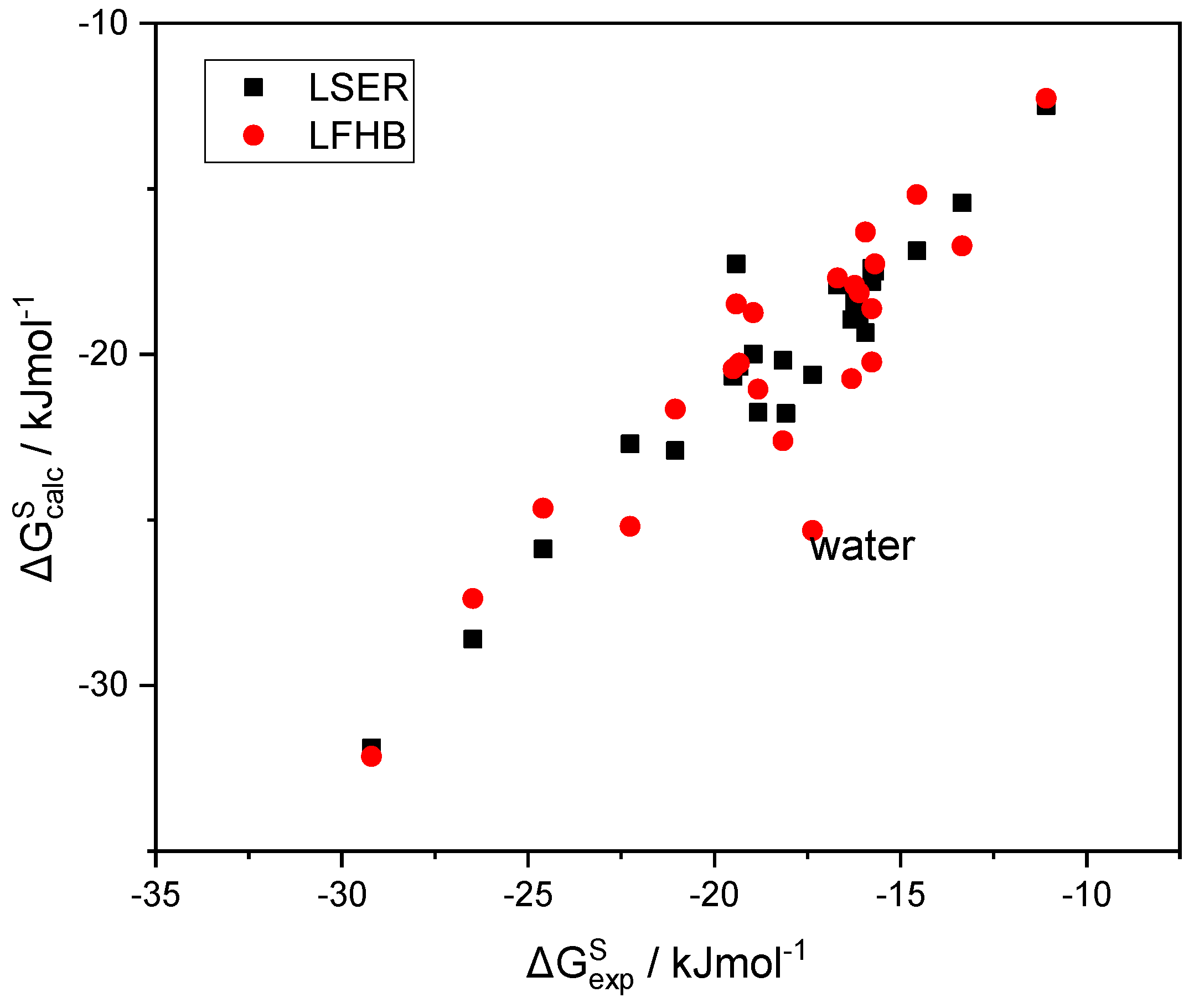
In Figure 3, the LSER estimations of the solvation free energy of a variety of solutes in 1-octanol are plotted as a function of the corresponding experimental data [49]. In the same figure, alternative predictions are also reported in which the LSER hydrogen bonding contribution to $\Delta G_{12}^{hb}$ (Table 1) is replaced with the corresponding LFHB contributions with the above, more widely used, hydrogen bonding parameters (Table 2). It can be seen that the two sets of predictions are practically identical, except for the notable case of water, where the LSER estimation is significantly less negative than the LFHB one, while being in rather good agreement with the experimental results. This picture is nearly the same for the solvation in all alkanols as solvents. Detailed tables with the data reported in Figure 3 are provided in the Supplementary Materials (SM).

As can be observed in Figure 3, the scatter of the experimental solvation free energies [49] does not permit clear judgement regarding the accuracy of the alternative sets of hydrogen bonding parameters used. The outlier in the LFHB correlation (water) is quite interesting, and will be extensively discussed in a forthcoming paper dedicated exclusively to water and aqueous systems.

All of the above indicate that the LSER estimations of hydrogen bonding contribution to solvation free energies in alkanols raise several questions, and should probably be reconsidered. However, if they were to be reconsidered, their reconsideration might affect the other products of the LFER linearity Equations (1) and (2), and such structural changes in the LSER database are not easy to make. In fact, the accuracy of the experimental results for overall solvation free energies may not always be high enough to capture the differences in hydrogen bonding parameters or, probably, the parameters of the other intermolecular interactions. These obstacles are mentioned here, just to indicate the challenges faced by PSP development. If these obstacles could be overcome, the transfer process described above might be reversed, and information from PSPs could be used to enhance the LSER database.

Assuming that the values of σ_a and σ_b are known from other sources, say, from the COSMO-RS model [35,36,37,38,39] or from molecular dynamics simulations, Equation (47) can be used to calculate the hydrogen bonding LSER molecular descriptors. This particular transfer, either from LSER to PSP or from PSP to LSER, is meaningful and useful when the same constant k is used in the equation. This constant may be obtained using Equation (31) if $\Delta G_{ij}^{hb}$ is known. In

Table 4. The acidity and basicity LSER descriptors, A and B [16], the free energy change upon self-association, $\Delta G_{ij}^{hb}$, the corresponding kRT product, and the readjusted A’ and B’ descriptors to be used with a universal value of kRT = 84 kJ/mol.

Solvent	A	B	$-\mathbf{\Delta }{\mathit{G}}_{\mathit{i}\mathit{j}}^{\mathit{h}\mathit{b}}$/ kJ mol−1	−kRT/ kJ mol−1	A’	B’
METHANOL	0.43	0.47	17.21	85.13	0.433	0.473
ETHANOL	0.37	0.48	15.85	89.25	0.381	0.495
1-PROPANOL	0.37	0.48	15.70	88.40	0.380	0.492
1-BUTANOL	0.37	0.48	15.50	87.26	0.376	0.491
1-PENTANOL	0.37	0.48	15.33	86.31	0.374	0.489
1-HEXANOL	0.37	0.49	15.18	85.15	0.370	0.489
1-HEPTANOL	0.37	0.48	15.05	84.73	0.369	0.485
1-OCTANOL	0.37	0.49	14.90	83.89	0.365	0.485
1-NONANOL	0.37	0.49	14.75	81.82	0.362	0.484
1-DECANOL	0.36	0.49	14.60	82.29	0.361	0.482
ISOPROPANOL	0.31	0.56	15.90	92.65	0.322	0.588
2-PENTANOL	0.33	0.56	15.60	85.38	0.329	0.565

, the estimations of this constant are reported for alkanols based on the hydrogen bonding parameters, $\Delta G_{ij}^{hb}$, presented in the table. It can be seen that k is nearly constant. In fact, on the basis of analogous calculations performed for other solute–solvent systems, including aqueous ones, it seems that the values of k center around k = 33.9 or kR × 298.15 = 84,000 J/mol. The adoption of such a universal value for the constant k would greatly augment the predictive capacity of LSER and PSP, as well as other interconnected QSPR-type databases. However, the prerequisite for this remains the agreement on the values of $\Delta G_{12}^{hb}$ or $\Delta H_{12}^{hb}$ for several hydrogen-bonded compounds. In fact, the adoption of such a universal value for k would also require a rather minor change in the A and B LSER descriptors to A’ and B’, as reported in Table 4, in order to obtain the same solvation free energy as the product kRTA’B’.

Having agreed on the hydrogen bonding parameters, an agreement on the contribution of hydrogen bonding to the solvation free energy is then feasible. Once this is done, the exchange of information can be continued with the other descriptors. The contribution of non-hydrogen-bonding interactions to PSPs can easily be obtained from the equation-of-state scaling constants. Combining Equations (36)–(39), we get:

$${\sigma }_d^2+{\sigma }_p^2=\tilde{\rho }\frac{E_d^{*}+E_p^{*}}{V_m}=\tilde{\rho }\frac{E_{}^{*}}{V_m}$$

(50)

The dispersive PSP, σ_d, is mainly connected to the McGowan volume, V_x, and, to a lesser extent, to the excess refractivity descriptor, E (cf. Equation (36)). Both V_x and E are rather clearly defined, and practically speaking, Equation (36) is always considered to be valid. Since the total solubility parameter is very often known with good accuracy, Equation (42) permits the estimation of the polar PSP, σ_p, or, equivalently, the LSER polarity descriptor, S, or the interaction energy, E_d*. The polarity descriptor S is not as clearly defined as V_x and E. Thus, the above transfer of information from σ_p may be useful for verification or for a better estimation of S.

4. Discussion

There is no doubt that the LSER approach and database [1,2,3,4,5,6,7,8,9,10,11,12,13,14,15,16,17,18] are very rich in thermodynamic content. For decades, now, the scientific community has used them in numerous applications, with remarkable success. However, the question remains as to how this content might be extracted and transferred for more extensive or specific advanced thermodynamic calculations. In response to this question, an attempt was made in the previous two sections to address some challenging issues related to the interconnection between the LSER approach and database [1,2,3,4,5,6,7,8,9,10,11,12,13,14,15,16,17,18] and the equation-of-state approach and Partial Solvation Parameters [26,27,28,29,30,31,32,33,34].

The three LSER molecular descriptors, V$x$, E, and L, are rather clearly defined. The remaining three descriptors for the polar and strong specific interactions, S, A and B, are not as clearly defined and, to a great extent, their determination has been performed through regression and fitting to experimental data. In this regard, the more specific question is: how can hydrogen bonding or strong (Lewis) acid–base interactions, reflected by the descriptors A and B, be separated from the remaining weaker polar interactions, reflected by the descriptor S? Furthermore, the even more specific question is: on what scale is acidity or basicity expressed? This concept of “scale” is needed whenever aiming to perform a quantitative comparison of similar properties or entities.

In the previous two sections, the focus was primarily on descriptors A and B, and indirectly on descriptor S. The basis of the discussion was the very fact that thermodynamic quantities such as solvation free energy can be estimated successfully using a simple linear equation (Equation (2)). The obvious first step was to examine the thermodynamic basis of this very linearity, especially for the hydrogen bonding contribution. The tool used for this examination was a simple statistical thermodynamic model, able to handle simple as well as complex hydrogen-bonding interactions, including intramolecular interactions, cooperativities and three-dimensional networks [50,51,52,53,54,55,56,57,58]. The minimal features of the model were used here, since the bulk of hydrogen-bonded solutes and solvents are attributed one donor and/or one acceptor site when using the LSER approach, while densities or external pressures are not explicitly taken into account. Even when considering temperature variations, the bulk of the data are reported at a temperature of 25 °C. Thus, hydrogen-bonding interactions could be handled as simple quasi-chemical reactions with a free energy change upon formation and an equilibrium constant. For reader convenience, a step-by-step derivation of the key equations with the corresponding assumptions is provided in the SM, along with the implementation of the central simple assumption for this (hydrogen bond) free energy change upon formation, namely, $\Delta G_{12}^{hb}$ = −kA₁B₂.

With this exercise, it was verified that the hydrogen bonding contribution to solvation free energy may indeed be expressed in a linear-like manner similar to the LSER, as shown in Equation (2). This similarity is gratifying, but more interesting is the insight contained in the new equations. In the main text, above, the case of molecules with one donor and/or one acceptor was presented. The case of molecules with two donors and/or two acceptors is presented in the Supplementary Materials (SM). The acid (1)–base (2) contribution to solvation free energy is given by the following general equation:

$$\ln \left(F_{12}-\lambda \right)=A_1\left(k{B}_2\right)+c_2^{\prime }=A_1{a}_2^{\prime }+c_2^{\prime }$$

(51)

and the base(1)–acid(2) contribution by the following symmetric equation:

$$\ln \left(F_{21}-\lambda \right)=B_1\left(k{A}_2\right)+c_2^{\prime }=B_1{b}_2^{\prime }+c_2^{\prime }$$

(52)

The constant c₂^′ is an exclusive property of the solvent (component 2). The constant λ reflects the character of the hydrogen-bonding interaction. In one-donor–one-acceptor solute–solvent systems, λ = $2/\left(1+\sqrt{5}\right)$ and, upon self-solvation, λ = $1/\left(1+\sqrt{5}\right)$. In the case of two-donor–two-acceptor solute–solvent systems, λ = 2/4 and, upon self-solvation, λ = 1/4.

Due to their symmetric character, Equations (50) and (51) indicate that, upon self-solvation, the acid–base and the base–acid contributions are identical, that is, F₁₂ = F₂₁ and A₁a₂′ = B₁b₂′. What is even more interesting, though, is that both solvent coefficients, a₂′ and b₂′, are expressed explicitly by the plain relations, a₂′ = kB₂ and b₂′ = kA₂.

It seems, however, that LSER was developed differently with respect to hydrogen-bonding interactions. Linearity is obeyed, but upon self-solvation, A₁a₂ is different from B₁b₂. Apparently, one or both of these products also contains the information of constant c₂′. The constant λ does not show up when using the LSER approach, since it handles solute–solvent interactions exclusively as a one-donor–one-acceptor interaction. Thus, at present, the extraction of separate information on acidity and basicity contributions is not quite straightforward. If this were possible, this information could be transferred to the corresponding PSPs via Equations (45) and (46), and practically useful equation-of-state calculations could be performed.

The overall hydrogen bonding LSER contribution seems easier to extract and transfer. Even there, however, much care must be exercised. In the previous section, the example of alkanol solvents was discussed, where the value of enthalpy-change upon the formation of OH–OH hydrogen bonds is still controversial today. The value adopted by LSER (on the order of −17 kJ/mol) is rather drastically different from the more widely adopted value (on the order of −25 kJ/mol), and this by itself remains a challenging issue in the literature.

If the above issues were clarified, the PSP approach could facilitate the determination of the descriptor S once the hydrogen bonding contribution was known. As shown in the previous section, the solubility parameter, and especially its hydrogen bonding component, are sensitive to the value of the hydrogen bonding enthalpy. The overall solubility parameter is a rather well-defined (and measurable) quantity. Thus, once the hydrogen bonding contribution is known, it may be relatively easier to separate the remaining dispersion and polar contributions.

It should be stressed, once again, that the above analysis is not a criticism of any database or polarity scale reported in the literature. It is just an attempt to develop a thermodynamic basis for the safe exchange of information between different databases. The interconnection between LSER and PSP is just an example used to discuss some problems associated with this effort. The above discussion was not exhaustive, by any means, with respect to these problems, but their nature and key aspects have hopefully been exposed.

The calculations in the present work were confined to systems of alkanols. Water and aqueous systems will be discussed in a forthcoming manuscript. Systems of glycols will also be discussed separately, since they possess two distant donor sites and two acceptor sites in their molecules (cf. SM file). Heterosolvated compounds, possessing one type of hydrogen bonding site only—donor or acceptor—are also a separate class of compound, and will be discussed after self-associating or homosolvated compounds. These studies will contribute to our understanding of the thermodynamic content of the LSER linearity terms and the factors affecting them.

It should be stressed that the purpose of this manuscript was not to report a full new database in place of the current LSER database. The development of such a full database is not an easy task, and would require a concerted effort and wider collaboration. In this series of papers, we discuss various classes of compounds (e.g., alkanols, water and aqueous systems, heterosolvated compounds, etc.), but we are far from establishing a full database. We hope that this manuscript will stir broader interest and promote the concerted effort and collaboration required.

In summary of the key messages of this work, the LSER model with its database is not only a valuable predictive tool that is rich in thermodynamic information, the linearity of LFER indeed has a sound thermodynamic basis. It seems, however, that this thermodynamic basis was either not known, or it was disregarded, and the development of the LSER database was carried out on a more or less empirical basis using plain linear regressions and correlations of experimental data, with little interest in the thermodynamic consistency of the reported LFER parameters. As an example of this inconsistency, the acid–base interaction, aA, is often drastically different from the very same base–acid interaction, bB, upon self-solvation. This makes it difficult to extract thermodynamic information from the LSER database in its current form, in spite its remarkable potential. There is no need whatsoever to change LSER descriptors and LFER parameters for current applications of the LSER database. However, since there is now an explicitly known thermodynamic basis, the LSER database could be restructured or redesigned on this basis, if there is an interest in the exchange of thermodynamic information. With a firm thermodynamic basis, it would be meaningful to exchange information on thermodynamic quantities among a number of different databases.

5. Conclusions

The LSER model and database, which is very useful in numerous applications, are also very rich in thermodynamic information, and some key problems associated with the extraction and transfer of this information were discussed in this work. A thermodynamic basis for the linearity of the LFER/LSER approach was proposed and used to provide an interconnection between the LSER molecular descriptors and the corresponding Partial Solvation Parameters (PSPs). It was shown that, in contrast to the well-defined thermodynamic quantities, much care must be exercised when transferring information based on the divisions of intermolecular interactions, since they necessarily have an inherently varying degree of arbitrariness. The LSER database has not been developed, to date, on the above thermodynamic basis, and some aspects of its departure from this were discussed, in an effort to recover thermodynamic information from the reported molecular descriptors and LFER coefficients. The advantages of adopting this thermodynamic basis were also indicated. This adoption is not a trivial task, and will require a concerted effort by experts in the field. It is hoped that this work will stir sufficient interest in the relevant literature, in this regard.