A Waypoint-Based Flow Capture Location Model for Siting Facilities on Transportation Networks

Abstract

We introduce a waypoint-based flow capture location model (WbFCLM) for siting facilities on networks with the objective of maximally capturing flows. The advantages of the waypoint-based formulation are that (1) demand is modeled along observed trajectories rather than assumed travel paths, and (2) demand is allowed to vary across geographic space. We demonstrate the WbFCLM using a test dataset derived from vehicle tracking data. Though solving the WbFCLM can require considerable computing power, it can be used to site facilities on networks where both flows and demand vary spatially.

1. Introduction

Spatial optimization models are routinely used in transportation geography to configure facilities and allocate their demand along networks [1,2]. The flow capture location model (FCLM) is a classic spatial optimization problem that maximizes the amount of flow captured on a network by sited facilities [3]. In the FCLM, origin–destination (O-D) pairs represent the demand flows, and all nodes are considered potential facilities. The objective function seeks to maximize the flow covered by a user-specified number of facilities [4]. The FCLM is designed to select facility locations that intercept the most network flows based on pre-defined travel paths. These travel paths are typically assumed to be the shortest or fastest route between each O-D pair. Facilities are considered to either fully capture or not capture flow depending on whether they lie on the assumed path. This results in a binary capture structure: if a facility is on the path, all flow between that O-D pair is considered captured; if not, none of the flow is captured. Accordingly, FCLM solutions generally prioritize high-volume corridors because these locations intersect the most assumed paths and maximize flow coverage. The FCLM and its variants are widely used to cite electric vehicle recharging stations [5,6], alternative-fuel refueling locations [7,8], manufacturing facilities [9], park-and-ride lots [10], and related services in transportation networks [11].

Though the FCLM’s binary capture rule is computationally efficient, the model’s applicability is limited by two critical assumptions. First, the model assumes that travelers consistently follow the shortest or fastest path between their origins and destinations [12]. However, substantial empirical evidence shows that route selection is often influenced by factors such as congestion, perceived safety, familiarity, and individual preferences [13,14,15]. As a result, facility siting decisions based on shortest-path assumptions may not align with real-world travel behavior [16], potentially leading to suboptimal facility placements [17]. Second, demand is generally assumed to be uniformly distributed along the selected path. However, in practice, demand often varies across geographic space and may concentrate at specific locations, such as intersections, bottlenecks, or popular destinations [18]. Uniform demand assumptions can cause facilities to be sited in locations that capture high flow volumes but miss key areas of concentrated demand where facility placement would be most beneficial [19,20]. Some strategies to improve the traditional FCLM have been proposed, such as those that include stochastic flows [21,22], facility hierarchies [23], and measures of facility capacities [24]. However, there is still a need for more robust flow capture problems that can account for spatial variability in both travel paths and demand.

Recent studies have demonstrated the potential of trajectory-based analyses to better reflect actual travel patterns [25]. These approaches use GPS-based trajectory data to identify where travelers actually move through a network, rather than relying on assumed O-D paths. However, most existing applications focus on descriptive analyses or route choice modeling and rarely integrate trajectory data directly into facility optimization problems. Incorporating waypoint-level demand and observed trajectories into flow capture models remains uncommon, in part due to the computational challenges associated with processing large datasets and modeling distance-decay effects [26]. Traditional FCLMs do not scale well to this level of granularity because of their reliance on O-D pairs, potentially limiting their usefulness in modern, data-rich transportation systems.

Accordingly, we introduce the waypoint-based flow capture location model (WbFCLM) as an alternative spatial optimization problem for siting facilities on networks. Like the traditional FCLM, the objective of the WbFCLM is to maximize the coverage of flows on a network. However, the WbFCLM is formulated using waypoints from trajectories of tracking data instead of assumed O-D paths. There are two potential advantages to using a waypoint-based formulation. First, demand is modeled along observed trajectories rather than assumed travel paths, enabling a more accurate representation of flows across a network and potential demand points. Additionally, the use of waypoints allows demand to vary spatially, as demand can be assigned to each waypoint in a trajectory rather than assigning a single measure to each O-D pair. By assigning demand to each waypoint, the WbFCLM can model the partial capture of flows using distance-decay functions, recording both how much demand is covered and where it is covered. In this paper, we first present the WbFCLM formulation. Second, we test the performance of the WbFCLM using a test dataset derived from real-world spatial data. Finally, we discuss the strengths and limitations of applying the WbFCLM to practical problems.

2. Waypoint-Based Flow Capture Location Model

Here, we introduce the WbFCLM for optimally siting facilities on a network with the objective of maximizing the capture of observed flows with varying demand. Though the WbFCLM shares the goal of maximizing flow capture with traditional FLCMs, it is formulated in a similar way to the maximal covering location problem (MCLP) in how it defines capture, or coverage [27,28]. Specifically, flows and demand are represented by waypoints along individual trajectories between origins and destinations in a network. Potential facility locations occur at points along a network; these can be either waypoints from the trajectories or any other nodes on a network. Decay effects can be modeled for the facilities, where their effectiveness declines as a trajectory moves further away. The WbFCLM can be formulated as a linear optimization problem using the following notation:

Objective

$$Maximize Z=\sum _{i\in I}\sum _{k\in K_i}\sum _{j\in J}{X}_{ikj }$$

(1)

subject to

$$\sum _{j\in J}{X}_{ikj}\le r_k; \forall i\in I, \forall k\in K_i$$

(2)

$$X_{ikj}-w_{ikj}{r}_{ikj}{Y}_j\le 0; \forall i\in I,\mathrm{for} k \mathrm{located} \mathrm{at} j \mathrm{and} l \ge k$$

(3)

$$\sum _{j\in J}{Y}_j=p$$

(4)

$$0\le X_{qkj}\le r_k;\forall q\in Q, \forall k\in K_i, \forall j\in J$$

(5)

$$Y_j\in \left(\mathrm{0,1}\right); \forall j\in J$$

(6)

where

• $I=\left\{1, \dots ,i,\dots , m\right\} \mathrm{denotes} \mathrm{the} \mathrm{set} \mathrm{of} m \mathrm{total} \mathrm{trips} i \mathrm{that} \mathrm{cross} \mathrm{the} \mathrm{study} \mathrm{area}$;
• $K_i=\left\{1,\dots ,k,\dots ,l,\dots n\right\} \mathrm{denotes} \mathrm{the} \mathrm{set} \mathrm{of} n \mathrm{waypoints} \mathrm{in} \mathrm{trip} i,$
• $\mathrm{where} \mathrm{waypoint} l \mathrm{is} \mathrm{located} \mathrm{after} k$;
• $J=\left\{1, \dots , j,\dots ,s\right\} \mathrm{denotes} \mathrm{the} \mathrm{set} \mathrm{of} s \mathrm{potential} \mathrm{facility} \mathrm{locations} j$;
• $p=\mathrm{specified} \mathrm{number} \mathrm{of} \mathrm{facilities} \mathrm{to} \mathrm{locate}$;
• $r_k=\mathrm{demand} \mathrm{at} \mathrm{waypoint} k$;
• $w_{ikj}=\mathrm{decay} \mathrm{in} \mathrm{demand} \mathrm{coverage} \mathrm{for} \mathrm{waypoint} k \mathrm{in} \mathrm{trip} i \mathrm{for} \mathrm{facility} j$;
• $Y_j=1 \mathrm{if} \mathrm{a} \mathrm{facility} \mathrm{is} \mathrm{located} \mathrm{at} j ;0 \mathrm{otherwise}$;
• $X_{ikj}=\mathrm{amount} \mathrm{of} \mathrm{demand} r \mathrm{covered} \mathrm{at} \mathrm{waypoint} i \mathrm{that} \mathrm{is} \mathrm{covered} \mathrm{by} \mathrm{facility} j$.

The objective function (1) maximizes the demand covered by facility j for waypoint k in trip i. Constraint (2) stipulates that the demand covered for waypoint k in trip i by facility j cannot exceed the demand present at that waypoint. Constraint (3) ensures that the demand potentially covered by facility j for waypoint k in trip i can only be covered if facility j is selected. In other words, facility j can potentially cover demand at waypoint k and waypoint l that follows. The amount of demand potentially covered is determined by multiplying the demand at that waypoint $r_k$ by a decay factor $w_{ikj}$, potentially within a maximum coverage distance. The decay factor could be calculated based on the inverse distance between the facility location and waypoint, or similar methods. Constraint (4) specifies that the number of facilities j selected by the model must be equal to the p number of facilities the user decides to select. Constraint (5) bounds the amount of demand covered by waypoint k in trip i for facility j between zero and the demand at that waypoint. Constraint (6) imposes binary restrictions on Y_j, which determines which facilities j are located by the model. The next section applies the WbFCLM to a test dataset derived from vehicle tracking data.

3. Methods

3.1. Test Data

We developed a test dataset to demonstrate the application of the WbFCLM in a realistic setting. The goal was to construct a hypothetical siting problem using real-world geospatial features, observed traffic flows, and simulated spatially varying demand to provide a rigorous evaluation of the model’s performance. We derived our test data from an 8.2 km² region encompassing the University of South Florida Tampa campus grounds and its immediate surroundings (Figure 1). The campus is located at approximately 28.06° N, 82.4° W in the City of Tampa within Hillsborough County, Florida. Average Annual Daily Traffic (AADT) volumes at mileposts along major road segments in the study area were 42,735 for Fletcher Avenue in 2017; 5300 for 50th St in 2019; 65,550 for Fowler Ave. in 2017; and 52,277 for Bruce B. Downs Blvd. in 2017 (Florida Department of Transportation). We selected this site because of data availability and our familiarity with the location.

We obtained personal (i.e., non-commercial) vehicle tracking data for Hillsborough County collected during the month of September 2017 from INRIX, Inc., (Kirkland, WA, USA) to serve as the input waypoints for the model. INRIX aggregates anonymous, real-time GPS probe data from a variety of sources, including connected cars, commercial fleets, and mobile devices, with location, time, speed, and heading metadata [29,30]. All data are map-matched to roadway segments using proprietary algorithms, and are continuously collected and quality-checked before being delivered via the INRIX Trip Analytics platform [31].We used a ~10% sample of the county-wide dataset, which, when clipped to the study area, yielded tracking data for 6897 trips from 4247 unique personal vehicles. The data included 88,823 waypoints collected at sampling intervals of 1 min (Figure 1a).

We used the National Transportation Dataset (USGS, 2020) to map approximately 73 km of roadways in the study area. We modeled potential facility locations at approximately 25 m increments along each road segment, with potential facilities located on both the left and right sides of the road (N = 4346). This facility spacing was selected to ensure that facilities could reasonably intercept nearby travel paths while maintaining a manageable number of candidate sites for the optimization process [32].

We modeled demand for facilities on this network by intersecting it with a simulated risk intensity surface generated from vehicle–bicycle collisions in the study area. We obtained collision data for 2012–2020 for the study area from the Florida Department of Transportation (N = 91). We applied kernel density estimation (KDE) to generate a risk surface from the collision locations. KDE is a statistical method that produces a continuous intensity surface representing variation in the density of events by using a kernel function to smooth the pattern of data points [33]. We applied KDE to the collision locations using a bounded Gaussian kernel with a fixed bandwidth of 200 m, as per [34], to generate an intensity surface representing spatially varying demand [35,36] (Figure 1b).

3.2. Application

We applied the WbFCLM to optimally locate facilities to cover demand in the test dataset. The workflow involved three primary stages: the (1) preparation of spatial data, (2) formulation of the optimization model, and (3) solution of the linear program. First, we overlaid the tracking data, potential facility locations, and risk intensity surface in a GIS (ArcGIS v. 10.5, ESRI, Inc., Redlands, CA, USA) to join the relevant spatial information needed to formulate the WbFCLM. Specifically, a single table was generated with a record for each waypoint in the tracking dataset. The table contained the following information: the trip identifier (ID), waypoint ID, ID of the potential facility located on the same 25 m segment as the waypoint, and demand at the waypoint location. This spatial joining step allowed us to efficiently assign each waypoint to its nearest candidate facility and to aggregate demand values in a format compatible with linear programming input.

Second, we developed a custom Python (v. 2.7.1) script to read the table and output the WbFCLM Equations (1)–(6) in linear programming (lp) format. The script was designed to systematically encode the objective function, constraints, and decision variables from the information in the table. The output included a text file listing all equations, complete with variables and equations, for the model in lp format. The generated LP file follows the standard algebraic LP file format, using row-oriented notation for the objective, constraints, variable bounds, and integrality [37].

Third, we attempted to solve the problems using a commercial optimization solver, IBM CPLEX Optimization Studio v. 12.7 (IBM, Inc., Armonk, NY, USA), on a personal computer with an Intel Core i7 processor with 32 GB of RAM. CPLEX was selected due to its robust performance for large-scale mixed-integer programming problems. If optimal solutions were not found within 50,000 s (~14 h) of running time, we re-ran the programs on a computer with increased RAM: an Intel Xeon processor with 128 GB of RAM. The solver was configured to terminate when an optimal solution was found or when the relative optimality gap was reduced below 1%, a commonly accepted convergence criterion in large-scale facility location studies [38].

We ran the WbFCLM under multiple scenarios to explore variability in both solution sets and solution times under different input parameters. Specifically, we ran the model using four quantities of facilities to locate (4, 8, 12, and 16); two distance-weighting kernels (uniform and Epanechnikov) to estimate the decay in facility effectiveness; and five coverage duration values (6, 12, 60, 120, and 240 successive waypoints). We used a uniform kernel to model the scenario where facility effectiveness was binary (either effective or not) for a specified duration, while we used the Epanechnikov kernel to represent a decay from high to low effectiveness over a similar duration. We used numbers of successive waypoints as a measure of coverage duration, as sampling in the dataset was uniform, though distance or travel time could also have been used. We recorded the objective values, selected facility locations, and solution times for each of the scenarios.

4. Results

The lp files for the problem sets ranged from approximately 45 to 600 MB in size, with larger coverage thresholds generating larger sets of equations and file sizes. All scenarios with coverage effectiveness defined as 12, 30, 60, or 120 successive waypoints solved to optimality on the lower-RAM computer. Solution times ranged from approximately 7 to 45,000 s. Scenarios with greater facility quantities and larger coverage thresholds resulted in larger solution times, ceteris paribus. Scenarios using the Epanechnikov kernel to model facility effectiveness also produced longer solution times as compared to those with the uniform kernel. The solver on the computer with the higher RAM found feasible solutions for the 240-waypoint scenarios in less than 36 h with optimality gaps less than 1%.

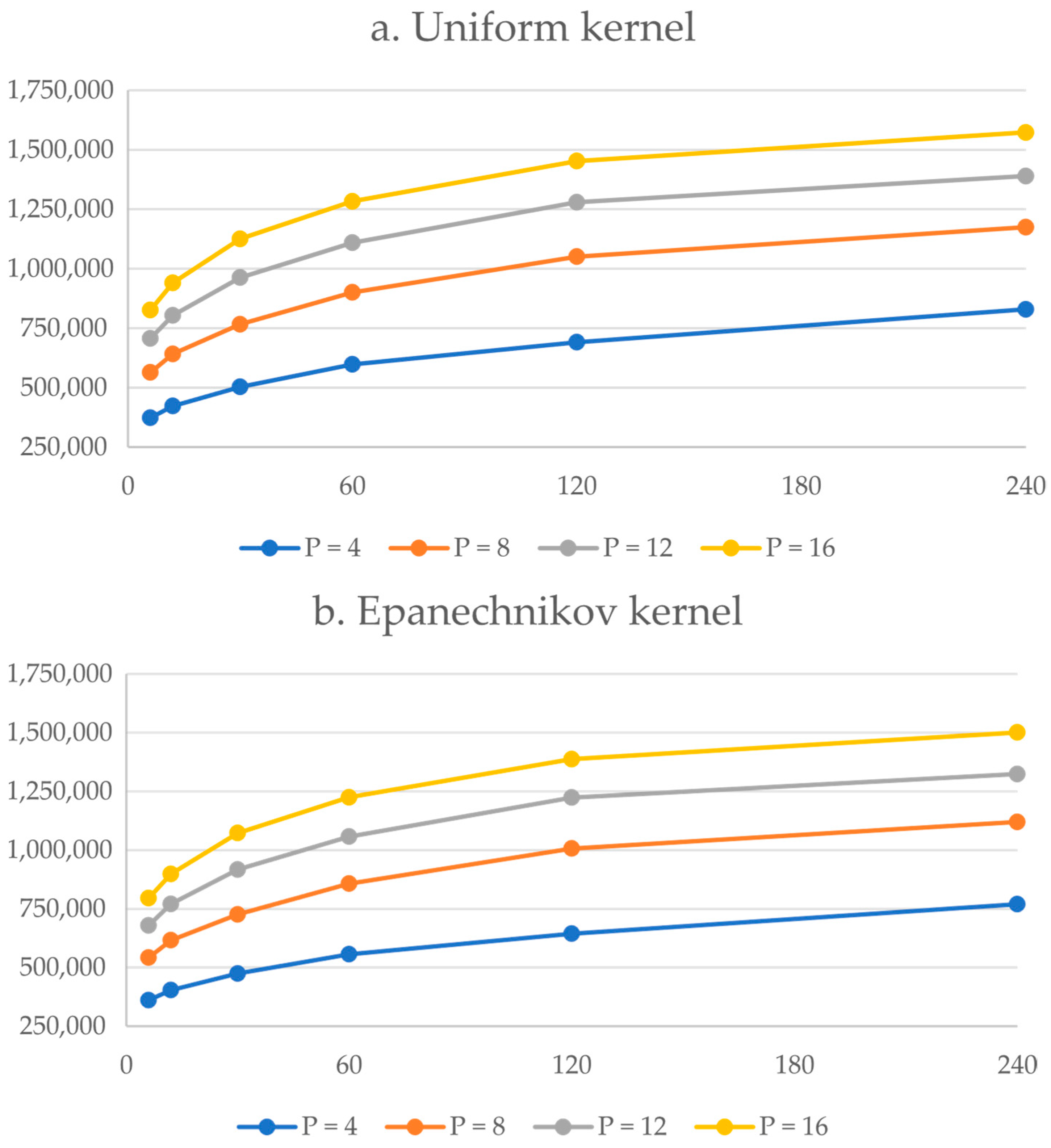
Demand coverage, as measured by the objective value, increased as larger numbers of facilities and effective coverage distances were modeled for both kernels, though the increases were not linear (Figure 2). Coverage increased as additional facilities were added, but gains were relatively larger when the first and second sets of four facilities were added, as compared to the third and fourth. Similarly, extending the coverage effectiveness of facilities increased the objective value for all quantities, but the gains were relatively low when extending coverage beyond 60 waypoints. For both the uniform and Epanechnikov kernels, a four-facility scenario with a coverage effectiveness of 240 waypoints produced a similar objective value to one with 16 facilities with a coverage effectiveness of 6 waypoints. This suggests there is a trade-off between facility quantity and effectiveness.

The selected value for the coverage threshold had the largest impact on optimal facility location. Three facilities were selected preceding the single riskiest intersection (Fowler Ave. and N. 50th St.), along with a fourth preceding a nearby hotspot (Fowler Ave.), in all scenarios (Figure 3a), though the distance away from the hotspot varied slightly depending on the coverage threshold. Smaller thresholds of 6 and 12 successive waypoints resulted in siting facilities immediately approaching collision hotspots in high-traffic areas (Bruce B. Downs Blvd., Fletcher Ave., and Fowler Ave.). Larger thresholds selected locations that captured multiple hot spots along common, longer trajectories. Most scenarios sited facilities in locations along high-traffic intersections bordering campus, although the eight-facility scenario with 240-waypoint coverage and Epanechnikov included one facility location in the interior part of the campus. This location was at the exit for a parking lot that led to multiple hotspots (Figure 3b). Selected facility locations were very similar between the uniform and Epanechnikov kernels for comparable scenarios. For example, solutions for uniform and Epanechnikov problems for four facilities and 12-point coverage both included three of the same facility locations (intersection of Fowler Ave. and N. 50th St.), with the fourth ones selected on the same road segment (Fowler Ave.) but only 50 m apart. This pattern was consistent across similar scenarios.

5. Discussion

We presented the WbFCLM as a variation of a traditional FCLM. Formulated similarly to the MCLP, the advantages of the WbFCLM’s waypoint-based formulation are that it (1) utilizes observed trajectories rather than relying on an OD matrix and assumed shortest paths and (2) models spatially varying demand and facility effectiveness. We demonstrated how the WbFCLM can be solved for problems with moderate volumes of tracking data. Although our test dataset was constructed primarily to evaluate model performance, we anticipate that many real-world problems could benefit from the WbFCLM approach. Examples might include siting traffic safety infrastructure, such as warning signs or wildlife crossings, where unique vehicle paths are critical and risk varies geographically [39]. However, there are several factors that users should consider before applying the WbFCLM to site warning signs or other types of on-network facilities.

First, there are several requirements for formulating the WbFCLM. The WbFCLM requires a representative set of trajectory data for the study area, so data availability and cost can be prohibitive for some applications. Formulating the WbFCLM for big data can also be computationally demanding. As constraint (3) requires linking each waypoint to its nearest potential facility location, a GIS is needed to process the data. The maximum file sizes associated with many GIS software programs may limit the number of waypoints that can be included in an analysis even when data are available (e.g., ~70 million for ArcGIS v. 10.8, ESRI, Inc., Redlands, CA, USA). Furthermore, the generated lp files for the WbFCLM can be large and difficult to solve, even with a commercial solver. Problem size increases with coverage effectiveness, because large values generate additional equations for constraints (3). Although the size of the study area in our application was fairly modest, the largest problems were challenging to solve without high-performance computing resources. Future strategies for solving large problems might include running the problems with high-performance computing, using tracking data with less frequent sampling intervals, reducing the number of potential facility locations, using smaller values for coverage effectiveness, and developing novel algorithms to solve the problems.

Second, formulating the WbFCLM for a given dataset requires consideration of several parameters, including capture effectiveness or decay, and the number of facilities. Though the uniform kernel scenarios produced higher objective values than for Epanechnikov ones, the choice had only minimal impact on facility selection. This suggests that the kernel used has less influence than coverage effectiveness, and the uniform kernel might be preferred to reduce computational time. In terms of facilities, similar objective values can be achieved with fewer, more effective facilities compared to a larger number of less effective ones. In our scenarios, facilities with low capture effectiveness resulted in locating facilities immediately before hotspots for collision risk. However, higher-capture-effectiveness scenarios yielded facility selections that were positioned to cover popular, longer trips that crossed multiple hotspots of risk.

It should be noted that the WbFCLM results are not equivalent to siting facilities at hotspots for risk or demand. For example, our analysis did not select a low-traffic intersection in the central part of campus, which would have been selected using only the hotspot map or an MCLP that covers only demand, irrespective of flow paths. This is because the WbFCLM maximizes the coverage of flow, so solutions prioritize siting facilities in high-traffic areas relative to demand. Likewise, WbFCLM selects different facilities than a traditional FCLM would, because their objectives are very different. The FCLM would select solutions on the shortest paths that cross the study area, and based on AADT values reported in the ‘Test Data’ section, would include locations on the three major roads. However, it would not prioritize facility selection on those roads based on hotspot proximity. These observations suggest that having an accurate understanding of facility effectiveness is important for obtaining meaningful results with the WbFCLM.

Overall, the WbFCLM offers a strategic approach to locating facilities on networks, because it can provide solutions that target large volumes of flow and spatially varying demand where the traditional FCLM would not be applicable. Although we illustrated the WbFCLM with a hypothetical test dataset, the approach might be useful for other related applications, such as warning signs, advertising billboards, wildlife crossing structures, or similar kinds of facilities where the goal is to maximally capture flow on a network when capturing observed demand, modeling partial flow, and/or where demand varies geographically, where it would be advantageous. The WbFCLM may also be applicable in emergency service planning, such as locating temporary medical stations, ambulances, or mobile vaccination clinics along high-flow corridors [40,41]. In addition, the model could inform the siting of pop-up logistics hubs, food trucks, or temporary public amenities that aim to intercept transient traffic efficiently. Extending the WbFCLM to multi-modal transportation systems, including pedestrian and bicycle traffic, could further broaden its practical utility in urban planning and public health interventions. In sum, this formulation adds to the already abundant flow capture models [3,35], offering a waypoint-based coverage formulation with some advantages at the expense of computational challenges. Future research could focus on reducing computational burden through the development of custom heuristics, decomposition techniques, or parallelized solvers to make the WbFCLM scalable to larger urban regions. Additionally, integrating real-time or streaming data sources may enable dynamic facility siting strategies, further expanding the WbFCLM’s potential for time-sensitive applications.