Article

Simulation-Based Aggregate Calibration of Destination Choice Models Using Opportunistic Data: A Comparative Evaluation of SPSA, PSO, and ADAM Algorithms

Dipartimento di Ingegneria Civile, Informatica e delle Tecnologie Aeronautiche, Università di Roma Tre, 00154 Rome, Italy
*
Author to whom correspondence should be addressed.
Future Transp. 2025, 5(3), 118; https://doi.org/10.3390/futuretransp5030118
Submission received: 15 July 2025 / Revised: 14 August 2025 / Accepted: 26 August 2025 / Published: 3 September 2025

Abstract

This paper presents an initial contribution to a broader research initiative focused on the aggregate calibration of travel demand sub-models using low-cost and widely accessible data. Specifically, this first phase investigates methods and algorithms for the aggregate calibration of destination choice models, with the objective of assessing the possible utilization of an external observed matrix, eventually derived from opportunistic data. It can be hypothesized that such opportunistic data may originate from processed mobile phone data or result from the application of data fusion techniques that produce an estimated observed trip matrix. The calibration problem is formulated as a simulation-based optimization task and its implementation has been tested using a small-scale network, employing an agent-based model with a nested demand structure. A range of optimization algorithms is implemented and tested in a controlled experimental environment, and the effectiveness of various objective functions is also examined as a secondary task. Three optimization techniques are evaluated: Simultaneous Perturbation Stochastic Approximation (SPSA), Particle Swarm Optimization (PSO), and Adaptive Moment Estimation (ADAM). The application of the ADAM optimizer in this context represents a novel contribution. A comparative analysis highlights the strengths and limitations of each algorithm and identifies promising avenues for further investigation. The findings demonstrate the potential of the proposed framework to advance transportation modeling research and offer practical insights for enhancing transport simulation models, particularly in data-constrained settings.

1. Introduction

This paper represents an initial step of a longer research program. The goal of the research is to investigate the transferability and scalability of activity-based models and their calibration supported by opportunistic/big data.
In the long term, our research aims to identify which sub-models can be directly transferred without calibration and which require calibration, and to develop a dedicated calibration framework for each sub-model requiring it. The frameworks will leverage crowd-sourced or opportunistically collected data, thereby avoiding the need for dedicated surveys.
The focus of this paper is on the calibration of destination choice models embedded in an activity-based model through external opportunistic data.
In our study, we use an observed matrix hypothetically estimated by any means based on data collected from cell phones, calls, and/or data collected from apps installed on smartphones. Through the processing of this data, it is possible to derive OD trip matrices marked by a good level of temporal and spatial characterization.
However, we develop a calibration framework by assuming the availability of an observed OD trip matrix.
The analysis of different possible sources of data opportunistic/big data to derive the performance measures (based on the observed OD trip matrix) is not addressed in this paper. Many articles can be found in the technical literature which propose different methodologies for the utilization of opportunistic sources of data.
Some relevant references are provided in Section 2.
We acknowledge that real-world opportunistic data often presents imperfections that can influence model calibration outcomes. Common issues include sampling bias, where certain user groups or travel behaviors are over- or under-represented; missing trips due to incomplete detection or coverage gaps; and temporal sparsity, where data availability is uneven across time periods. Such imperfections can lead to biased parameter estimates or the reduced robustness of the calibrated model. In practice, these challenges could be mitigated through preprocessing steps such as bias correction, data imputation, or weighting schemes, as well as by incorporating multiple complementary data sources.
A literature review on the calibration of transport demand models reveals that most existing approaches rely primarily on link-based performance measures, such as vehicle or passenger counts. Only a limited number of studies propose more comprehensive calibration frameworks that incorporate elements of the supply model. However, link flows, or observed counts, are ultimately the outcome of the interaction between demand and supply components. This highlights the need to explore alternative performance measures that enable a more coherent formulation of the calibration problem, one that aligns demand model calibration with demand-observed data and demand-related performance indicators.
Furthermore, comparative analyses of different optimization algorithms within this context are scarce, as are investigations into the most suitable goodness-of-fit measures to adopt.
The present research advances the development of a comprehensive calibration framework that leverages crowd-sourced individual mobility data, or more broadly, opportunistic and big data sources.
Finally, this work seeks to explore the applicability of the ADAM optimizer—a widely used algorithm in neural network training—which has not yet been applied in the context of transport demand model calibration. Introducing and testing ADAM as an alternative optimizer for calibration is a primary methodological contribution.
To guide the reader, the structure of the paper is summarized as follows. Section 2 presents a literature review focusing on two main topics: the calibration of demand models and the use of mobile phone data in the context of transport demand estimation. Section 3 outlines the proposed methodology and provides a detailed description of the data employed in the study. Section 4 illustrates the experimental design and reports the results of the experiment, followed by a comprehensive analysis of the findings. Section 5 discusses the key aspects of the results, including the algorithm setup and performance, the main insights derived from the study, and their practical implications. Additionally, directions for future research are proposed. Finally, Section 6 summarizes the authors’ conclusions.

2. Literature Review

The calibration of complex models often necessitates iterative, trial-and-error procedures that cannot be fully captured by formal optimization frameworks. As a result, the calibration of such models typically incorporates substantial heuristic elements [1].
This situation applies to transport simulation models, which involve conducting an explicit run of the transport simulation models. In applied engineering contexts, established guidelines mandate that transport network calibration follows a structured set of procedures to ensure that the model output is consistent with observed data as well as the physical and logical properties of the system [2].
This also applies to four-stage transport models, where feedback from lower-level to upper-level components is typically limited, and the individual stages are often calibrated independently [3].
In general, excluding the cases in which the model output is linked to the input through a direct and explicit formulation of mathematical functions, the calibration of transportation simulation models is only one specific case of the broader problem of simulation optimization.
In recent decades, simulation optimization has received considerable attention from both researchers and practitioners. Simulation optimization is the process of finding the best values of some decision variables for a system whose performance is evaluated using the output of a simulation model [4].
In the calibration process, the decision variables are the parameters of the model to be calibrated while the performance to be evaluated is the model’s ability to reproduce reality. In simulation model optimization, the best possible values of a set of decision variables of a system are sought for which the performance functions are evaluated using a simulation model.
A robust statistical framework for integrating traffic counts with additional data sources was developed by [5], who extended the standard origin–destination (OD) matrix estimation approach to address the broader problem of parameter estimation in pre-specified, aggregated travel demand models.
The widespread adoption of ICT devices and communication protocols along with Intelligent Transportation Systems (ITS) has introduced new sources of mobility data and generated an unprecedented volume of information on transport system performance, thereby offering significant opportunities for the development of more advanced calibration methodologies. Examples of different developed approaches can be found in [6,7,8,9].
Due to privacy constraints, these datasets exclude personal user attributes, making the disaggregate calibration of behavioral models impractical. Consequently, calibration must be performed at an aggregate level. In the existing literature, the majority of such applications rely on metaheuristic optimization techniques.
Predominantly, approaches in the literature aim to identify model coefficient values that best reproduce observed traffic or passenger flow counts. However, some studies extend this framework by incorporating multiple data sources such as link-level traffic counts and point-to-point travel times into the calibration process. Examples of extended approaches are in [10,11,12].
In the literature, most applications are based on the Stochastic Approximation Method, especially Simultaneous Perturbation Stochastic Approximation (SPSA).
In [7] the authors present the use of the Simultaneous Perturbation Stochastic Approximation (SPSA) algorithm for calibrating large-scale transportation simulation models, demonstrating its effectiveness in optimizing model parameters under noisy and high-dimensional conditions
The objective function used in their SPSA-based calibration is formulated as a weighted sum of squared deviations between the simulated and field-observed traffic measurements—primarily link counts, speeds, and travel times.
Ref. [13] apply the Simultaneous Perturbation Stochastic Approximation (SPSA) algorithm to the calibration of traffic simulation models, emphasizing its efficiency and robustness in handling high-dimensional, noisy, and computationally expensive calibration problems.
The authors introduce the Weighted Simultaneous Perturbation Stochastic Approximation (W–SPSA) algorithm—an enhanced version of SPSA—which incorporates a weight matrix to account for spatial and temporal correlations among traffic network variables, thereby improving gradient approximation, robustness, and convergence for large-scale traffic simulation calibration. The objective functions used are RMSE and RMSNE.
Ref. [14] leverage the Simultaneous Perturbation Stochastic Approximation (SPSA) algorithm to efficiently calibrate parameters in an activity–travel model—specifically tuning transition probabilities and duration distributions—to align simulated schedules with observed time use survey data.
The study minimizes a marginal fitting error, expressed through two Mean Absolute Percentage Error (MAPE) metrics across activity types and durations.
Ref. [15] formulate the calibration of a boundedly rational activity–travel assignment (BR–ATA) model—integrating both activity choices and traffic assignment within a multi-state super-network—as an optimization problem and employ the Simultaneous Perturbation Stochastic Approximation (SPSA) algorithm to efficiently estimate model parameters across spatial and temporal dimensions.
The objective function is formulated as an SE, subject to linear constraints on the parameters’ vector.
A second family of optimization approaches is based on metaheuristic methods like genetic algorithms and Particle Swarm Optimization.
Ref. [16] employ Particle Swarm Optimization (PSO) alongside automatic differentiation and backpropagation techniques to calibrate the second-order METANET macroscopic traffic flow model, optimizing fundamental diagram and density–speed parameters for the accurate reproduction of real-world motorway traffic dynamics.
They define the calibration objective as the time-averaged mean squared error MSE between the simulated and observed space mean speeds from roadway loop detectors.
Ref. [17] presents an automated method to calibrate and validate a transit assignment model using a Particle Swarm Optimization algorithm. It minimizes an error term based on root mean square error and mean absolute percent error, capturing deviations at both segment and mode levels, and is suitable for large-scale networks. The observations are based on smartcard data.
Ref. [18] presents a general methodology for the aggregate calibration of transport system models that exploit data collected in mobility jointly with other data sources within a multi-step optimization procedure based on metaheuristic algorithms. The authors address the calibration of national four-step model parameters through Floating Car Data (FCD) data, given train matrix, and air flow counts, by employing a PSO algorithm.
Among the many electronic devices, mobile phones have the highest penetration rate. While conventional mobile phones typically exchange information with cell towers only sporadically, the widespread use of smartphones offers new and promising opportunities for mobility studies. Most of the studies available in the literature regarding the use of mobile network data in mobility models rely on Call Detail Records (CDRs), which represent a subset of mobile network data but also include event-triggered updates. Mobile phone traces are used as large-scale sensors of individual mobility.
Some studies on mobile data utilization in transport modeling are reported below.
Ref. [19] utilize mobile phone data to estimate origin–destination (OD) flows in the Paris region, aiming to infer transportation modes such as metro usage through an individual-based analysis of spatiotemporal trajectories, building a data-driven, microscopic travel behavior model.
In [20] the authors leverage mobile phone data collected from the two largest cellular providers in Israel over a two-year period for modeling national travel demand.
They develop algorithms to extract trip generation, distribution, and mode choice information from anonymized mobile phone records. They integrate this data into travel demand models that traditionally rely on surveys and census data.
Ref. [21] presents a comprehensive review of mobile phone data sources and their applications in transportation studies. The study explores various data types, including Call Detail Records (CDRs) and synthetic CDRs, discussing their strengths and limitations. It delves into methodologies for estimating travel demand, generating origin–destination (OD) matrices, and conducting mode-specific OD estimation. The paper highlights the reliability of CDR data for trip purpose estimation, while noting challenges in accurately predicting travel modes. It concludes with recommendations for enhancing synthetic CDR data and expanding its use in mobility studies.
A thematic synthesis of the reviewed papers is reported below.
The calibration of transportation models is typically conducted at either aggregate or disaggregate levels, depending on data availability and model complexity. Aggregate calibration dominates the literature due to privacy constraints and the widespread use of traffic counts, link flows, travel times, or OD matrices as calibration targets [5,6,7,8,18]. Such approaches scale well to large networks and allow the integration of multi-source mobility data [18,20], but they may mask behavioral heterogeneity and introduce aggregation biases [19,20]. Disaggregate calibration, on the other hand, leverages detailed individual-level data, such as mobile phone records or enriched activity–travel schedules [14,19], capturing traveler heterogeneity at the cost of increased data and computational requirements.
Methodologically, calibration techniques range from heuristic and iterative adjustments [1,2], to statistical estimation methods such as Maximum Likelihood, GLS, or Bayesian approaches [5,22], which provide rigorous frameworks for parameter estimation but can be computationally demanding. Stochastic approximation methods, particularly Simultaneous Perturbation Stochastic Approximation (SPSA) and its weighted variant W-SPSA [7,11,13,14,15], have emerged as efficient gradient-free approaches for high-dimensional, noisy simulation environments. Metaheuristic methods, including genetic algorithms and Particle Swarm Optimization [1,6,16,17,18], offer flexibility for multi-objective, nonlinear calibration problems but can be computationally intensive and sensitive to objective weighting. Deterministic or solver-based approaches are applied in specific contexts such as boundedly rational activity–travel assignments [15] or quasi-dynamic traffic assignment [8], providing theoretically grounded solutions but sometimes lacking scalability or robustness to stochastic simulation noise.
Calibration objectives and performance metrics typically involve minimizing the deviations between simulated and observed flows, speeds, or travel times, often using multi-objective formulations such as sums of squared errors SE or a weighted variant, RMSE, RMSNE, or MAPE [1,6,13,16,17]. Evaluation may also incorporate distributional comparisons, such as the Kolmogorov–Smirnov tests, for probabilistic travel time models [12]. Emerging trends emphasize the integration of diverse data sources, high-dimensional optimization techniques, and enhanced behavioral realism through activity-based or boundedly rational models [14,15,18,20]. Hybrid approaches that combine stochastic approximation with metaheuristics or statistical estimation with simulation optimization can be explored to overcome the limitations of individual methods and improve calibration accuracy, efficiency, and scalability.

3. Methodology

3.1. Data Used

The model used in this research is the built-in simplified activity-based model (ABM) provided in PTV Visum 2024 [23], known as the “ABM Nested Demand” model. This model provides a streamlined approach to simulating individual activity-based travel behavior through agents.
The key features of the Simplified ABM in Visum 2024 are reported below.
Synthetic Population Generation: The model utilizes a synthetic population, representing individuals with specific socio-demographic attributes. This population is generated exogenously, based on statistical data, and can be imported into Visum, enabling detailed person-level analysis.
Activity and Tour Modeling: Each individual in the synthetic population is assigned a sequence of activities (e.g., home, work, and shopping) and corresponding tours. These sequences are structured to reflect realistic daily schedules, capturing the temporal and spatial aspects of travel behavior. The activities and tours, which represent the daily schedules of individuals, are fixed and linked to people. They are therefore generated during the phase of population synthesis.
Nested Choice Modeling: As specified above, the participation in activities and related duration, and time-of-day preferences, are exogenous inputs derived from the daily schedule of each individual entered into the model via the synthetic population. However, the model employs nested logit structures to simulate decision making processes, such as destination choice and mode choice. This allows for a more nuanced representation of traveler behavior compared with traditional aggregate models.
The demand model is a nested demand destination mode choice for which the following applies.
P m d = e x p V d m λ M m e x p V d m λ M
P d = A d e x p V d λ D d A d   e x p V d λ D
V d = 1 λ M ln m e x p V d m λ M
where
  • D = Destination.
  • M = Mode.
  • Vdm = Base utility.
  • λ D = Destination choice Lambda.
  • λ M = Mode choice Lambda.
  • A d = Attraction factor of destination d.
  • V d = Inclusive value (logsum) summarizing expected utility of mode choice within destination.
  • P d = Marginal probability of choosing destination.
  • P m d = Conditional probability of choosing mode m, given destination d.
The formulation implemented in Visum and reported above follows the formulation in [23].

3.2. Characteristics of the Test Network Used

The model represents a neighborhood of 0.8 km2 subdivided into 49 zones and includes a synthetic population which encompasses 33,090 households and 68,731 persons.
The private and public transport networks are represented through 647 nodes, 1404 links, 3414 turns, 103 stop points, and 28 line routes. Also, the network is characterized by 1053 point of interest and 1355 locations.
Figure 1 below, illustrates the road network and the points of interest of the test model used.

3.3. Formalization of the Calibration Model

The observed performance measures, Mobs, are defined as the relative attractiveness of each zone by time slot determined through sample OD matrices derived from phone call, apps, and social media data analysis.
A o b s j p = d = j T o b s o d m p d = 1 Z T o b s o d m p × 100   o   and     m
where
  • A o b s j p = Observed attractiveness of zone j in the time slot p.
  • T o b s o d m p = Number of trips estimated from apps and social media data, from zone o to zone d, regardless of mode m in the time slot p.
The simulated performance measures, Msim, are defined as the relative attractiveness of each zone by time slot determined by model output matrices.
A s i m j p = m = 1 M d = j T s i m o d m p m = 1 M d = 1 Z T s i m o d m p × 100
where
  • m = Generic mode of transport.
  • M = Number of transport modes considered.
  • p = Generic time slot.
  • o = Generic origin zone.
  • d = Generic destination zone.
  • Z = Total number of zones.
  • A s i m j p   = Simulated attractiveness of zone j in the temporal slot p.
  • T s i m o d m p = Number of trips estimated by the model from zone o to zone d by mode m in the time slot p. The estimated number of trips is a function of the set of parameters β i , λ i .
In the current study, intraday dynamics—variations in travel behavior and transport system performance within a single day—are not taken into account. Instead, both the observed and simulated measures used for calibration and validation are aggregated at the daily level. This means that the analysis assumes a consistent pattern throughout the day and does not capture time-dependent fluctuations such as peak and off-peak variations.
While this simplification helps reduce model complexity and computational effort, it may limit the model’s ability to reflect the more granular temporal dynamics that are often important in urban transport systems. Future research will enhance the model accuracy by incorporating time-of-day variations into the calibration process.
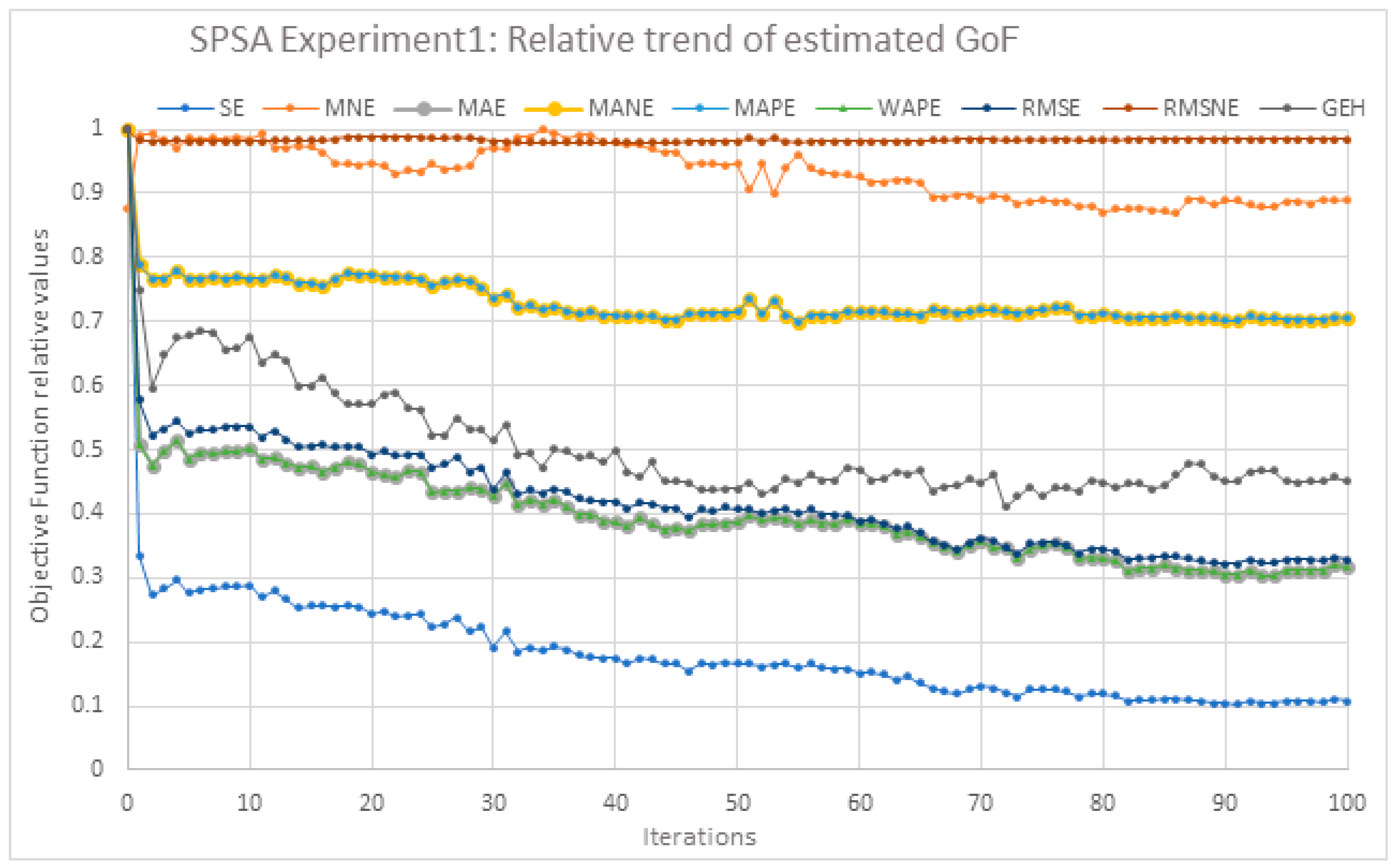
The goodness-of-fit adopted as the objective function is the SE squared error, i.e., the sum of the squared errors of the simulated and observed attractiveness, summed over all zones considered in the calibration and summed over all time frames.
o . f . = S E A s i m j ,   A o b s j = K × j D A s i m j A o b s j 2
Having defined the above measures of performance and goodness-of-fit, the mathematical formulation of the problem is as follows:
m i n β , λ   S E A s i m j ( β i , λ i ) ,   A o b s j = K × j D A s i m j ( β i , λ i ) A o b s j 2 Subject   to l β , i     β i     u β , i   i = 1 M l λ , i     λ i     u λ , i   i = 1 m
where
  • j = generic zone.
  • K = scaling factor to be calibrated based on the initial value assumed by the objective function.
  • βi = generic parameter in the distribution model to be calibrated.
  • λi = generic parameter in the nested model to be calibrated.
  • M = total number of βi parameters.
  • m = total number of λi parameters.
The calibration model has been formally integrated into the transport simulation by applying parameter multipliers. Within the Visum model, each Beta and Lambda parameter is associated with a corresponding multiplier. This setup allows the demand model to function using the product of the original parameters and their respective multipliers. The calibration process itself operates externally from the model, optimizing these multipliers and feeding the updated values back into the Visum model.

3.4. Selection of Optimization Algorithm

Calibrating travel demand models involves adjusting the model parameters to closely replicate observed travel patterns, a process that typically requires solving complex, nonlinear, and often stochastic optimization problems. Given the high dimensionality and potential non-convexity of the parameter space, the choice of optimization algorithms is critical to achieving reliable and efficient calibration results. In this context, three algorithms were selected for their complementary strengths: Simultaneous Perturbation Stochastic Approximation (SPSA), Particle Swarm Optimization (PSO), and Adaptive Moment Estimation (ADAM).
SPSA, introduced in [24], is particularly well suited for high-dimensional optimization problems where the objective function is noisy or expensive to evaluate. Its ability to approximate gradients with minimal function evaluations makes it an efficient choice for calibrating travel demand models, where simulation outputs can be computationally intensive. Moreover, SPSA’s stochastic nature helps it avoid local minima, enhancing the robustness of the calibration process.
The hyperparameters values adopted as the starting point are listed below:
  • a = 0.1 (initial step size).
  • c = 0.1 (perturbation size).
  • alpha = 0.602 (learning rate decay exponent).
  • gamma = 0.101 (perturbation decay exponent).
  • A = 10 (stability constant for learning rate).
  • Max No. iter = 100–200 (maximum number of iterations).
PSO, introduced in [25], inspired by the social behavior of biological swarms, offers a population-based, heuristic approach to exploring the parameter space. Its global search capability and simplicity in implementation make it effective in navigating complex, multimodal landscapes that are typical in travel demand calibration. PSO’s adaptability and parallel evaluation potential further support efficient convergence toward high-quality solutions.
The hyperparameters values adopted as the starting point are listed below:
  • No. particles = 20 (number of particles).
  • V = −0.1–0.1 (velocity).
  • w_max = 1 (initial inertia weight).
  • w_min = 0.005 (final inertia weight).
  • c1 = 0.5–2.5 (cognitive coefficient).
  • c2 = 0.5–2.5 (social coefficient).
  • Max No. iter = 50–100 (maximum number of iterations).
ADAM, introduced in [26], originally developed for training deep neural networks, combines the advantages of adaptive learning rates with momentum-based gradient descent. Its ability to dynamically adjust step sizes based on past gradients facilitates stable and rapid convergence, which is particularly useful in the context of gradient-based calibration tasks. ADAM’s efficiency and effectiveness in handling noisy gradients align well with the stochastic nature of travel demand model outputs.
The hyperparameters values adopted as the starting point are listed below:
  • α = 0.001 (learning rate).
  • β1 = 0.9 (first moment decay rate).
  • β2 = 0.999 (second moment decay rate).
  • epsilon = 10−8 (numerical stability term).
  • epsilon_grad = 10−2 (perturbation for numerical gradient estimation).
  • Max n. iter = 50–100 (maximum number of iterations).
All three algorithms discussed above—Simultaneous Perturbation Stochastic Approximation (SPSA), Particle Swarm Optimization (PSO), and Adaptive Moment Estimation (ADAM)—have been implemented with explicit consideration for variable constraints. To ensure that the solutions remain within the defined bounds, constraint handling is performed by clipping the candidate solutions at each iteration. This approach enforces the limits by adjusting any out-of-bound values back to the nearest permissible value, thereby maintaining feasibility throughout the optimization process.
Although various convergence criteria have been explored and implemented, the termination of the optimization algorithms was governed solely by the maximum number of iterations, irrespective of the values achieved by other convergence criteria. Convergence was monitored during the hyperparameter calibration experiments; however, some results from the regular experiments suggest that the convergence behavior warrants further investigation.
The three algorithms leverage their diverse methodological approaches, stochastic approximation, population-based search, and adaptive gradient optimization, to address the multifaceted challenges of travel demand model calibration. This selection aims to understand the different behaviors of the tested algorithms; indeed, each one presents a different balance between exploration and exploitation in the parameter space, different convergence speed, and different accuracy of solutions.
Before applying the three optimization algorithms, each underwent a dedicated calibration process to fine-tune their hyperparameters and ensure stable and efficient performance. The details of this calibration procedure, including parameter selection strategies and evaluation criteria, are provided in Appendix A.1.

4. Results

4.1. Experimental Design

Two sets of experiments were designed to evaluate the performance and effectiveness of the proposed model and algorithms.
The first set involved assigning random values to the parameters’ multipliers subject to the calibration problem. Specifically, random values between 0.250 and 2.00 were assigned to the three Beta multipliers, while values between 0.250 and 1.00 were assigned to the thirteen Lambda multipliers.
In the demand model, each parameter is multiplied by the corresponding parameter multiplier. Each set of parameter multipliers produces performance measures as the model output, which are then treated as observed data. These outputs are used to generate experiments in a controlled environment, where the true solution to the problem is known; specifically it corresponds to the set of perturbed parameters initially assigned.
The second set of experiments was created by introducing random perturbations directly to the observed measurement dataset, resulting in three additional calibration scenarios. In particular, the initial attractiveness values of the zones were randomly adjusted by ±10% in experiment 4, ±25% in experiment 5, and ±50% in experiment 6. These perturbed values were then normalized so that their total summed to 100%.
The following sections summarize the key findings derived from the experimental results. Comprehensive details regarding the experimental design are provided in Appendix A.3. The detailed results for each individual experiment are available in Section 4.2. Section 4.3 presents the main conclusions and insights obtained from the analysis of the experimental outcomes.

4.2. Analysis of the Results of Individual Experiments

4.2.1. Experiment 1 Results

1.
Analysis of Algorithm performances
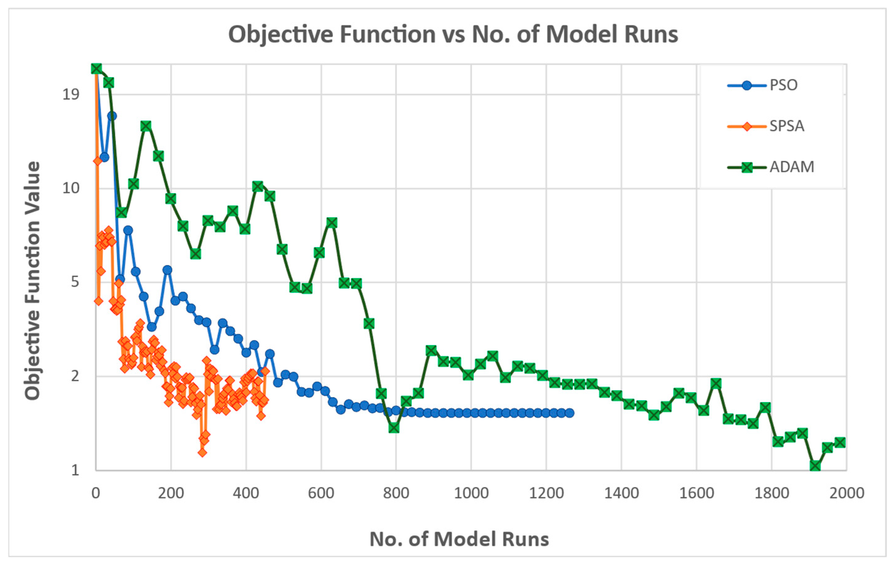
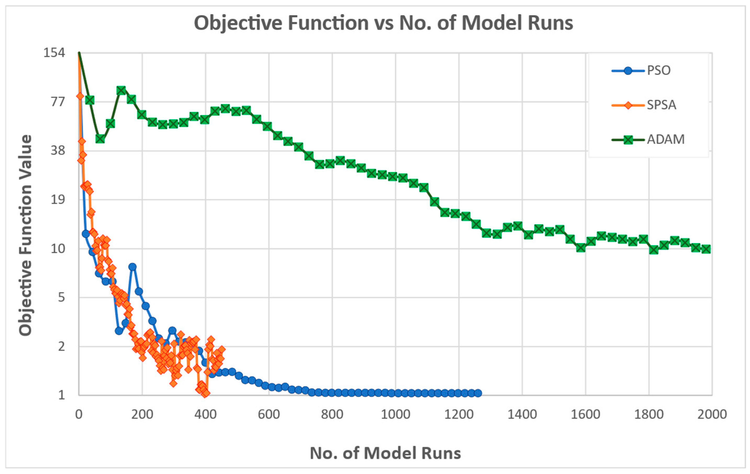
Figure 2 reported below shows a comparison of the three algorithms’ performances in terms of the trend of the objective function value over model runs. The graph shows the objective function value on the y-axis, plotted against the number of model runs (x-axis), for three algorithms: PSO (blue), SPSA (orange), and ADAM (gray). For each iteration, SPSA uses 3 model runs, PSO uses 21 model runs, and ADAM uses 33 model runs.
  • ADAM starts with a high objective value (~19), much higher than the others, indicating poorer initial solutions.
  • It demonstrates non-monotonic but consistent long-term improvement—large fluctuations are observed especially in the first half, likely due to high learning rates or adaptive updates.
  • After circa 700 model runs, it drops below the PSO and SPSA lines and continues improving.
  • It ultimately reaches the lowest final value (~1.2), the best performance overall.
  • This behavior is typical of adaptive gradient-based optimizers, which may initially overshoot but gain precision over time.
  • PSO shows a smooth and steady decrease until around 800–900 runs, after which it plateaus (no further improvements).
  • The final value stabilizes around 1.8, which is better than SPSA but worse than ADAM.
  • This behavior suggests early convergence to a local minimum or premature exploitation, a known issue in PSO without diversity management.
  • SPSA begins with relatively good performance and quickly improves within the first 100–200 runs.
  • It then enters a highly noisy region with erratic fluctuations and small-scale improvements.
  • It appears to hover around 2.0, with some outliers but no strong long-term descent.
  • This suggests that SPSA converges fast but lacks precision in the later stages without tighter tuning of the perturbation schedule.
The key observations are summarized in Table 1 below.
2.
Objective Function and other KPIs
Table 2 reported below shows the minimum objective function and estimated KPI values for each tested algorithm, in comparison with the same values with the initial condition.
The results of calibration experiment 1 show that the ADAM algorithm consistently outperformed SPSA and PSO across nearly all key performance indicators. Specifically, ADAM achieved the lowest values for the objective function and standard error metrics (e.g., MAE, RMSE, MAPE, WAPE), indicating a higher overall calibration accuracy. Moreover, ADAM found a solution significantly closer to the known true parameter set, both in terms of Euclidean distance (0.733) and correlation (0.816), suggesting a superior capability in reproducing the underlying model structure. SPSA, while less accurate on most metrics, delivered the best result for the GEH statistic (0.010), which in this particular case is not as relevant as it is when applied to traffic flow. PSO exhibited intermediate performance without clearly dominating in any metric. These findings support the selection of ADAM as the most effective algorithm for accurate and reliable calibration in this context, while SPSA may still be preferable in applications where matching observed flows is a priority.
Finally, it can be noted that except for MNE, RMSNE, and GEH, the minimum of all the other computed KPIs correspond to the minimum of the objective function.
Among the tested algorithms, ADAM consistently outperformed SPSA and PSO across almost all KPIs, including objective function value, absolute and percentage-based error metrics, and the closeness to the true solution. SPSA showed a strong performance in minimizing the GEH statistic, indicating its capability in preserving volume distributions, while PSO exhibited mid-level performance without excelling in any particular metric.
3.
Parameter recovery performance
Table 3 reported below provides a clear picture of the parameter recovery performance of SPSA, PSO, and ADAM against the true parameter values.
The analysis of the Euclidean distance to the true solution confirms ADAM’s superior accuracy in matching the true parameter vector. Additionally, ADAM shows the highest correlation to the true vector (0.816), indicating that it better captures the overall shape and pattern of the parameter set. In more detail, ADAM is the closest for 9 out of 16 parameters, SPSA is the closest for 5 out of 16 (including one exact match), and PSO is the closest for 2 out of 16 (but never much better than the others).
The recovered parameter vectors were compared against the known true values to assess each algorithm’s capability in reconstructing the model structure. ADAM achieved the lowest Euclidean distance (0.733) and the highest correlation (0.816) with the true solution, indicating its superior ability to recover the correct parameter patterns. It was closest to the true value for 9 out of 16 parameters, particularly excelling in core behavioral coefficients such as travel time, walking, and student-related LAMBDA terms. SPSA showed moderate recovery quality and exactly matched one parameter (LAMBDA_RPLUSMP), while PSO performed less accurately overall. Some parameters, such as BETA_TRANSFER and LAMBDA_APP, were underestimated by all algorithms, suggesting lower sensitivity or identifiability in the calibration setup. These findings reinforce ADAM’s suitability for reliable and interpretable model calibration.

4.2.2. Experiment 2 Results

1.
Analysis of Algorithm performances
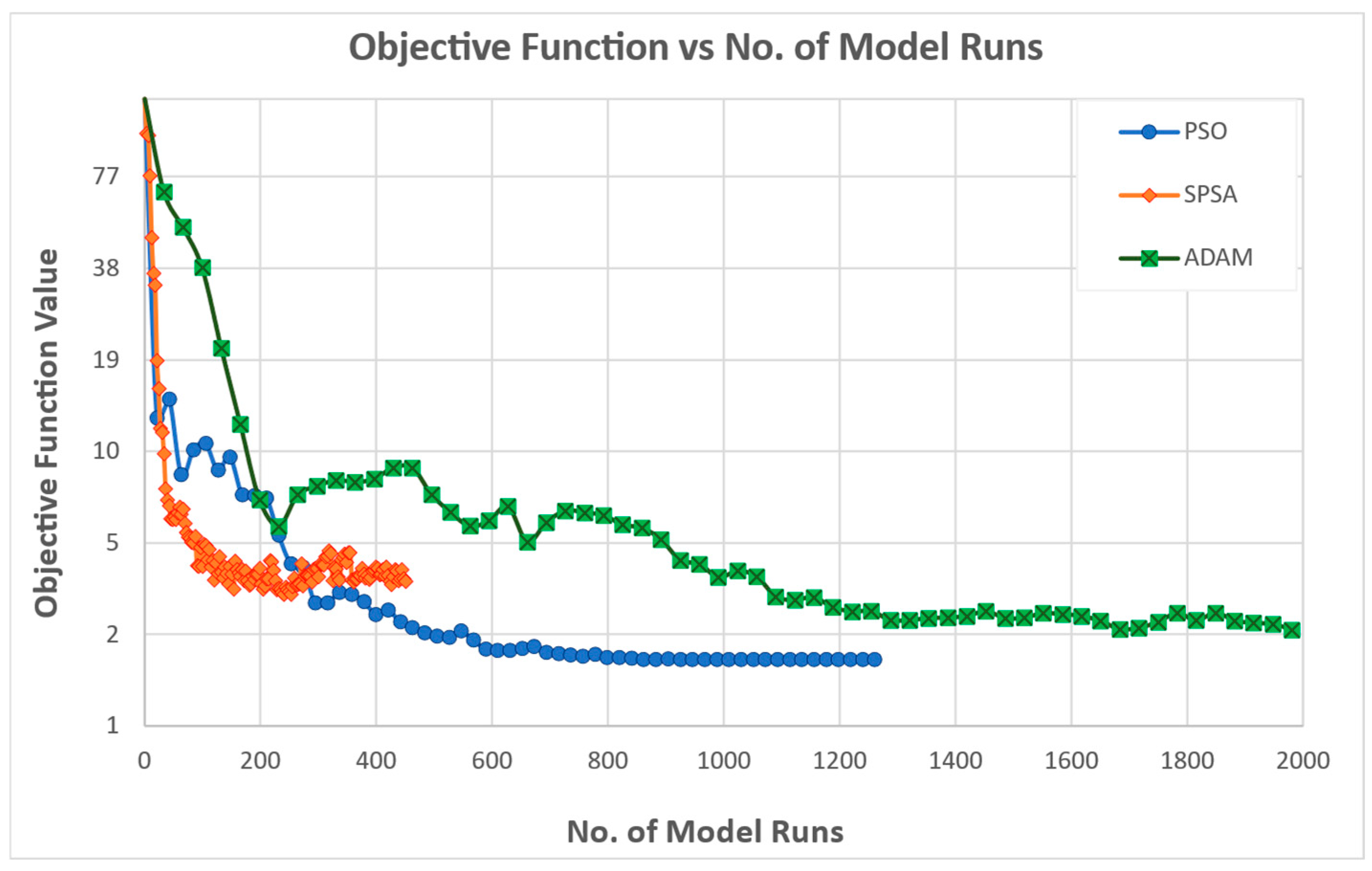
Figure 3 reported below shows a comparison of the three algorithms’ performances in terms of the trend of the objective function value over model runs for experiment 2.
  • PSO shows smooth and consistent convergence to a low objective function value.
  • Exhibits fast early improvements, reaching a stable value quickly.
  • Maintains low noise in its trajectory, indicating stable performance.
  • Long-term improvement is limited after initial convergence.
  • SPSA demonstrates fast early improvements but with significant noise.
  • Lacks smooth convergence, with fluctuations in the objective function value.
  • High noise in the trajectory suggests instability.
  • Long-term improvement is minimal after initial improvements.
  • ADAM achieves the best final objective value over a longer period.
  • Convergence is not smooth, with moderate noise present.
  • Shows significant long-term improvement, gradually decreasing the objective function value.
  • The trajectory indicates consistent optimization over time.
The key observations are summarized in Table 4 below.
2.
Objective Function and other KPIs
Table 5 reported below shows the minimum objective function and estimated KPI values for each tested algorithm, in comparison with the same values with the initial condition.
The results of calibration experiment 2 show that PSO achieves the lowest objective function value (1.990), indicating the best optimization performance among the three algorithms. ADAM has a moderate objective function value (2.485), performing better than SPSA but not as well as PSO. SPSA exhibits the highest objective function value (3.375), suggesting that it is less effective in optimization compared with the other algorithms. PSO also produces the best values for almost all the KPI metrics.
Unexpectedly, the solution found by PSO is not the closest to the known true parameter set in terms of Euclidean distance (1.508) and correlation (0.816), suggesting superior capability in reproducing the underlying model structure. SPSA has the lowest distance (1.201), which may indicate a closer fit to the true solution despite higher objective function value. PSO has the highest distance (1.508), whereas ADAM is moderate (1.334). SPSA has the highest correlation (0.704), suggesting better overall correlation performance. PSO and ADAM have lower correlation values.
PSO demonstrates superior optimization performance with the lowest objective function value and exceptional accuracy across multiple KPIs, including SE, MNE, MAE, MANE, MAPE, WAPE, and RMSE. Despite having a higher GEH statistic and distance, it maintains a strong correlation, making it the most reliable algorithm. ADAM follows with a moderate performance, while SPSA, despite having a lower distance, struggles with higher objective function value and less accuracy. Overall, PSO appears to be the best choice for this optimization task due to its precision and reliability.
3.
Parameter recovery performance
Table 6, reported below, provides a clear picture of the parameter recovery performance of SPSA, PSO, and ADAM against the true parameter values.
The analysis of the Euclidean distance to the true solution shows SPSA’s superior accuracy in matching the true parameter vector.
SPSA performed well for parameters like BETA_WALK, BETA_TRANSFER, and LAMBDA_EMP where it was closest to the true value. It had the highest count of best solutions (6 out of 16), indicating a strong performance in multiple areas.
PSO showed a strong performance for parameters like BETA_TT, LAMBDA_EOP, and LAMBDA_PRIMPUPIL. It also had the highest count of the best solutions (6 out of 16), demonstrating its robustness across different parameters.
ADAM was the best for parameters like LAMBDA_NEOP, LAMBDA_RPLUSOP, and LAMBDA_ROP. While it had fewer best solutions (4 out of 16), it still showed a competitive performance in certain areas.
Overall, SPSA and PSO were the most consistent algorithms, each securing the best solution for six parameters. ADAM, though slightly behind, still offered competitive solutions for specific parameters.

4.2.3. Experiment 3 Results

1.
Analysis of Algorithm performances
Figure 4 reported below shows a comparison of the three algorithms’ performances in terms of the trend of the objective function value over model runs for experiment 3.
  • PSO exhibits a smooth and rapid decline in the objective function value, particularly in the early stages (first 200 model runs).
  • Achieves a stable and low objective function value quickly and maintains it throughout the remaining model runs.
  • Demonstrates smooth convergence with minimal fluctuations.
  • SPSA shows a fast initial decrease in the objective function value, similar to PSO. However, it has more fluctuations and noise in its trajectory compared with PSO, even though it finds the best solution.
  • After the initial rapid improvement, the objective function value stabilizes but with noticeable variability.
  • ADAM starts with a high objective function value and decreases gradually over the model runs.
  • Demonstrates moderate noise with a less smooth trajectory compared with PSO.
  • Shows long-term improvement, continually decreasing the objective function value over time, but at a slower rate than PSO and SPSA.
Overall, SPSA achieves the best solution while PSO presents the most stable final objective function value, with smooth convergence. SPSA shows fast early improvements but with higher noise, while ADAM provides long-term improvement with moderate noise. The key observations are summarized in Table 7 below.
2.
Objective Function and other KPIs
Table 8 reported below shows the minimum objective function and estimated KPI values for each tested algorithm, in comparison with the same values with the initial condition.
The results of calibration experiment 3 show that based on the analysis of the KPIs, SPSA consistently achieves good values across all the metrics, and the best value of the objective function, SE, MAPE, WAPE, and GEH.
PSO achieves the best performance across almost all the metrics, excluding the lowest objective function value (1.237), MNE, MAE, MANE, RMSE, and Euclidean distance (0.649). It can be noted that the solution found by the PSO presents the minimum distance from the true solution, highlighting again that the squared error may not be the best goodness-of-fit measure.
ADAM presents a consistent and gradual decreasing trend. However, due to a bad performance in the early stage and a slow rate in the objective function’s reduction, in this experiment it is outperformed by SPSA and PSO.
3.
Parameter recovery performance
Table 9 reported below provides a clear picture of the parameter recovery performance of SPSA, PSO, and ADAM against the true parameter values.
The analysis of the Euclidean distance to the true solution shows PSO’s superior accuracy in matching the true parameter vector.
PSO performed well for parameters like BETA_TT, BETA_WALK, BETA_TRANSFER, and LAMBDA_EOP where it was closest to the true value. It had the highest count of best solutions (7 out of 16), indicating strong performance in multiple areas.
SPSA showed also good performance. It also had the highest count of the best solutions (6 out of 16), demonstrating its robustness across different parameters.
ADAM in this experiment did not perform well and it had only the best solution for one parameter (1 out of 16).
Overall, PSO has the highest count of parameters closest to the true values, indicating it provides the best overall approximation to the true solution. SPSA also performs well, particularly for several parameters. ADAM is less effective in approximating the true solution compared with the other two algorithms.

4.2.4. Experiment 4 Results

1.
Analysis of Algorithm performances
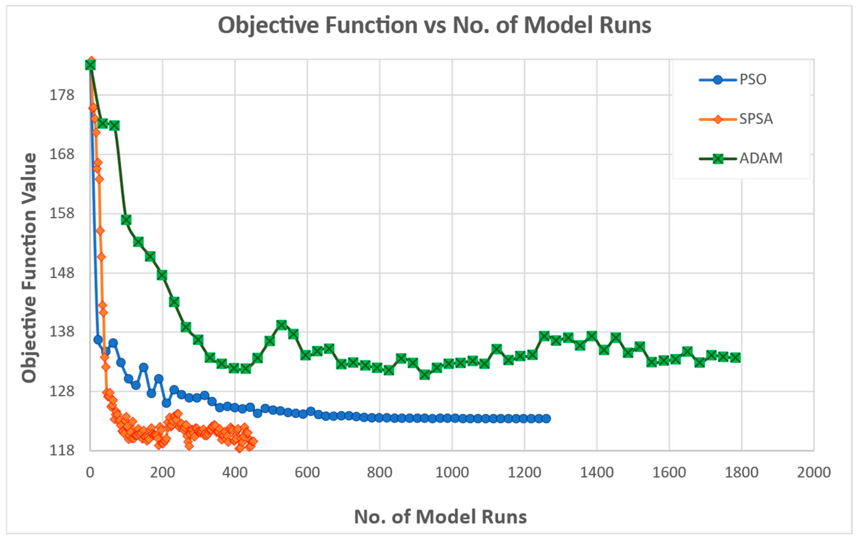
Figure 5 reported below shows a comparison of the three algorithms’ performances in terms of the trend of the objective function value over model runs for experiment 4.
  • PSO Demonstrates smooth convergence with minimal fluctuations.
  • Shows a consistent performance with a stable trajectory after initial rapid improvements.
  • SPSA Shows fast early improvements in the objective function value.
  • Exhibits more fluctuations and noise in its trajectory compared with PSO.
  • Achieves a stable objective function value after initial rapid improvements, but with noticeable variability. Achieves the lowest final objective function value.
  • ADAM Starts with a high objective function value and decreases gradually over the model runs.
  • Demonstrates moderate noise with a less smooth trajectory compared with PSO.
  • Shows long-term improvement, continually decreasing the objective function value over time, but at a slower rate than PSO and SPSA.
Overall, SPSA achieves the best final objective function value and although it is noisy it is always lower than the PSO curve. SPSA shows fast early improvements but with higher noise, while ADAM provides long-term improvement with moderate noise. PSO presents, as expected, a smooth convergence to higher values.
The key observations are summarized in Table 10 below.
2.
Objective Function and other KPIs
Table 11 reported below shows the minimum objective function and estimated KPI values for each tested algorithm, in comparison with the same values with the initial condition.
The results of calibration experiment 4 show that based on the analysis of the KPIs, SPSA consistently achieves the best performance across many of the metrics, including the lowest objective function value (118.381), SE, MAE, WAPE, RMSE, and GEH. ADAM achieves the best results for MNE, MANE, MAPE, RMSNE, and correlation coefficient. PSO is identified as the best algorithm among the three.
Based on the analysis of the KPIs, SPSA consistently achieves the best performance across most metrics, including the lowest objective function value. Therefore, SPSA is identified as the best algorithm among the three.

4.2.5. Experiment 5 Results

1.
Analysis of Algorithm performances
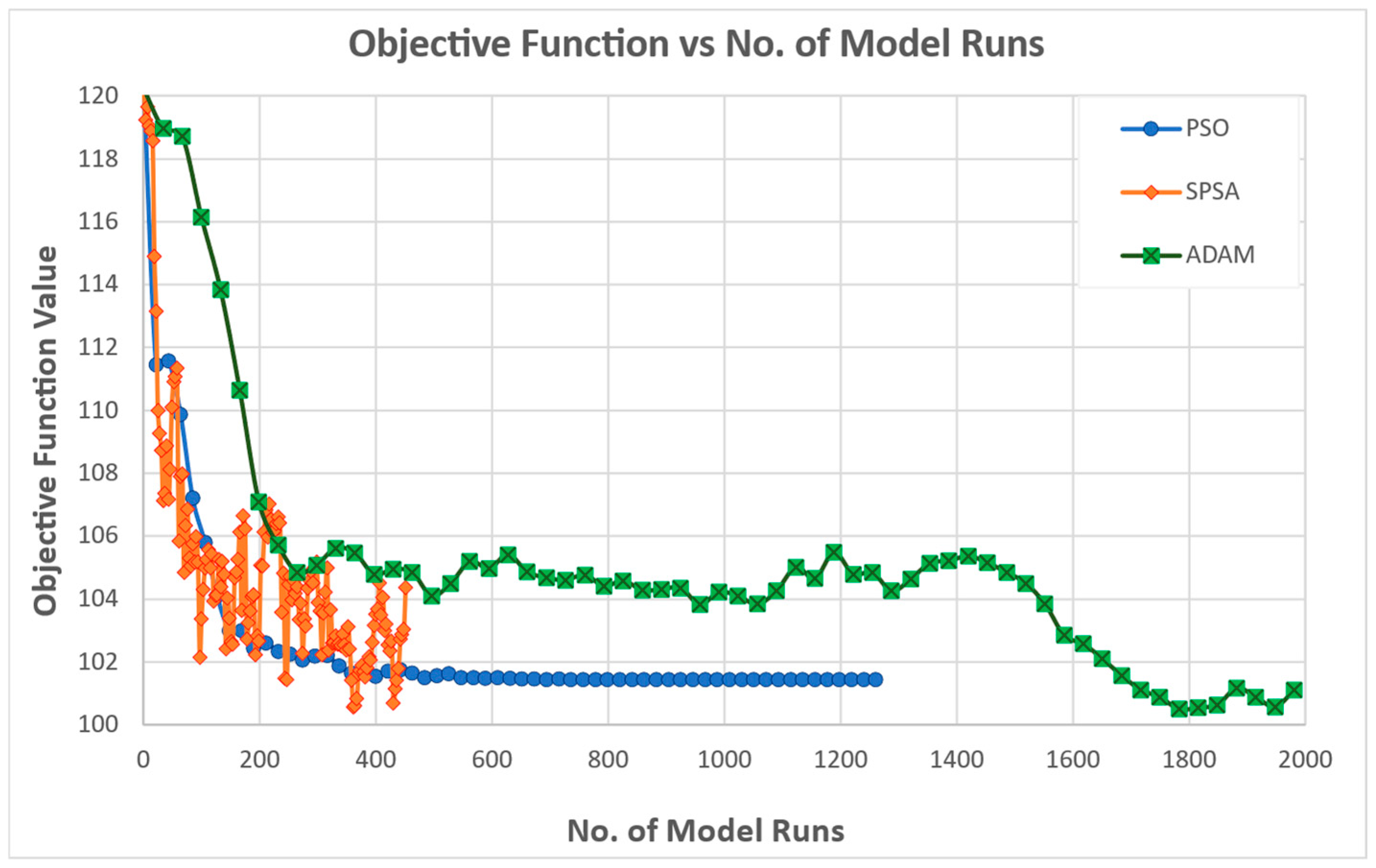
Figure 6 reported below shows a comparison of the three algorithms’ performances in terms of the trend of the objective function value over model runs for experiment 5.
  • PSO quickly achieves stability with a final objective function value of 101.403.
  • Demonstrates smooth convergence with minimal fluctuations.
  • Shows a consistent performance with stable trajectory after initial rapid improvements.
  • SPSA Shows fast early improvements in the objective function value.
  • Exhibits more fluctuations and noise in its trajectory compared with PSO.
  • Achieves a stable objective function value after initial rapid improvements, but with noticeable variability. The best value found is equal to 100.562
  • ADAM Starts with a high objective function value and decreases gradually over the model runs.
  • Demonstrates moderate noise with a less smooth trajectory compared with PSO.
  • Shows long-term improvement, continually decreasing the objective function value over time, but at a slower rate than PSO and SPSA.
  • It finds the best solution for this experiment, with an objective function value of 100.493
Overall, ADAM achieves the best final objective function value, even if with a lengthy process. SPSA also achieves a good solution, though it has a noisy process and it is often lower than the PSO curve. SPSA shows fast early improvements but with higher noise, while ADAM provides long-term improvement with moderate noise. PSO presents, as expected, a smooth convergence to higher values.
The key observations are summarized in Table 12 below.
2.
Objective Function and other KPIs
Table 13 reported below shows the minimum objective function and estimated KPI values for each tested algorithm, in comparison with the same values with the initial condition.
The results of calibration experiment 5 show that based on the KPIs, ADAM appears to be the best algorithm overall, achieving the lowest objective function value and excelling in several other metrics such as MAPE, RMSE, and correlation coefficient. Despite its higher standard error, SPSA’s performance in key areas and its strong correlation coefficient make it the most effective choice among the three algorithms.
Objective function:
  • ADAM achieves the lowest objective function value (100.493), indicating effective optimization performance.
  • SPSA follows with a slightly higher value (100.562).
  • PSO has the highest objective function value (101.430) among the three.

4.2.6. Experiment 6 Results

1.
Analysis of Algorithm performances
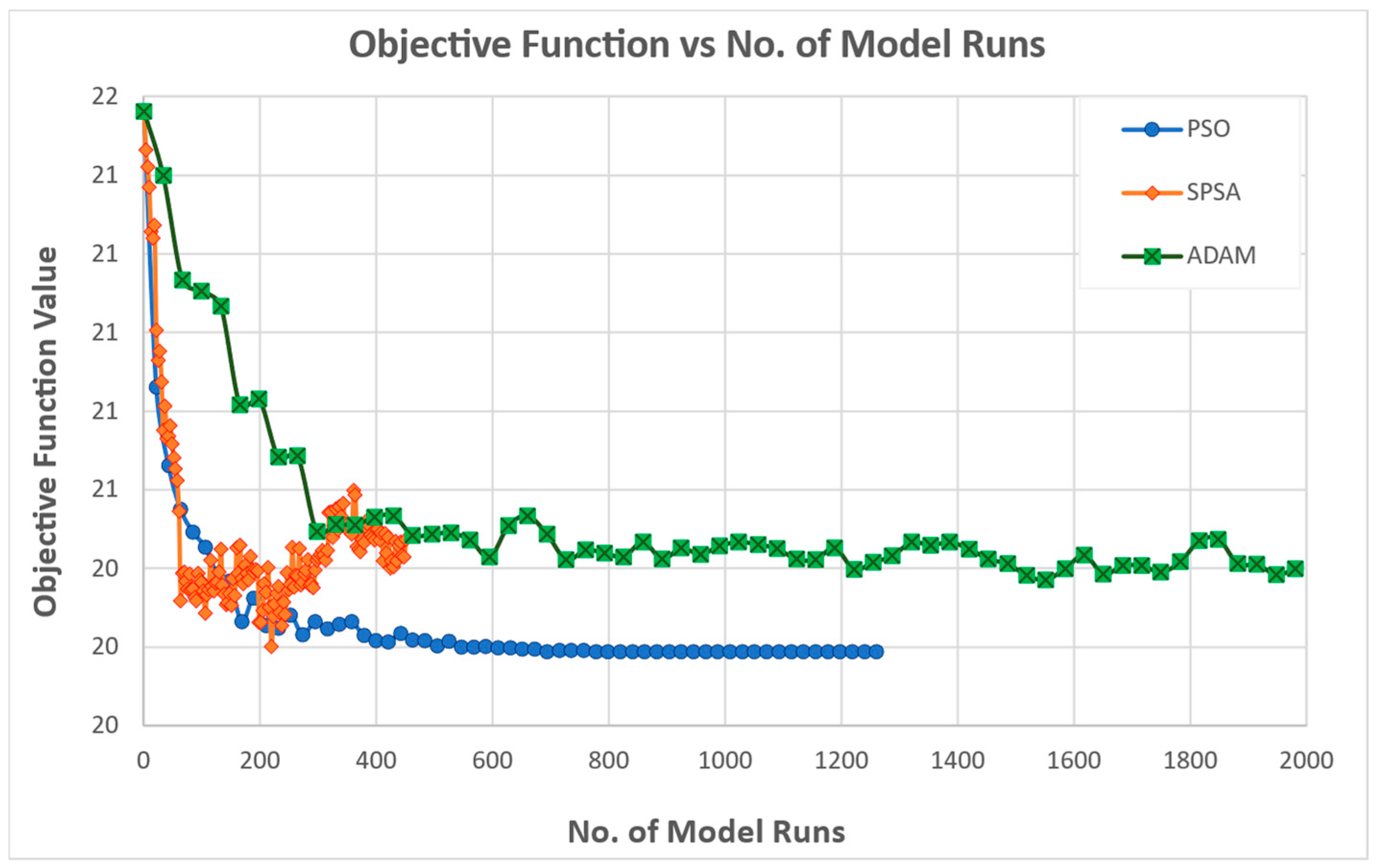
Figure 7 reported below shows a comparison of the three algorithms’ performances in terms of the trend of the objective function value over model runs for experiment 6.
  • PSO achieves the lowest final objective function value around 20.188.
  • Exhibits smooth convergence with minimal fluctuations after initial rapid improvements.
  • Stabilizes early in the process and maintains a consistent trajectory throughout the model runs.
  • SPSA demonstrates fast early improvements, quickly reducing the objective function value.
  • Shows significant fluctuations and noise in its trajectory, indicating variability in convergence.
  • Stabilizes at a slightly higher objective function value than PSO after initial fluctuations.
  • ADAM starts with a high objective function value and decreases gradually over the model runs.
  • Exhibits a less smooth trajectory with moderate noise compared with PSO.
  • Shows long-term improvement, continually decreasing the objective function value over time, but at a slower rate and stabilizes at a higher value than both PSO and SPSA.
Overall, PSO demonstrates the best performance with the lowest final objective function value and smooth convergence, making it the most reliable algorithm in terms of stability and early stabilization. SPSA shows fast early improvements but with significant noise, indicating variability in its trajectory. ADAM, while showing long-term improvement, stabilizes at a higher objective function value and exhibits moderate noise, suggesting it is less effective compared with PSO and SPSA. Thus, in this experiment PSO stands out as the most effective algorithm for achieving the optimal performance.
The key observations are summarized in Table 14 below.
2.
Objective Function and other KPIs
Table 15 reported below shows the minimum objective function and estimated KPI values for each tested algorithm.
The results of calibration experiment 6 show that based on the analysis of the KPIs, PSO consistently achieves the best performance across most metrics, including the lowest objective function value (20.188), SE, MNE, MAE, MANE, MAPE, WAPE, RMSE, and RMSNE. Despite having a higher GEH, the overall performance of PSO in terms of accuracy and error metrics makes it the best algorithm among the three.

4.3. General Analysis of Results

4.3.1. Convergence Dynamics

ADAM consistently starts with a high objective value due to its aggressive adaptive updates, leading to large initial fluctuations. However, its precision increases over time, producing substantial long-term improvements and the lowest final values in experiments 1 and 5.
PSO exhibits smooth, rapid early declines in the objective function, stabilizing quickly and maintaining minimal noise thereafter. This reliable exploitation is evident in experiments 2, 3, 6, and to some extent 4, where PSO attained the lowest or near-lowest final values.
SPSA shares PSO’s rapid initial gains but suffers from higher noise and variability throughout, as seen in all experiments. It often plateaus early (experiments 1–2) or oscillates around its best solution (experiments 3–4), highlighting challenges in fine-tuning its perturbation schedule for sustained descent.
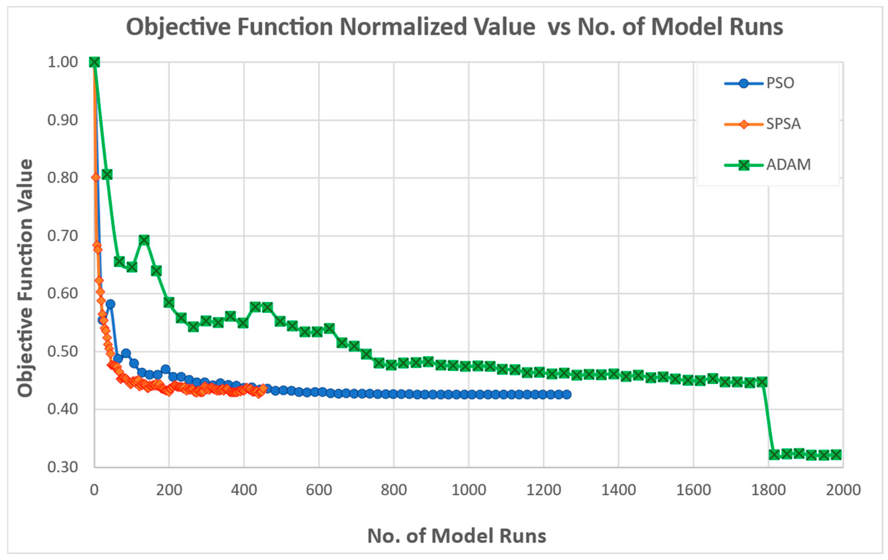
Figure 8, reported below, illustrates a comparison of the three algorithms’ performances in terms of the trend of the objective function normalized value, averaged over all six experiments, over model runs. The graph shows the objective function value on the y-axis, plotted against the number of model runs (x-axis), for three algorithms: PSO (blue), SPSA (orange), and ADAM (gray). It can be noted that for each iteration, SPSA uses 3 model runs, PSO uses 21 model runs, and ADAM uses 33 model runs.
Table 16 reported below summarizes the key observations obtained by generalizing the observed behaviors over all six experiments.

4.3.2. Optimization Performance, Objective, and KPIs

ADAM shines when the calibration objective aligns with the squared error metrics: it attained the best objective values in experiment 1 (≈1.2) and experiment 5 (100.493) and dominated most MAE, RMSE, and percentage error KPIs in those runs.
PSO outperformed both alternatives in objective value and most error metrics in experiments 2 (1.99) and 6 (20.188), demonstrating its robustness across a variety of calibration landscapes.
SPSA led only intermittently—most notably minimizing the GEH statistic (experiment 1) and claiming the lowest objective in experiments 3 (1.217) and 4 (118.38)—but its noisy convergence often prevented it from sustaining those gains.

4.3.3. Parameter Recovery Accuracy

ADAM achieved the closest match to the true parameter vector in exp. 1 (Euclidean distance 0.733, correlation 0.816) and was the best for 9 out of 16 parameters, illustrating its ability to reconstruct the underlying model structure when allowed sufficient iterations.
PSO excelled in exp. 3 (distance 0.649) and exp. 6, and led in 7 out of 16 parameters in exp. 3, indicating that its stable search can accurately localize parameters when the landscape is amenable to swarm exploration.
SPSA demonstrated the strongest recovery in exp. 2 (distance 1.201) and outperformed in several individual parameters across experiments—particularly those related to transfer and walking utilities—but lacked consistency in overall distance metrics.

5. Discussion

5.1. Algorithm Setups, Hardware, and Performances

The algorithm configurations used in this study are based on those determined during the hyperparameter calibration phase, with the exception of the maximum number of iterations, which was increased for the experimental runs.
The stopping criteria were set as follows: parameter variation lower than 1 × 10⁻³ or objective function variation lower than 1 × 10⁻⁵ with respect to the previous iteration. These criteria were met during the hyperparameters’ calibration, leading to the setting of the maximum number of iterations.
During the experiments’ execution, the maximum number of iterations was raised from 100 to 150 for SPSA, and from 50 to 60 for both PSO and ADAM. This adjustment was necessary due to the initial objective function values being higher than those observed during calibration. Nevertheless, despite the increased iteration limits, the solutions produced by all three algorithms remain significantly distant from the true optimal solutions.
This suggests that future experiments should consider further increasing the maximum number of iterations.
All experiments were conducted on a machine equipped with an Intel® Core™ Ultra 9 Processor 285 K (36 M Cache, up to 5.70 GHz) and 64 GB of RAM. On this hardware, a single model evaluation requires approximately one minute. Taking into account both the calibration and experimental phases, the total computational time amounts to roughly 1000 h.
It is also worth noting that, at the current stage of the research, the use of a kriging surrogate meta-model for approximating the objective function has not been pursued. While surrogate modeling—particularly kriging—can significantly reduce computational costs by approximating the objective function based on a limited number of model evaluations, it introduces an additional layer of modeling complexity and potential approximation error. In this study, the focus has been placed on assessing the optimization algorithms in their direct application to the true, high-fidelity model, without the influence of surrogate-induced biases. This choice allows for a more transparent evaluation of the algorithms’ behavior and performance characteristics in solving the original problem. Nonetheless, incorporating surrogate models such as kriging remains a promising avenue for future work, especially in contexts where computational demands become prohibitive.
Across the six calibration experiments, distinct patterns emerge in the behavior and performance of the three optimizers, reflecting inherent trade-offs between convergence speed, stability, and final accuracy.

5.2. Practical Implications

Trade-off between speed and precision: PSO’s swift, low-noise descent makes it ideal for time-constrained calibrations requiring a good—but not necessarily the best—fit.
Noisy but flexible: SPSA can be leveraged when alternative goodness-of-fit measures are prioritized, though it demands careful tuning to mitigate variability.
Long-run accuracy: ADAM is preferable when the computational budget allows for many iterations and when minimizing squared errors and recovering true parameters are critical. Introducing and testing ADAM as an alternative optimizer for calibration is a primary methodological contribution.

5.3. Findings

The calibration experiments reveal that no single optimizer uniformly dominates across all criteria; instead, each offers strengths tailored to specific calibration priorities:
PSO provides the most reliable and rapid convergence to low objective values with minimal noise, making it well suited for scenarios requiring consistent, fast calibration.
SPSA delivers competitive early improvements and excels in some metrics, but demands tighter perturbation control to achieve stability and precision.
ADAM is the method of choice for achieving the lowest squared error objectives and the superior recovery of true parameter vectors when ample iterations are available.
Ultimately, the selection of an optimization algorithm should align with the calibration goals—whether that is maximizing overall accuracy, ensuring stability under tight iteration budgets, or targeting specific distributional fit measures.
Under the conditions of limited computational resources or strict time constraints, SPSA is preferable, as it delivers faster initial performance gains.
It should also be noted that certain model parameters cannot be reliably identified given the selected calibration targets. For instance, in experiment 1.1, all three algorithms consistently underestimated the BETA_TRANSFER parameter, likely because the zonal attractiveness indicator contains insufficient information to capture transfer penalties. Similarly, parameters such as the LAMBDA values for demand segments related to education activities are difficult to identify, owing to the limited contribution of these segments to the overall demand and, consequently, to the zones’ attractiveness.
Some limitations stem from the model’s original formulation. At the outset of the study, we chose to use the ABM supplied by PTV as an example, rather than investing time in developing a more specific and detailed model.
This decision was guided by two main considerations. First, using the PTV model facilitates reproducibility, as it is a widely accessible platform. Second, it supports a broader research objective: developing a calibration procedure that can be applied to models transferred from other contexts. In such situations, modifying the transferred model is often impractical; our aim is therefore to enable calibration even when the underlying model is simplistic or sub-optimally specified.

5.4. Future Research Directions

Further research is recommended across several key areas, with the aim of enhancing both the travel demand modeling aspects and the calibration and optimization frameworks employed in this study.
  • Enhancements to the travel demand model:
    • Incorporation of a higher temporal resolution: Future work should explore the integration of performance measures at a finer temporal granularity—such as by specific time slots or periods within the day. This would allow for a more accurate representation of travel behavior and model sensitivity to temporal variations in demand.
    • Extension to additional demand sub-models: The calibration framework could be extended to encompass other components of the demand model, starting with the mode choice sub-model. This is particularly relevant in the context of the agent-based model (ABM) used in this research, where destination and mode choices are modeled together in a nested structure. A more comprehensive calibration approach could lead to improved consistency and predictive power across interrelated sub-models.
  • Advancements in the calibration framework:
    • Utilization of emerging mobility data sources: Future studies should investigate the integration of alternative data sources—including crowd-sourced mobility data and opportunistically collected individual movement traces—as inputs for generating more robust and diverse performance measures. These data could help capture a wider range of travel behaviors and increase the realism of calibration scenarios.
    • Development of novel goodness-of-fit metrics: There is also scope for defining new formulations of goodness-of-fit indicators or the definition of multi-objective functions that better reflect the complexity of model behavior and user interactions in ABMs. These metrics should aim to balance statistical rigor with computational efficiency, while being sensitive to spatial and temporal heterogeneity in observed patterns.
  • Improvements in the optimization process:
    • Assessment of convergence behavior: Further exploration is needed to understand the ability of optimization algorithms to identify global optima as the maximum number of iterations is increased. Based on these insights, appropriate convergence criteria can be defined to ensure reliable termination conditions.
    • Algorithmic enhancements: Lastly, future research should consider possible enhancements or adaptations of the employed optimization algorithms to improve performance, scalability, and robustness. This may involve hybrid approaches, adaptive parameter tuning, or incorporating problem-specific heuristics to accelerate convergence and improve solution quality.
  • Testing the framework on a real-world larger network:
    • Challenges: Increasing the size and complexity of the agent-based model (ABM) would substantially raise the computational burden for each simulation run. This, in turn, would extend the total execution time required for the calibration process, as a larger number of parameter combinations must be evaluated. In practical terms, this means that scaling up to more detailed or larger-scale ABMs could result in calibration procedures that take days or even weeks to complete, depending on the available computational resources. Moreover, the real-world applications may present data quality issues (e.g., missing or noisy connections, the over- or under-representation of some specific users’ segments).
    • The possible solutions to be investigated to overcome the computational challenges are the algorithmic enhancements mentioned above, including approximation techniques, employing heuristic approaches to approximate key metrics without requiring full-scale computation on the entire network, distributed computing, adapting the framework for a high-performance computing environment, and domain-specific constraints, incorporating prior knowledge about parameter values to limit the search space and computational load.
    • Possible solutions to be investigated to overcome the data quality include the following: robust data preprocessing pipelines, integrating multiple data sources to improve completeness and accuracy, and applying noise reduction or filtering techniques to mitigate measurement errors.

6. Conclusions

This paper has presented a general methodology for the aggregate calibration of transport models applied to the case of destination choice models, embedded in an activity-based model. Using a test network, this paper utilizes processed data collected from cell phone calls and/or data collected from apps installed on smartphones. Although the characterization of trips with regard to the trip purpose and mode of transport is still controversial, the processing of this data provides OD trip matrices marked by a good level of temporal and spatial characterization.
The calibration task is approached as a simulation optimization process, which aims to minimize the deviations between the model simulation output and the observed data, which have been hypothesized.
Three different types of algorithms have been used, evaluated, and compared: Simultaneous Perturbation Stochastic Approximation (SPSA), Particle Swarm Optimization (PSO), and Adaptive Moment Estimation (ADAM).
Based on the literature reviewed, the use of the ADAM optimizer in this specific calibration context appears to be novel, as no prior studies were identified that have explored its application for this purpose. Introducing and systematically testing ADAM as an alternative to more conventional optimization algorithms represents a primary methodological contribution of this study, which is centered on calibration methodology rather than on the development of a new demand model. Introducing ADAM not only broadens the set of available tools for model calibration but also provides an initial benchmark for evaluating the potential advantages and limitations of adaptive gradient methods in this domain.
Also, tests were performed to calibrate the three optimization algorithms’ hyperparameters; the squared error and several goodness-of fit values have been calculated.
The following deductions were made on the latter. The MNE can also present a negative correlation with the distance (between the solutions and the true solution), indicating that MNE is not suitable to be used as a GoF. The RMSNE and SE present the worst performances. Different GoF tests perform differently with different algorithms, such as GEH and the correlation coefficient. MAE, MANE, MAPE, and WAPE rank in the middle to highly. The RMSE always shows a strong correlation with the distance between the computed solutions and the true solution.
The calibration experiments reveal that no single optimizer uniformly dominates across all criteria; instead, each offers strengths tailored to specific calibration priorities. It is interesting to note that ADAM is preferable when the computational budget allows for many iterations (and model runs) since it presents the ability to ensure long-term objective function improvements.
On the practical side, the approach presented here allows an efficient calibration of destination choice model parameters by using cheap and readily available data. Given the limited data with which travel models are often estimated in practice, the proposed framework appears to be valuable.
The method can easily be extended to use other sources of available opportunistic data to calibrate other sub-models’ parameters.
The proposed methodology for aggregate model calibration has wide-ranging applications, suitable for various types of models regardless of their specific structure or scale. Crowd-sourced individual mobility data has become a valuable resource for updating or calibrating transport system models. These technological developments further expand the potential for applying aggregate calibration using crowd-sourced mobility data.
A key limitation of the proposed calibration approach lies in the inherent characteristics of simulation optimization. This typically requires numerous evaluations of the objective function, each requiring a full execution of the transport model. When applied to real-world networks with a large size, this process can become computationally intensive and time-consuming. As the size and complexity of the network increase, so does the computational burden, potentially limiting the practicality of the method for large-scale applications without significant strategies to increase the algorithms’ performances.
However, the approach developed here is not only more rigorous but also more efficient than the manual trial and error procedures. Also, the result is the first to develop a wider framework for the aggregate calibration of a full transport simulation model that is less costly and more accurate, using crowd-sourced individual and/or opportunistic mobility data.

Author Contributions

Conceptualization, V.B.; methodology, V.B. and A.G.; software, V.B. and A.G.; validation, V.B. and A.G.; formal analysis, V.B. and A.G.; investigation, V.B. and A.G.; resources, V.B. and A.G.; data curation, V.B. and A.G.; writing—original draft preparation, V.B. and A.G.; writing—review and editing, V.B., A.G. and E.C.; visualization, V.B., A.G. and E.C.; supervision, V.B., A.G. and E.C.; project administration, V.B., A.G. and E.C. All authors have read and agreed to the published version of the manuscript.

Funding

This research received no external funding.

Data Availability Statement

The original contributions presented in this study are included in the article. Further inquiries can be directed to the corresponding authors. The ABM model utilized is the version distributed by PTV with the software VISUM 24. The input and output data are comprehensively provided in the article. With respect to the optimization models, we implemented standard versions, and the python scripts developed by the authors represent actual work.

Conflicts of Interest

The authors declare no conflicts of interest.

Abbreviations

The following abbreviations are used in this manuscript:
ABMActivity-Based Model
ADAMAdaptive Moment
BR–ATABoundedly Rational Activity–Travel Assignment
CDRsCall Detail Records
FCDFloating Car Data
GEH The Geoffrey E. Havers Statistic
GoFGoodness-of-Fit
ICTInformation and Communication Technologies
ITSIntelligent Transport Systems
MAE Mean Absolute Error
MANEMean Absolute Normalized Error
MAPEMean Absolute Percentage Error
MNE Mean Normalized Error
MSEMean Squared Error
O-DOrigin–Destination
PSOParticle Swarm Optimization
r Correlation Coefficient
RMSERoot Mean Square Error
RMSNE Root Mean Squared Normalized Error
SESquared Error
SPSASimultaneous Perturbation Stochastic Approximation
WAPEWeighted Absolute Percentage Error
W–SPSAWeighted Simultaneous Perturbation Stochastic Approximation

Appendix A

Appendix A.1. Calibration of the Algorithms’ Hyperparameters

The three selected algorithms—Simultaneous Perturbation Stochastic Approximation (SPSA), Particle Swarm Optimization (PSO), and Adaptive Moment Estimation (ADAM)—have undergone a hyperparameter calibration stage.
The hyperparameters were calibrated using a grid search approach. Specifically, for each algorithm, a predefined set of candidate values for the key hyperparameters was systematically explored to identify the combinations that yielded the best empirical performance. The grid search was conducted independently for each algorithm over a validation set, allowing for the selection of hyperparameter configurations that optimized convergence behavior and solution quality.
A problem has been defined by assigning random values to the set of parameters subject to the calibration problem.
Specifically, to the 3 parameters, Beta multipliers have been randomly assigned values between 0.250 and 2.00, while to the 13 parameters, Lambda multipliers have been randomly assigned values between 0.250 and 1.00.
Table A1 below reports the values of the parameter multipliers used in the hyperparameter calibration problem.
Table A1. Experiment used for the algorithms’ hyperparameter calibration.
Parameters MultipliersRandom Assigned Value
BETA_TravelTime1.493
BETA_WALK0.466
BETA_TRANSFER1.978
LAMBDA_APP0.406
LAMBDA_EMP0.627
LAMBDA_EOP0.616
LAMBDA_NEMP0.897
LAMBDA_NEOP0.281
LAMBDA_PRIMPUPIL0.722
LAMBDA_RPLUSMP0.838
LAMBDA_RPLUSOP0.397
LAMBDA_RMP0.511
LAMBDA_ROP0.314
LAMBDA_SECPUPIL0.676
LAMBDA_UNISTMP0.997
LAMBDA_UNISTOP0.427
By running the model with this given set of parameters, the simulated attractiveness measures obtained have been assumed as the observed attractiveness measures. Then, the 16 parameters have been reset to 1.
The goodness-of-fit function selected for the hyperparameters’ calibration is squared error (SE). This is among the most widely used GoF function. Like other estimators, such as RMSE, SE uses the squared difference between the simulated and observed measurements to assess the goodness-of-fit. Low GoF values indicate a good fit; however, this GoF strongly penalizes large errors. SE is the basis of the famous least squares method, which, based on the Gauss–Markov theorem [27], provides the best parameter estimation for linear models with zero mean errors, unaffected by systematic (unbiased) and uncorrelated errors.

Appendix A.1.1. Calibration of the SPSA Algorithm

The calibration of the SPSA algorithm has been performed by setting the maximum number of iterations to 100 using the following two steps:
  • In the first step, the alpha and gamma parameters have been calibrated;
  • In the second step, the a and c parameters have been calibrated.
In the first set of tests, alpha has been tested for the values 0.500, 0.600, and 0.700, and gamma has been tested for the values 0.050, 0.100, and 0.150.
Figure A1 below shows the result of this first calibration step of the SPSA algorithm.
Figure A1. First step of SPSA hyperparameters’ calibration.
Futuretransp 05 00118 g0a1
As can be observed in the graph above, the parameters’ configuration that presents the best performance is alpha = 0.500 and gamma = 0.100. With the described setup, the objective function, which is equal to 71.431 at the iteration 0, decreases down to 5.918 at the iteration 100, even though the best solution, 5.182, is found at the iteration 95.
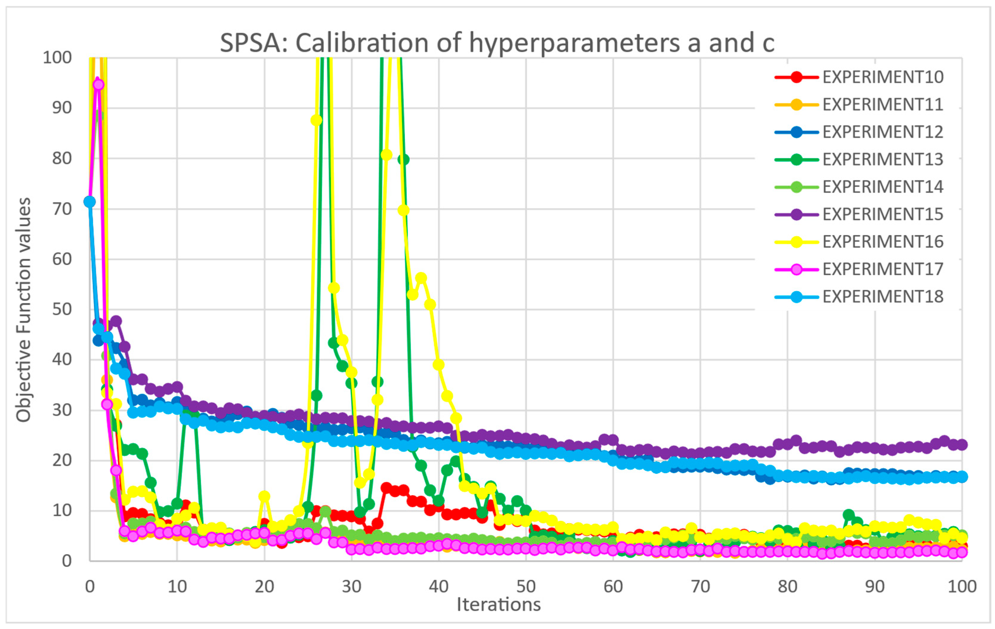
In the second set of tests, a has been tested for the values 0.001, 0.005, and 0.010, and c has been tested for the values 0.100, 0.150, and 0.200.
Figure A2 below shows the result of the second calibration step of the SPSA algorithm.
As can be observed in the graph, the parameters’ configuration that presents the best performance is a = 0.005 and c = 0.100. With the described setup, the objective function, which is equal to 71.431 at the iteration 0, decreases down to 1.788 at the iteration 100, even though the best solution, equal to 1.523, is found at the iteration 88.
Figure A2. Second step of SPSA hyperparameters’ calibration.
Futuretransp 05 00118 g0a2

Appendix A.1.2. Calibration of the PSO Algorithm

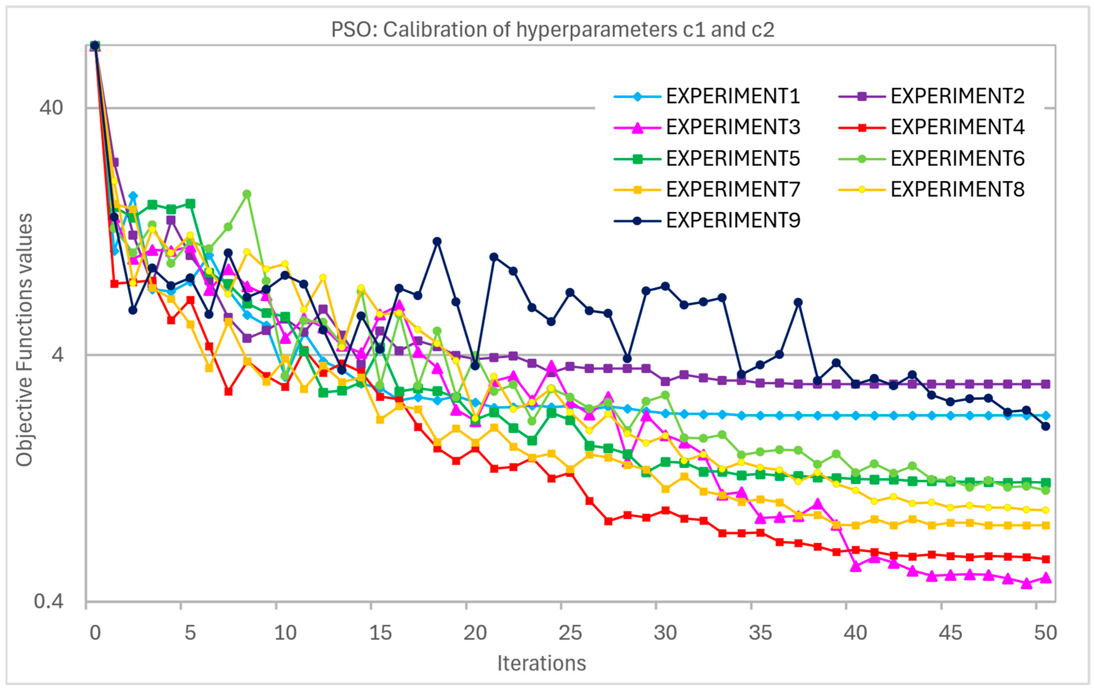
The calibration of the SPSA algorithm has been performed by setting the maximum number of iterations to 50 and with regard to two parameters, c1 and c2. For both the parameters, the values tested are 0.5, 1.5, and 2.5 for a total of nine tests.
Figure A3 below shows the result of the calibration of the PSO algorithm.
Figure A3. PSO hyperparameters’ calibration.
Futuretransp 05 00118 g0a3
As can be observed in the graph above, the parameters’ configuration that presents the best performance is c1 = 0.5 and c2 = 2.5. With the described setup, the objective function decreases down to 0.504 at the final iteration 50, even though the best solution, equal to 0.478, is found at iteration 49.
Table A2 below reports the obtained values of the objective functions obtained for the different combination of the values of the parameters c1 and c2. For the further execution of the calibration experiments, however, the configuration with c1 = c2 = 0.5 has been used. This choice is motivated by the intention to avoid constraining the algorithm toward a potentially sub-optimal local minimum, thereby favoring a broader exploration of the solution space. Exploration is preferred to exploitation.
Table A2. PSO hyperparameters’ calibration results.
c2
c10.51.52.5
0.52.2783.0450.478
1.50.5981.2171.135
2.50.8170.9402.055

Appendix A.1.3. Calibration of the ADAM Algorithm

The calibration of the ADAM algorithm has been performed by setting the maximum number of iterations to 50 and with regard to two parameters, alpha and eps_grad. For both the parameters, the values tested are 0.5, 1.5, and 2.5 for a total of nine tests.
Figure A4 below shows the result of the second calibration step of the ADAM algorithm.
Figure A4. ADAM hyperparameters’ calibration.
Futuretransp 05 00118 g0a4
As can be observed in the graph above, the parameters’ configuration that presents the best performance is eps_grad = 0.01 and alpha = 0.15. With the described setup, the objective function decreases down to 1.169 at the final iteration 50, even though the best solution, equal to 0.894, is found at iteration 48. Table A3 below reports the obtained values of the objective functions obtained for the different combinations of the values for the parameters alpha and eps_grad.
Table A3. ADAM hyperparameters’ calibration results.
Alpha
Eps_grad0.050.10.15
0.00124.3738.2336.185
0.018.7562.1100.894
0.14.6191.1200.941

Appendix A.2. Analysis of the Goodness-of-Fit Functions

The most widely used GoF function is the quadratic error (SE). Like other estimators, such as RMSE and U, SE uses the squared difference between simulated and observed measurements to assess the goodness-of-fit. Low GoF values indicate a good fit; however, this GoF strongly penalizes large errors. SE is the basis of the famous least squares method, provides the best parameter estimation for linear models with zero mean errors, and is unaffected by systematic (unbiased) and uncorrelated errors. However, there is no obvious reason to prefer SE to other measures of GoF, such as RMSE, as an objective function for a transport simulation model calibration problem because such models are generally nonlinear.
Using the tests performed to calibrate the three optimization algorithms’ hyperparameters, having used the squared error as the goodness-of fit method, several goodness-of fit values have been calculated and their behavior analyzed.
Reported below are the equations of each listed goodness-of fit formulation. In all the following expressions, x and y represent, respectively, the simulated and observed measurements (Msim, Mobs) used in the calibration problem, while N represents the total amount of data available considering all possible dimensions, spatial, temporal, etc. and i represents the generic single observation. In addition, x, σx, y, and σy represent the mean and standard deviation of the simulated and observed data, respectively.
Squared Error   SE x , y = i = 1 N x i y i 2
Mean Normalized Error   MNE x , y = 1 N i = 1 N x i y i y i
Mean Absolute Error   MAE x , y = 1 N i = 1 N x i y i
Mean Absolute Normalized Error   MANE x , y = 1 N i = 1 N x i y i y i
Mean Absolute Percentage Error   MAPE x , y = 100 % N i = 1 N x i y i y i
Weighted Absolute Percentage Error   WAPE x , y = 100 % i = 1 N x i y i i = 1 N y i
Root Mean Square Error   RMSE x , y = 1 N i = 1 N x i y i 2 2
Root Mean Squared Normalized Error   RMSNE x , y = 1 N i = 1 N x i y i y i 2 2
The Geoffrey E . Havers statistic   GEH x , y = i = 1 N 2 x i y i 2 x i + y i 2
Correlation Coefficient   r x , y = 1 N 1 i = 1 N x i x ¯ i y i y ¯ i σ x σ y
Some observations are summarized below.
  • MNE is useful for indicating the presence of systematic bias, but not for use in calibration because low values of the objective function do not ensure a good fit.
  • MAE is among the most suitable goodness-of-fit tests.
  • MANE shows limits particularly when there are low non-zero values in the data.
  • MAPE is an intuitive percentage-based formulation, which makes it attractive for communicating calibration quality to non-technical stakeholders. However, its reliability can be compromised when observed values are near zero, leading to disproportionately large errors or undefined results.
  • WAPE addresses the limitation showed by MAPE and is often used as a complementary or alternative metric. WAPE scales the total absolute error by the sum of observed values, offering greater robustness in datasets that include low-demand segments.
  • RMSE is commonly used, sensitive to high errors, and aligned with the least squares model method. It is sensitive to outliers and gives no indication of systematic errors.
  • RMSNE shows limits particularly when there are low non-zero values in the data.
  • GEH is often used in traffic simulation calibration problems. The direct minimization of summed GEH is a useful component in multi-objective optimization due to its nonlinear scaling.
  • r is widely used and useful in linear problems. It is not suitable for nonlinear problems, penalized by outliers, and does not control overfitting.
As discussed in the previous paragraph, during the algorithms’ hyperparameters calibration stage, a set of tests have been performed.
Specifically, the SPSA has regarded 18 tests each made of 100 iterations for a total of 1800 objective function evaluations. The PSO has regarded 9 tests each made of 50 iterations for a total of 9000 objective function evaluations, and the ADAM has regarded 9 tests each made of 50 iterations for a total of 450 objective function evaluations.
For each objective function evaluation (SE), the above-described potential goodness-of-fit has been evaluated. Moreover, the distance between the current solution and the true solution, which is known (refer to Table A1), has also been evaluated. This distance is defined as the square root of the squared error between the Beta-current and the Beta-true vectors.
The relative trend of each goodness-of-fit test across the iterations is well represented by the graph in Figure A5 in which the results of SPSA calibration experiment 1 are reported (the other graphs present a similar trend).
By analyzing Figure A5 below, the following considerations can be made.
  • SE has the greatest reduction, as this is the objective function to be minimized.
  • RMSNE and MNE present a very limited relative reduction.
  • MANE/MAPE presents a stable trend but not a high decrease.
  • GEH presents a more fluctuating trend and a decrease.
  • WAPE and RMSE present a stable trend similar to the SE trend and the highest decrease, except the SE trend, which is the defined objective function.
Finally, for each test, the correlation coefficient between each GoF and the distance between the solution–true solution is calculated.
Figure A5. Relative trend of goodness-of-fit estimated during SPSA experiment 1.
Futuretransp 05 00118 g0a5
Table A4, Table A5, and Table A6 report the results for each algorithm, SPSA, PSO, and ADAM, respectively, illustrating the average correlation coefficient across the different tests.
Table A4. Analysis of SPSA results.
GoFCorrelation
RMSE0.878
GEH0.872
MAE0.862
WAPE0.862
MAPE0.861
MANE0.861
Correlation r0.844
SE0.837
RMSNE0.609
MNE−0.205
Table A5. Analysis of PSO results.
GoFCorrelation
MANE0.741
MAPE0.741
RMSE0.733
GEH0.732
WAPE0.729
MAE0.729
SE0.617
Correlation r0.615
RMSNE0.584
MNE−0.309
Table A6. Analysis of ADAM results.
GoFCorrelation
RMSE0.788
WAPE0.783
MAE0.783
MANE0.781
MAPE0.781
Correlation r0.765
SE0.761
GEH0.720
RMSNE0.598
MNE−0.299
By analyzing the tables above, the following considerations can be obtained. The MNE presents a negative correlation with the distance (between the solutions—and the true solution), indicating that MNE is not suitable to be used as a GoF. The RMSNE and SE present the worst performances. Different GoF tests perform differently with different algorithms, such as GEH and the correlation coefficient. MAE, MANE, MAPE, and WAPE rank in the middle to highly. The RMSE is always in the first three positions.

Appendix A.3. Experimental Design

Two sets of different experiments have been defined to test the performances and effectiveness of the designed model and algorithms.
Specifically, the first set of experiments has been produced by assigning random values to the set of parameters subject to the calibration problem, similarly to what has been completed for the hyperparameter calibration.
Table A7 reported below shows the values randomly assigned to the 16 parameter multipliers which lead to the experiments 1, 2, and 3.
Table A7. Random values assigned to parameters multipliers in experiments 1, 2, and 3.
Parameter MultipliersExperiment 1Experiment 2Experiment 3
BETA_TT1.2961.3631.647
BETA_WALK0.8071.8870.500
BETA_TRANSFER1.7890.7881.161
LAMBDA_APP0.4720.9400.457
LAMBDA_EMP0.8710.2990.302
LAMBDA_EOP0.5850.7340.350
LAMBDA_NEMP0.6610.9630.323
LAMBDA_NEOP0.8830.9460.291
LAMBDA_PRIMPUPIL0.8030.9680.750
LAMBDA_RPLUSMP0.7990.5420.737
LAMBDA_RPLUSOP0.6850.4300.633
LAMBDA_RMP0.9330.5230.853
LAMBDA_ROP0.5150.4960.599
LAMBDA_SECPUPIL0.8540.9310.438
LAMBDA_UNISTMP0.5700.8370.994
LAMBDA_UNISTOP0.6130.6130.611
For the first set of three experiments, the objective function values—defined as 1000× SE—are as follows: 23.166, 138.483, and 154.320, respectively.
A second set of experiments was generated by directly assigning random values to the observed measurement set, resulting in three additional calibration scenarios. In particular, random perturbations were applied to the initial attractiveness values of the zones: ±10% for experiment 4, ±25% for experiment 5, and ±50% for experiment 6. These modified values were subsequently normalized so that their total summed to 100%.
Table A8 reported below shows the values randomly assigned to the 49 zones’ attractiveness which led to the experiments 4, 5, and 6.
Table A8. Values of zones’ attractiveness randomly assigned to zones in experiments 4, 5, and 6.
Zone No.Initial ValuesExperiment 4Experiment 5Experiment 6
20151.65101.85291.46951.3000
25178.89878.04276.67457.9803
25184.60504.71095.61852.5181
25192.39572.26042.34801.7292
25200.47910.50910.44560.7702
25210.04700.05130.05690.0668
25222.81442.51572.98353.9090
25260.70940.63410.69530.9775
25280.16270.15030.16110.2331
25412.80482.86933.25383.1595
25422.50382.53652.60412.6835
25441.42651.27511.78330.7800
25457.03747.54878.65668.8509
25511.89021.99001.55011.0336
25521.03551.04900.95271.6534
25531.60211.62301.87461.4543
25541.31011.22310.98261.3755
25551.68061.51891.42861.6174
25560.44830.43630.41700.2451
25571.44391.54881.19851.2001
25584.40954.33574.58623.2793
25822.69352.67522.42432.3271
25835.50026.00915.33565.8950
25841.64901.58861.63261.2985
25851.47411.59581.69531.4832
25862.70832.47472.84392.5473
25871.33131.44121.10511.6307
25882.09091.99361.75651.2577
25971.17831.28730.91911.9201
26230.03600.03650.03460.0472
27632.24272.38342.37743.1640
27641.03230.98430.91881.3773
27653.48593.60074.14852.0205
27661.58791.41941.47692.4139
27673.02353.09302.29803.5381
27680.94740.85630.72011.1501
27691.40211.50401.16381.0734
27701.20331.12341.26361.9082
27711.06441.01491.09641.5249
27722.69802.89402.56333.2752
27731.46571.42661.42181.7633
27741.35581.45431.46440.9193
27751.59571.58481.40432.2861
27760.77760.71820.81650.4592
27772.73732.60992.84702.4248
27820.29200.27840.35330.4535
27870.86440.84131.00280.6996
27890.00000.00000.00000.0000
39184.20694.42905.17494.3248
In this second set of experiments, the scale factor used in the objective function was adjusted to ensure that the resulting values remained within the range of 20 to 200. Specifically, the objective function was defined as 100× SE for experiment 4, 10× SE for experiment 5, and 1× SE for experiment 6. These modifications were made to maintain consistency and comparability across experiments with differing levels of perturbation.
The corresponding objective function values obtained from these experiments are 183.067 for experiment 4, 120.214 for experiment 5, and 21.563 for experiment 6.
As the scaling factor in the objective function has been modified with respect to the hyperparameters’ calibration tests, some algorithms’ settings have also been slightly modified.

References

  1. Park, B.; Qi, H. Development and Evaluation of a Procedure for the Calibration of Simulation Models. Transp. Res. Rec. J. Transp. Res. Board 2005, 1934, 208–217. [Google Scholar] [CrossRef]
  2. Dowling, R.; Skabardonis, A.; Alexiadis, V. Traffic Analysis Toolbox, Volume III: Guidelines for Applying Traffic Microsimulation Modeling Software; Report No. FHWA-HRT-04-040; Federal Highway Administration: Washington, DC, USA, 2004.
  3. U.K. Department for Transport. TAG UNIT M2.1: Variable Demand Modelling. Available online: https://assets.publishing.service.gov.uk/government/uploads/system/uploads/attachment_data/file/934979/tag-m2-1-variable-demand-modelling.pdf (accessed on 5 November 2020).
  4. Ciuffo, B.; Punzo, V.; Montanino, M. The Calibration of Traffic Simulation Models: Report on the Assessment of Different Goodness of Fit Measures and Optimization Algorithms; JRC Scientific Reports, JRC68403; Publications Office of the European Union: Luxembourg, 2012; pp. 13–19. [Google Scholar]
  5. Cascetta, E.; Russo, F. Calibrating Aggregate Travel Demand Models with Traffic Counts: Estimators and Statistical Performance. Transportation 1997, 24, 271–293. [Google Scholar] [CrossRef]
  6. Shafiei, E.; Heydari, M.; Abbaspour, A. Calibration of Traffic Simulation Models Using Evolutionary Algorithms. Transp. Res. Part C 2018, 92, 456–479. [Google Scholar]
  7. Ben-Akiva, M.; Bierlaire, M.; Koutsopoulos, H.N.; Mishalani, R. DynaMIT: Simulation-Based Dynamic Traffic Assignment and Travel Forecasting. Transp. Rev. 2012, 32, 113–147. [Google Scholar]
  8. Fusco, G.; Colombaroni, C.; Gemma, A.; Lo Sardo, S. A Quasi-Dynamic Traffic Assignment Model for Large Congested Urban Road Networks. Int. J. Math. Models Methods Appl. Sci. 2013, 7, 341–349. [Google Scholar]
  9. Qin, X.; Mahmassani, H.S. Adaptive Calibration of Dynamic Speed-Density Relations for Online Network Traffic Estimation and Prediction Applications. Transp. Res. Rec. 2004, 1876, 82–89. [Google Scholar] [CrossRef]
  10. Hou, T.; Mahmassani, H.S.; Alfelor, R.M.; Kim, J.; Saberi, M. Calibration of Traffic Flow Models under Adverse Weather and Application in Mesoscopic Network Simulation. Transp. Res. Rec. 2013, 2391, 92–104. [Google Scholar] [CrossRef]
  11. Vaze, V.; Antoniou, C.; Wen, Y.; Ben-Akiva, M. Calibration of Dynamic Traffic Assignment Models with Point-to-Point Traffic Surveillance. Transp. Res. Rec. J. Transp. Res. Board 2009, 2090, 1–9. [Google Scholar] [CrossRef]
  12. Zheng, F.; Van Zuylen, H. The Development and Calibration of a Model for Urban Travel Time Distributions. J. Intell. Transp. Syst. 2014, 18, 81–94. [Google Scholar] [CrossRef]
  13. Antoniou, C.; Azevedo, C.L.; Lu, L.; Pereira, F.; Ben-Akiva, M. W-SPSA in Practice: Approximation of Weight Matrices and Calibration of Traffic Simulation Models. Transp. Res. Part C Emerg. Technol. 2015, 59, 129–146. [Google Scholar] [CrossRef]
  14. Liu, F.; Bellemans, T.; Janssens, D.; Wets, G.; Adnan, M. A Methodological Approach for Enriching Activity–Travel Schedules with In-Home Activities. Sustainability 2024, 16, 10086. [Google Scholar] [CrossRef]
  15. Wang, D.; Liao, F. Formulation and Solution for Calibrating Boundedly Rational Activity-Travel Assignment: An Exploratory Study. Commun. Transp. Res. 2023, 3, 100092. [Google Scholar] [CrossRef]
  16. Poole, A.; Kotsialos, A. Swarm Intelligence Algorithms for Macroscopic Traffic Flow Model Validation with Automatic Assignment of Fundamental Diagrams. Appl. Soft Comput. 2016, 38, 134–150. [Google Scholar] [CrossRef]
  17. Tavassoli, A.; Mesbah, M.; Hickman, M. Calibrating a Transit Assignment Model Using Smart Card Data in a Large-Scale Multi-Modal Transit Network. Transportation 2020, 47, 2133–2156. [Google Scholar] [CrossRef]
  18. Colombaroni, C.; Fusco, G.; Isaenko, N. Meta-heuristic aggregate calibration of transport models exploiting data collected in mobility. Case Stud. Transp. Policy 2023, 13, 101039. [Google Scholar] [CrossRef]
  19. Larijani, A.N.; Olteanu-Raimond, A.-M.; Perret, J.; Brédif, M.; Ziemlicki, C. Investigating Mobile Phone Data to Estimate Origin–Destination Flows in the Paris Region: A Microscopic, Individual-Based Approach to Infer Transportation Modes. Transp. Res. Procedia 2015, 6, 64–78. [Google Scholar] [CrossRef]
  20. Nahmias-Biran, B.; Cohen, S.; Simon, V.; Feldman, I. Large-Scale Mobile-Based Analysis for National Travel Demand Modeling. ISPRS Int. J. Geo-Inf. 2023, 12, 369. [Google Scholar] [CrossRef]
  21. Mauricio, L. Fundamental Understanding of Mobile Phone Data for Transport Applications. I-Manag. S J. Mob. Appl. Technol. 2024, 11, 1–12. [Google Scholar]
  22. Ben-Akiva, M. Estimation of Travel Demand Parameters from Macroscopic Flows. Transp. Sci. 1985, 19, 15–32. [Google Scholar]
  23. Transportation Planning Software 2024, PTV VISUM 24; PTV AG: Karlsruhe, Germany, 2024.
  24. Spall, J.C. Stochastic Approximation: A New Adaptive Algorithm for Noisy Systems. IEEE Trans. Autom. Control 1998, 43, 7–12. [Google Scholar]
  25. Kennedy, J.; Eberhart, R. Particle Swarm Optimization. In Proceedings of the International Conference on Neural Networks (ICNN’95), Perth, WA, Australia, 27 November–1 December 1995; Volume 4, pp. 1942–1948. [Google Scholar]
  26. Kingma, D.P.; Ba, J. Adam: A Method for Stochastic Optimization. In Proceedings of the International Conference on Learning Representations, Banff, AB, Canada, 14–16 April 2014. Poster 1–15. [Google Scholar]
  27. Plackett, R.L. Some Theorems in Least Squares. Biometrika 1950, 37, 149–157. [Google Scholar] [CrossRef] [PubMed]
Figure 1. Representation of the test network used in this research task.
Futuretransp 05 00118 g001
Figure 2. Trend of the objective function value over model runs for the three calibration algorithms—experiment 1.
Futuretransp 05 00118 g002
Figure 3. Trend of the objective function value over model runs for the three calibration algorithms—experiment 2.
Futuretransp 05 00118 g003
Figure 4. Trend of the objective function value over model runs for the three calibration algorithms—experiment 3.
Futuretransp 05 00118 g004
Figure 5. Trend of the objective function value over model runs for the three calibration algorithms—experiment 4.
Futuretransp 05 00118 g005
Figure 6. Trend of the objective function value over model runs for the three calibration algorithms—experiment 5.
Futuretransp 05 00118 g006
Figure 7. Trend of the objective function value over model runs for the three calibration algorithms—experiment 6.
Futuretransp 05 00118 g007
Figure 8. Trend of the objective function normalized value over model runs for the three calibration algorithms—average over all six experiments.
Futuretransp 05 00118 g008
Table 1. Experiment 1—key observations of algorithms’ performances.
METRICSPSAPSOADAM
Best final objective value
Smooth convergence
Fast early improvements
Noise in trajectoryHighLowModerate
Long-term improvement
Table 2. Experiment 1—algorithm results: objective function and other KPI minimum values.
KPIINITIALSPSAPSOADAM
Objective Function23.1661.3651.8331.239
SE0.0230.0010.0020.001
MNE0.0190.0180.0080.017
MAE0.0160.0040.0050.004
MANE0.0320.0240.0250.024
MAPE3.2182.3732.4562.359
WAPE0.7780.1910.2280.182
RMSE0.0220.0050.0060.005
RMSNE0.1440.1430.1430.143
GEH0.0430.0100.1870.147
Correlation Coefficient1.0001.0000.9991.000
Distance solution—true solution1.4550.9670.9720.733
Correlation solution—true solutionN/A0.6830.6890.816
Table 3. Experiment 1—algorithms’ parameter recovery performance.
ParametersSPSAPSOADAMTrue Value
BETA_TravelTime1.2751.2561.2811.281
BETA_WALK0.7770.7650.7730.807
BETA_TRANSFER1.1421.2611.4641.789
LAMBDA_APP0.8250.9210.7710.472
LAMBDA_EMP0.8350.9340.8800.871
LAMBDA_EOP0.5710.5990.6030.585
LAMBDA_NEMP0.8170.7210.8540.661
LAMBDA_NEOP0.7720.5150.7240.883
LAMBDA_PRIMPUPIL0.7250.7430.7840.803
LAMBDA_RPLUSMP0.7990.9360.9150.799
LAMBDA_RPLUSOP0.8440.9270.6490.685
LAMBDA_RMP0.9010.9880.4530.933
LAMBDA_ROP0.7590.5610.5630.515
LAMBDA_SECPUPIL0.8460.8481.0000.854
LAMBDA_UNISTMP0.9490.2510.6550.570
LAMBDA_UNISTOP0.9550.2500.6290.613
Table 4. Experiment 2—key observations of algorithms’ performances.
METRICSPSAPSOADAM
Best final objective value
Smooth convergence
Fast early improvements
Noise in trajectoryHighLowModerate
Long-term improvement
Table 5. Experiment 2—algorithm results: objective function and other KPI minimum values.
KPIINITIALSPSAPSOADAM
Objective Function138.4833.2491.9902.485
SE0.1380.0030.0020.002
MNE0.0190.0170.0120.016
MAE0.0330.0060.0050.005
MANE0.0370.0250.0240.025
MAPE3.7192.4672.3632.512
WAPE1.6170.2890.2320.267
RMSE0.0530.0080.0060.007
RMSNE0.1450.1430.1430.143
GEH0.0840.0130.1850.017
Correlation Coefficient1.0001.0001.0001.000
Distance solution—true solution1.6531.2011.5081.334
Correlation solution—true solutionN/A0.7040.6490.654
Table 6. Experiment 2—algorithms’ parameter recovery performance.
ParametersSPSAPSOADAMTrue Value
BETA_TravelTime1.405 1.365 1.177 1.363
BETA_WALK1.784 2.000 2.000 1.887
BETA_TRANSFER0.677 1.651 1.451 0.788
LAMBDA_APP0.999 0.348 0.616 0.940
LAMBDA_EMP0.267 0.393 0.507 0.299
LAMBDA_EOP0.698 0.695 1.000 0.734
LAMBDA_NEMP0.976 1.000 0.494 0.963
LAMBDA_NEOP0.990 0.875 0.925 0.946
LAMBDA_PRIMPUPIL0.466 0.606 0.250 0.968
LAMBDA_RPLUSMP0.866 0.283 0.893 0.542
LAMBDA_RPLUSOP0.951 1.000 0.397 0.430
LAMBDA_RMP0.541 1.000 0.682 0.523
LAMBDA_ROP0.964 0.406 0.663 0.496
LAMBDA_SECPUPIL0.368 0.746 0.694 0.931
LAMBDA_UNISTMP0.422 0.250 0.997 0.837
LAMBDA_UNISTOP0.344 0.503 0.892 0.613
Table 7. Experiment 3—key observations of algorithms’ performances.
METRICSPSAPSOADAM
Best final objective value
Smooth convergence
Fast early improvements
Noise in trajectoryHighLowModerate
Long-term improvement
Table 8. Experiment 3—algorithm results: objective function and other KPI minimum values.
KPIINITIALSPSAPSOADAM
Objective Function154.3201.2171.2379.469
SE0.1540.0010.0010.009
MNE0.0180.0180.0130.018
MAE0.0420.0040.0040.010
MANE0.0490.0230.0230.028
MAPE4.8612.3102.3302.765
WAPE2.0800.1770.1900.512
RMSE0.0560.0050.0050.014
RMSNE0.1480.1430.1430.143
GEH0.1110.0090.1510.024
Correlation Coefficient0.9990.9990.9990.999
Distance solution—true solution1.9430.6750.6491.603
Correlation solution—true solutionN/A0.8910.8910.341
Table 9. Experiment 3—algorithms’ parameter recovery performance.
ParametersSPSAPSOADAMTrue Value
BETA_TravelTime1.628 1.674 1.333 1.647
BETA_WALK0.500 0.500 0.500 0.500
BETA_TRANSFER1.091 1.068 0.817 1.161
LAMBDA_APP0.858 0.268 0.348 0.457
LAMBDA_EMP0.332 0.271 0.382 0.302
LAMBDA_EOP0.367 0.343 1.000 0.350
LAMBDA_NEMP0.306 0.374 1.000 0.323
LAMBDA_NEOP0.353 0.484 0.656 0.291
LAMBDA_PRIMPUPIL0.760 0.711 0.927 0.750
LAMBDA_RPLUSMP0.391 0.883 0.381 0.737
LAMBDA_RPLUSOP0.794 0.578 0.250 0.633
LAMBDA_RMP0.849 0.463 0.327 0.853
LAMBDA_ROP0.714 0.811 0.740 0.599
LAMBDA_SECPUPIL0.621 0.665 0.250 0.438
LAMBDA_UNISTMP0.946 0.761 0.250 0.994
LAMBDA_UNISTOP0.909 0.692 0.250 0.611
Table 10. Experiment 4—key observations of algorithms’ performances.
METRICSPSAPSOADAM
Best final objective value
Smooth convergence
Fast early improvements
Noise in trajectoryHighLowModerate
Long-term improvement
Table 11. Experiment 4—algorithm results: objective function and other KPI minimum values.
KPIINITIALSPSAPSOADAM
Objective Function183.067118.381123.445130.858
SE1.8311.1841.2341.309
MNE0.0120.0020.0030.001
MAE0.1220.1050.1070.108
MANE0.0790.0760.0750.075
MAPE7.9077.6107.5377.507
WAPE5.9675.1495.2675.295
RMSE0.1930.1550.1590.163
RMSNE0.1580.1570.1570.157
GEH0.2940.2013.4860.205
Correlation Coefficient0.9940.9940.9910.994
Table 12. Experiment 5—key observations of algorithms’ performances.
METRICSPSAPSOADAM
Best final objective value
Smooth convergence
Fast early improvements
Noise in trajectoryHighLowModerate
Long-term improvement
Table 13. Experiment 5—algorithm results: objective function and other KPI minimum values.
KPIINITIALSPSAPSOADAM
Objective Function120.214100.562101.430100.493
SE12.02110.05610.14310.049
MNE−0.011−0.031−0.022−0.024
MAE0.2790.2700.2680.271
MANE0.1450.1440.1450.144
MAPE14.47414.40114.46814.416
WAPE13.67713.23813.11613.265
RMSE0.4950.4500.4550.453
RMSNE0.2100.2100.2110.209
GEH0.7970.5928.0640.596
Correlation Coefficient0.9610.9610.9560.961
Table 14. Experiment 6—key observations of algorithms’ performances.
METRICSPSAPSOADAM
Best final objective value
Smooth convergence
Fast early improvements
Noise in trajectoryHighLowModerate
Long-term improvement
Table 15. Experiment 6—algorithm results: objective function and other KPI minimum values.
KPIINITIALSPSAPSOADAM
Objective Function21.56320.20120.18820.371
SE21.56320.20120.18820.371
MNE−0.028−0.042−0.044−0.042
MAE0.4920.4760.4740.477
MANE0.3190.3110.3100.313
MAPE31.86931.05730.95231.338
WAPE24.10323.34023.24223.370
RMSE0.6630.6420.6420.645
RMSNE0.4000.3940.3930.396
GEH1.1061.05516.3531.071
Correlation Coefficient0.9280.9280.9230.928
Table 16. Key overall observations of algorithms’ performances.
METRICSPSAPSOADAM
Best final objective value±±±
Smooth convergence
Fast early improvements
Noise in trajectoryHighLowModerate
Long-term improvement
Disclaimer/Publisher’s Note: The statements, opinions and data contained in all publications are solely those of the individual author(s) and contributor(s) and not of MDPI and/or the editor(s). MDPI and/or the editor(s) disclaim responsibility for any injury to people or property resulting from any ideas, methods, instructions or products referred to in the content.