Model-Based Bikeability Indexing for Inter-City Comparisons to Evaluate Infrastructure and Level of Service for Cyclists

Abstract

“Bikeability” is a measure of a city’s suitability for a bicycle-based lifestyle. Cities are striving to increase the number of cyclists in their traffic to decrease congestion and increase sustainability. Bikeability is therefore a relevant metric to measure a city’s progress towards this goal. This study is an application of a previously developed programmatic bikeability model. It is used to calculate bikeability for eight different cities in order to compare their bikeability indices. It was found that the bikeability between different cities is more similar than their modal share would suggest. This correlates more strongly with different metrics for measuring city infrastructure quality than with existing studies regarding bikeability. For this reason, this bikeability model is not suited as a replacement for existing indices but has to be evaluated separately. This revealed a disparity between the availability of urban infrastructure, the level of satisfaction with said infrastructure and its statistical use. Possible solutions and options to further develop the model were discussed.

1. Introduction

As cities fight congestion, many of them look towards alternatives to car-centric urban planning. In addition to public transportation, the bicycle is a popular choice among these alternatives, as it is an established, low-cost form of mobility that is inherently sustainable. At the same time, increased health awareness among the population, as well as a lower athletic hurdle for cycling due to the popularization of pedelecs, are increasingly bringing cycling into the focus of urban planners. This leads to a slow change in the bicycle’s image from a form of leisurely activity to a serious form of transportation [1]. To encourage more citizens to switch from cars to bicycles for their daily journeys, cities are investing more in cycling infrastructure. Countries such as Denmark and the Netherlands are pioneers in bicycle-orientated urban planning. However, most cities are reluctant to embrace such transformation processes. One reason for this is the high degree of overview of the existing urban topology, which would be required for the bicycle-friendly conversion of the transport network.

To identify the pent-up demand, the potential, and also the qualities in the existing bicycle infrastructure, research projects and inventories are being carried out in many cities. The collection and initial categorization of infrastructure data usually accounts for a large part of the time required for local research projects on bikeability.

In a soon-to-be published paper, a model using open data was developed to automatically calculate bikeability [2]. This initial paper includes an application of the model for two different cities. However, a broader application of the model is needed to develop its potential. The goal of this study is to provide that broader application while also evaluating the possibility of using bikeability as a point of comparison between different cities. In this process, the method was further developed and the caveats of its application explored. To verify the results, a variety of recent studies in neighboring fields were consulted.

The term “bikeability” has been used in different ways over the years with no single, commonly used definition. As this study aims to compare the bikeability of different cities, it is necessary to first make sure the term is clearly defined. A clear explanation of bikeability is given in [3]:

’Bikeability: An assessment of an entire bikeway network for perceived comfort and convenience and access to important destinations’.

The “important destinations” mentioned in the definition are often referred to as “Points of Interest” (POIs). This definition is used in contrast to two related topics, which are often conflated with bikeability: these topics are “bicycle suitability” and “bicycle friendliness”. Bicycle suitability is a more limited metric that is specific to one part of a city’s road network at a time. Usually, suitability analysis includes evaluations on the quality of a road’s bicycle paths, using metrics such as its separation from the road and its surface area. An evaluation of suitability is a necessary step in the calculation of bikeability, as discussed in Section 3.1. Meanwhile, bicycle friendliness is a much broader measure, including local culture and attitude towards cycling as much as the available infrastructure. Surveys of the happiness of cyclists are generally a common measure of bicycle friendliness. Some of these surveys, as well as previous reports on bicycle suitability, are used as references in this study. These surveys are listed in Section 4.1. All other references used in the development of this study are listed in Section 2.

2. Literature Review

Aside from the 2012 study by Lowry et al. [3], which is used to define the term in Section 1, there are other studies that inform the theoretical background of bikeability calculations.

Influential studies on bikeability include the work of Winters et al. in their 2013 [4] and 2016 [5] studies, as well as a 2012 study by Titze et al. [6].

Many previous studies on the relative or specific bikeability of cities exist. Some of them are listed here:

• The bikeability of Dresden, which is also discussed in this study, has already been evaluated by a 2017 thesis [7]. This is a direct application of the model developed by Winters et al. [4].
• The bikeability of Munich has previously been evaluated, although the study is more concerned with bicycle suitability [8].
• A 2021 dissertation has calculated bikeability for Berlin and Athens [9].

The “Bikeability and Walkability Evaluation Table” by Hoedl et al. [10] offers a further approach for quantifying the influence of infrastructure on bikeability.

As the bikeability model described in this paper and discussed in Section 3.1 uses pathfinding, research was gathered on algorithms previously used. The algorithm used in the model most closely resembles the one described in a 2014 paper by Halldorsdottir et al. [11]. However, many different approaches exist, including the ones described by Owais and Alshehri in 2020 [12] and by Almutairi and Owais in 2025 [13].

The impact of different types of measures to improve bikeability has been quantified for the city of Copenhagen. This research has been published in two papers by Fosgerau et al. [14,15].

In addition to scientific studies, there are also public reports on the success of measures to improve bikeability. These include the Dutch “Fietsbalans” studies [16], the Danish National Travel Surveys [17] and the German series of studies “Mobilität in Deutschland” [18]. The latter is discussed in more detail in Section 4.1.

Private research into the topic of bikeability includes the Copenhagenize Index [19], the Bicycle Cities Index [20] and the “Fahrradklima-Test” [21], all of which are discussed in Section 4.1.

The key difference between the previous study and this one is the high degree of automation and the entirely open data-based approach, leading to increased transparency and reproducibility.

3. Methods

The purpose of this study is to compare the bikeability of several German cities. This comparison is used to quantify the state of development of the bicycle infrastructure in different cities and to evaluate the model for calculating the bikeability introduced in [2]. This model is thoroughly explained in Section 3.1 by applying it to different cities and working with it to gather scientific insights. To enable the comparison, the following steps were taken:

• Several German cities were selected for the subsequent comparison. The criteria for this selection were representativeness, ambition to expand urban cycling and availability of data. In addition, a selection of non-German comparison cities was performed, which were included in the comparison as examples.
• A bikeability calculation was carried out for each of these cities.
• The resulting geographical bikeability data was filtered and sampled to ensure comparability (see Section 3.4). The individual urban topological conditions of the sample cities were taken into account. The purpose of these calculations was to establish comparability of the individual values.
• The results of this calculation were overlaid with existing data to verify the validity of the calculation model. These data include surveys on the quality of cycling in the cities concerned, existing infrastructure analyzes and data on the modal split of cyclists in traffic (See Section 5).

3.1. Bikeability Calculation Algorithm

The Bikeability model used in this study was extensively described in German in [2], which is expected to be released in May.

All data gathered for this article are publicly available via Zenodo [22]. The code is also available on Github [23].

All of the context necessary to understand the model is given in the following section.

All data used in the bikeability calculation for this study are sourced from OSM [24]. OSM has previously been proven to be a reliable source for bicycle infrastructure data [25]. Geographical OSM data for a specified city is downloaded and processed, primarily using functionality provided by the python package OSMnx [26].

Bikeability is calculated in two steps. First, a map of the city’s infrastructure network is downloaded. Each path that theoretically allows for bicycle traffic is then assessed for the separation of biking facilities from other traffic, primarily cars. It is also evaluated for the smoothness and quality of its surface area and whether or not it is lit at night. The resulting network is then used for a path-finding algorithm that makes up the second step in the bikeability calculation. The model also provides the option to include accident data from the German “Unfallatlas” [27], but these data are highly noisy due to its statistical nature [2], so the option is disabled for this study’s application of the model.

For the calculation’s second step, a list of POIs for the city is downloaded and grouped into categories. Examples of these categories include “doctors”, which is a category composed of all generalist or specialized doctor’s offices, or “education”, which includes schools, universities, and all other educational facilities. These categories are weighed against each other according to their importance as targets for cyclists. In addition to that, a list of all residential buildings in the city is created by filtering a list of buildings. These residential buildings form the starting point for the following steps. For each of the residential buildings, five of the closest POIs of each category are selected. Then, between each building and each of these POIs, the bikeable path is found. This pathfinding takes place using a weighted shortest-path algorithm, which was chosen for its comparatively low run time. The bicycle suitability scores that were calculated in an earlier step are used as weights. The result is a score for each of the POIs chosen for the building, which quantifies the accessibility of the POI by bike. These scores are then added to each other using the aforementioned weights, resulting in one single bikeability score for each building.

3.2. Input Parameters

The bikeability calculation requires two types of input parameters. This study uses the standard parameters that were researched for the initial study [2].

The first kind of weight that is used defines the impact of points of interest in the vicinity of the address a bikeability score is calculated for. These weights are grouped into profiles. The profile used for this study represents a family with children. It is shown in

Table 1. Weights for POIs for bikeability calculation.

Category	1st Instance	2nd Instance	3rd Instance
Educational facilities	8	4	1
Doctors’ offices	5	1	0
Entertainment	2	0	0
Pharmacies and drug stores	2	0	0
Financial services	2	0	0
Gastronomy	4	2	0
Supermarkets	8	4	1
Food shops	5	1	0
Offices	8	4	1

. POIs are grouped into categories. Each category has between one and three weight factors, representing the importance of the closest three instances of POIs in these categories. Closest in this context refers to the ease with which the POI is available by bike. For example, the closest two food shops (including butchers and greengrocers for example) are considered with weights of five and one.

The weight factors in this example were synthesized from statistical data from the Danish National Travel Surveys [17] and the German National Travel Survey [28] and extensively surveyed by city planners for the initial study [2].

The second kind of weight defines the impact of different aspects of bicycle infrastructure on the calculated bicycle suitability scores. For this study, the weight factors that were compiled for the initial study were used [2]. These weights are shown in

Table 2. Weight factors for different aspects of bicycle infrastructure.

Quality Level	Separation	Surface Quality
5	0	0
4	0.05	0.1
3	0.25	0.2
2	0.35	0.35
1	0.75	0.6
0	0.9	0.9

. In general, separation and surface quality are grouped into quality levels ranging from zero to five. Each level of quality has an associated weight. The weights represent negative modifiers to bicycle suitability. A higher level of quality is associated with a lower weight, meaning that a high level of quality, i.e., a low weight, leads to high bicycle suitability. This means that a road with perfect separation from other modes of transportation and perfect surface quality has a weight of zero for both, which leads to a bicycle suitability of one.

It is important to point out that the parameter “separation” is synthesized from several different OSM parameters. This approach was chosen in order to make the model more realistic, as a low level of separation is more impactful the heavier the traffic on the relevant street. This approach also ensures completeness in the data, because there are multiple OSM tags from which separation can be calculated. Tags that are used to calculate suitability include traffic speeds and intensity and whether a bicycle path is physically separated from the street. If a path is shared between cyclists and pedestrians, service vehicles or busses, this is also considered.

The weight factors are synthesized from several of the sources listed in Section 2. The most important ones are [9,10]. It has to be noted that any weight factor needs to conform to the availability and structure of open data.

Bicycle suitability maps are a secondary result of the bikeability calculation model and can also be used in isolation. An example of this is shown in Section 5.2.

3.3. Limitations of the Model

Because the calculation model is dependent on the public availability of data, it is inherently more limited than manual surveys. This leads to a more streamlined approach to bikeability, focusing primarily on the safety of the traffic network and the accessibility of POIs. Comfort and convenience can only be approximated by using features correlated with them. These features include surface quality and illumination of the paths.

The model is also limited by its input data.

3.4. Comparability of Cities

The main point of comparison will be the mean and average bikeability scores of every city. In order to compare the bikeability scores of cities, comparability between the cities has to be established.

One problem with the method of viewing cities is the loss of regional context. For example, residents in the outskirts of one sprawling city might live closer to the center of a smaller neighboring city than to the one of their own cities. In the bikeability calculation, POIs in the neighboring cities are lost, which artificially lowers the bikeability scores of buildings at the edges of the city area. This effect is further enhanced by the fact that alternative paths through neighboring cities are also not taken into account. This results in a band of lower bikeability scores that surrounds the cities as a result of the methods used for the calculation. Examples for this phenomenon can be seen in the examples provided in Section 5.2.

Another feature of all comparisons between cities is the varying grade of urbanization between them. This is a necessary result of the fact that a city’s borders are defined, among others, by their history, administrative necessities, regional politics and general governmental rules and regulations. The effect of urbanization on a city’s bikeability is indirect but immediately noticeable when regarding the full city maps. Bikeability is higher the denser and the more interconnected the area surrounding the address for which the bikeability score is calculated is built up. A higher density of buildings is usually correlated with a larger amount of POIs in the area, while a higher interconnectivity leads to a higher availability of routes aside from main traffic arteries, leading to a higher chance of bikeable routes being available. For these reasons, the citywide bikeability average can be highly dependent on administrative decisions, like whether smaller communities bordering the main city are designated as separated towns, suburbs or full parts of the city. Whenever a specific city’s bikeability is analyzed, this needs to be taken into account. All cities that were evaluated for this study have internally varying density, with one notable exception. Utrecht’s city borders do not include a less dense ring around the main city, which makes a full comparison with other cities misleading. However, this example is insufficient for really quantifying the phenomenon, as Utrecht is expected to have a very high bikeability even without it.

City cores as defined by a fixed area of one kilometer around the cities’ respective city halls were chosen as a supplementary comparison.

After an analysis of both of these criteria for the sample group, additional alterations were performed to increase the meaningfulness of the data. One immediate issue was the varying sample size of the city core comparison. Specifically, the defined core areas for Dresden and Munich include less than one-tenth of the residential buildings the other cities’ cores include. This is due to the special situation of both of these cities as state capitals. As a result, the area around their city halls mainly consist of administrative buildings. Both of these city cores also include historic palaces with expansive parks around them. For this reason, the city core was expanded to two kilometers for both of them.

During an initial analysis of bikeability scores, it was discovered that the cities Aachen and Münster contain a much larger percentage of rural areas in their borders than initially assumed. Due to the inherently long cycle distances between rural residences and the cities’ POIs, most bikeability scores in these areas are close to zero. In order to better compare the more urban parts of these cities with the others in the selection, an additional analysis was conducted. For this, the cities’ residential buildings were sorted by their distance to the city centers. A total of 20% of the addresses that were the farthest from their respective city centers were removed, and the analysis was repeated.

In conclusion, in order to compare the values, the initial bikeability calculations were modified in the following ways:

• The worst 10% of all scores were removed in order to account for gray bands and errors in the network model.
• The 20% of buildings that were most distant from the city center were removed in order to account for the band of low scores around the city borders that is created by the calculation models.

4. Materials

All data that were collected in order to supplement the bikeability calculation are listed in this section.

4.1. Related Data and Points of Comparison

In order to validate the bikeability calculations described in this study and to ensure the precision and validity of its comparative methods, external data are needed. Studies, surveys and databases used for this purpose are described in this section. Their methodological approaches, scope and limitations are explained. Furthermore, all other sources used to develop the method described in this study are also listed.

The most obvious point of comparison for bikeability data is the general happiness among a city’s cyclist population with their situation in the respective city’s traffic. The trend in cyclist satisfaction is regularly surveyed for each German city. The “Fahrradklima-Test” (Cycling Climate Test) [21] is conducted by the German Cyclists’ Federation (Allgemeiner Deutscher Fahrrad-Club, ADFC) and awards school grades to the cities according to the survey results. The cities are then grouped by population size and ranked. Using the definitions established in Section 1, these survey scores are not directly comparable with bikeability data as any broader survey will necessarily explore bicycle friendliness rather than bikeability. Another inherent issue with the method of surveying cyclists is connected to the relation between bikeability and general bicycle usage. Because bikeability is defined by people’s subjective conception of safety in traffic, a lower bikeability leads to a lower percentage of cyclists in traffic. This means any survey of cyclists is inherently biased away from potential cyclists that do not feel comfortable maneuvering the traffic of less bikeable cities. However, because of the broad application over all German cities and the inherent connectedness of bikeability and bicycle friendliness, it is still a useful comparison.

In addition to the more subjective metric of bicyclist happiness, there is also extensive statistical research into a city’s bicycle traffic. One of the most comprehensive studies into German traffic in general is the report “Mobilität in Deutschland” (Mobility in Germany) [18], which is regularly conducted by the Federal Ministry for Digital and Transport. The part of this study that is most relevant for this study is the research on the “modal split” in cities, which is the percentage of the total distance traveled in a city that is covered by certain modes of transport. Modal split data are usually hard to compare, because different surveys use the percentage of total travels or the percentage of people who use the mode of transport as their primary one instead. Because of this, using the same source for all German Cities discussed here is important. It is important to note the age of the data. The most recent iteration of this study is from 2017. This is before the SARS-CoV-19 pandemic started a general trend towards individual mobility and Germany lowered the cost for regular use of public transportation [29], which in turn increased its modal share. At this point, there are no comprehensive data on the effect of these policies on bicycle traffic. Modal split data are also more directly linked to bicycle friendliness than to bikeability.

International comparative data on a city level concerning bikeability on a scientific level is still rare. There is, however, a large study that is regularly conducted by the insurance provider “Luko” called the “bikeable cities index”, which compiles a number of data points concerning the bikeability of notable cities around the world [20]. These include but are not limited to the modal split, the number of accidents including cyclists, the volume of public investment in bicycle infrastructure and the quality of roads. The study is mainly compiled from public data, but its methods of calculating the resulting scores are not always transparent. It is therefore unsuitable as a scientific source, but it remains a useful point of comparison.

The last study this study uses to compare the results of the bikeability calculation with is Martin Lumiste’s “CycloRank” [30]. CycloRank uses OSM (Open Street Map) data to calculate the percentage of a city’s roads that is specifically designated for cyclists (Section 3.1 provides more details regarding OSM as a source). This includes all cycleways along roads as well as footways and bus lanes shared with cyclists as well as cycle roads. It explicitly excludes any cycleway that is not physically separated from cars as well as normal roads that passively allow bike traffic. For CycloRank, the impact of roads on the overall score is weighed to decrease the impact of recreational bicycle facilities on the outskirts of a city. Concerning the definitions given in Section 1, CycloRank is closer to a bicycle suitability calculation than a bikeability calculation because it does not explicitly consider the accessibility of POIs.

Another prominent example for comparative analysis regarding the bicycle friendliness of cities is the Copenhagenize Index [19]. The Copenhagenize Index is a regular study conducted by the consulting company Copenhagenize. It weighs selected notable cities in Europe against the Danish capital of Copenhagen, which serves as an example for quality bicycle infrastructure. For this study, it was decided not to use the Copenhagenize Index as a point of comparison because of the limited number of cities it concerns itself with.

4.2. City Selection

As this study deals with a comparison of urban bikeability, the selection of the sample of analyzed cities is an important part of the work process. This selection is important because even an automated bikeability calculation is time-consuming and the comparison between cities is labor-intensive. The final selection is primarily based on the EU mission “100 climate neutral and smart cities” [31]. The reason for this selection is the interest all of these cities express to reform their traffic in order to conform to make it more sustainable and future-proof. These plans often contain a more prominent roll of bicycle traffic, especially for commuters. This contrasts with the prominent view of the bicycle as a means of transport that is mainly used for leisure activities [1]. The German cities included in this project are Aachen, Dortmund, Dresden, Heidelberg, Leipzig, Mannheim, Munich and Münster [31].

The cities were categorized and grouped in order to ensure that the cities in the final selection were different enough for a separate analysis to be meaningful and representative of a broader trend between cities. Factors that were applied include their number of residents, their geographical location and the comparative sources listed in Section 4.1. In addition to that, it is necessary for comparative data to be accessible for each city in order to be able properly verify and explain the results of the bikeability analysis. As a result of this process, the city of Heidelberg was removed from the selection as it is significantly smaller than all other listed cities and is not included in the selected comparative literature. All other cities mentioned in the study are included in the calculation.

Germany as a whole is not considered a very bikeable country in its cities. This is reflected both in the absolute numbers of the Fahrradklima-Test [21] and the middling scores in the Bikeable Cities Index [20] that most listed cities have. For this reason, one foreign city has been added as a positive example. Utrecht has been chosen as the highest ranked city of 2022’s Bikeable Cities Index and is a consistently used positive example in bikeability discourse [19]. When using the model described in this study to compare cities across national borders, there are a number of limitations and potential problems. These are explained in detail in Section 3.1. For this reason, Utrecht is used purely as a reference, not as a subject of analysis by itself.

5. Results

After the parameters were set, a bikeability calculation was run for each selected city. The results of these calculations were then evaluated against each other as well as the selected comparative parameters described in Section 4.1. These comparative parameters were introduced in Section 4.1 and are discussed in detail in this section. Any insights gained from this process are described in this section. Any problems that hindered the analyses for this study are also listed, together with possible solutions.

5.1. Reference Values

As described in Section 4.1, multiple different studies relating to the topic of bikeability were consulted. From these, relevant points of comparison relating to bikeability were chosen. These selected values are shown in

Table 3. Table of all considered reference values for sample cities.

City	Population	Bicycle Climate [21]	Cycle Road Share [30]	Bicycle Share
Aachen	261,472 [32]	3.99	unavailable	0.11 [28]
Dortmund	612,065 [33]	4.27	7.0%	0.06 [20]
Dresden	573,648 [34]	4.05	5.0%	0.12 [20]
Leipzig	632,562 [35]	3.84	7.3%	0.15 [20]
Mannheim	330,896 [36]	3.99	10.1%	0.17 [28]
Munich	1,603,776 [37]	3.89	9.5%	0.18 [28]
Münster	322,904 [38]	3.04	12.2%	0.39 [20]
Utrecht	374,238 [39]	unavailable	12.5%	0.51 [20]

.

The first point of comparison is the “bicycle climate” researched in the ADFC Fahrradklima-Test [21]. The given values are German school grades, which range from one to six. A value of one would represent perfect bicycle climate, while a value of six would represent the worst possible bikeability. The grades are similar for all compared cities with the exception of Münster, which has a significantly better bicycle climate than its peers. This distribution of values is typical for this study. Dortmund and Dresden have the worst bicycle climate according to the study, though only by a margin of 0.28 and 0.06, respectively, to the next worst cities. Because the bicycle climate test is a purely German study, a grade for Utrecht is not available.

The trend that is recognizable in the bicycle climate test continues with the next point of comparison, the share of dedicated areas for cycling on the cities’ roads as evaluated by CycloRank [30]. Münster and Utrecht have a significantly higher proportion of dedicated cycling infrastructure than the other cities. About twelve percent of its area is dedicated to bicycle infrastructure, while all other city values fall between seven and ten percent. It is notable that Leipzig has a cycle road share that is similar to Dortmund, which is the city with the second lowest percentage after Dresden. This is surprising because it has a better grade for its bicycle climate than the other two cities. Aachen is not included in CycloRank.

The third point of comparison listed in Table 3 is the modal share of bicycles in each city. Modal share data are compiled from two sources: The Bicycle City Index [20] and the study “Städte in Bewegung” [28]. It is again notable that Münster and Utrecht have a significant lead over the other cities, as Münster’s modal share for bicycles is more than double that of every other German city in the sample. Utrecht even triples the other cities. Notably, the share of cyclist in Dortmund’s traffic is lower than that of Dresden, although previously discussed sources rate it higher.

Another point of comparison is the Bicycle Cities Index itself [20]. It is listed separately in Figure 1.

Listed in Figure 1 are the main, calculated score for each city, as well as the separate scores for infrastructure and road quality. These are included because they are closest to the method of bikeability calculation used for this study. All of these scores range from 0 to 100, with 100 being the best and 0 the worst value. It should be noted that the Bicycle Cities Index is compiled from more than just infrastructure scores. The full study also includes several political and socio-economic parameters [20]. It can be described as an attempt at measuring bicycle friendliness. For this study, only infrastructural parameters were chosen as separate points of comparison, along with the main index.

The trend described for the previous points of comparison continues further, with Münster scoring significantly higher than its peers. Notably, Munich’s score is comparable with Dortmund’s, while Dresden has a middling score despite its lower percentage of cycle roads. It is also noticeable that infrastructure and road quality alone do not explain the disparities in city rank. This hints towards a weak link between infrastructure quality and general bicycle friendliness, which will be explored further in Section 5.2.

The Bicycle Cities Index shown in Table 1 and the Bicycle Climate Index in Table 3 are similar in the sense that both are measures of bicycle friendliness. However, they differ in their methodology, because one is mathematically composed from sub-indices while the other is acquired through a survey. It is notable that the cities’ ranking is similar between both of them. Münster scores best out of all German cities in both indices, while Dortmund has low scores and Leipzig and Dresden are middling. Munich is an exception as it ranks higher in bicycle climate than in the Bicycle Cities Index. In essence, the two available measures for bicycle friendliness verify each other.

According to the reference values, the lowest bikeability scores are expected for Leipzig, Dresden and Dortmund. Middling scores are expected for Munich, Aachen and Mannheim. Münster is expected to have the highest bikeability out of the German cities.

Utrecht scores higher than Münster in every category and is therefore expected to score highest on bikeability.

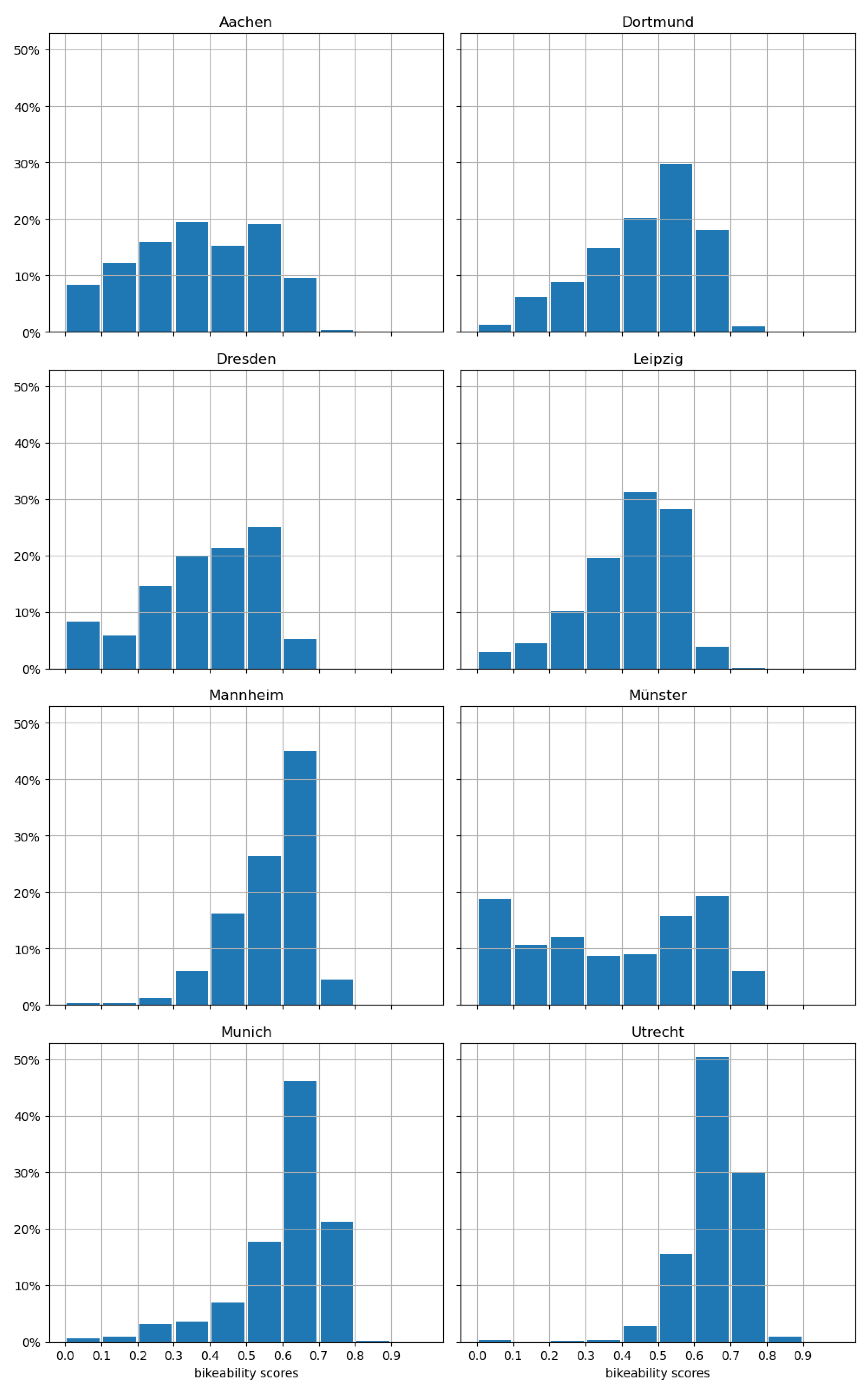
5.2. Calculated Bikeability Values

As a first step, the bikeability scores for each building in each selected city were calculated using the simulation model described in Section 3.1. The resulting scores were plotted geographically. The resulting maps are shown in Figure 2 and Figure 3. All maps that are shown in this section are also available as interactive pydeck maps [22].

For every city’s bikeability scores, mean, standard deviation and median values were calculated. As described in Section 3.1, the ten percent lowest scores of each city were discarded. This was performed in order to account for faulty connections in the underlying traffic grid. The artificially lower scores on the outermost edges of city borders are also mitigated by this. The resulting values are listed in

Table 4. Bikeability averages, median values and standard deviations for all sample cities. Only the best 90% of buildings are used. All values are original calculations.

City	n	Mean	Std	Median
Aachen	51,874	0.347	0.179	0.344
Aachen (80%)	41,494	0.402	0.152	0.396
Dortmund	154,522	0.469	0.133	0.493
Dresden	62,535	0.365	0.167	0.378
Leipzig	70,347	0.429	0.113	0.444
Mannheim	51,339	0.553	0.115	0.586
Munich	126,095	0.640	0.073	0.649
Münster	89,021	0.327	0.252	0.303
Münster (80%)	64,108	0.416	0.222	0.245
Utrecht	114,985	0.652	0.069	0.667

. This table also includes the additional analyses with smaller borders for Münster and Aachen, as described in Section 3.4. In addition to the comparison values, the table also includes the number of buildings for each city.

The results of the additional analysis of city cores is shown in

Table 5. Bikeability averages, median values and standard deviations for the cores of all sample cities. Cores are defined as a 1 km radius around the city hall. For the state capitals Munich and Dresden, a larger radius of 2 km is considered additionally. All values are original calculations.

City	n	Mean	Std	Median
Aachen	5379	0.577	0.083	0.595
Dortmund	3683	0.604	0.097	0.637
Dresden	296	0.495	0.085	0.510
Dresden (2 km)	2327	0.441	0.131	0.467
Leipzig	2365	0.515	0.055	0.522
Mannheim	3400	0.608	0.096	0.637
Munich	228	0.678	0.029	0.683
Munich (2 km)	2072	0.672	0.039	0.677
Münster	4076	0.621	0.098	0.662
Utrecht	6777	0.615	0.066	0.605

. This table also includes the wider cores for the state capitals Munich and Dresden.

In addition to averages, median values and standard deviations, histogram plots are used to evaluate the cities’ bikeability. Histogram plots for all cities are shown in Figure 4.

The bikeability scores correlate to the reference values discussed in Section 5.1 in some aspects, but differ from them significantly in others. First of all, Utrecht has the highest bikeability score out of all cities. It also has the lowest standard deviation, implying a consistent level of bikeability across the city borders. The second highest average bikeability score was calculated for Munich. Considering the comparative values discussed previously, this is surprising. Similarly, Dortmund’s score is also higher than expected. This leads to the assumption that the lower modal share for cyclists in these cities is not due to their infrastructure and topology.

Another surprising difference between bikeability scores and comparison values exists in the case Münster. The difference between the city core analysis in Table 5 and the full city analysis in Table 4 suggests that this disparity is at least partially explained by the rural–urban divide in Münster.

In order to further evaluate the assumptions made about Münster and Munich, their suitability maps are shown in Figure 5. The scores shown on these maps are normally used as the basis for the routing that is the basis of the bikeability model described in Section 3.1. In contrast to the more abstract and complex bikeability scores, bicycle suitability scores are calculated by evaluating the bicycle infrastructure for one road section in isolation. These maps confirm that Munich’s bicycle infrastructure is better than its low modal share and bicycle cities rank suggest. It also confirms the large disparity between the heavily interconnected urban parts of Münster and the less connected rural villages next to the main city.

6. Discussion and Conclusions

This study provides a comprehensive overview of a use case of bikeability calculations to compare different cities. Furthermore, bikeability metric was compared with other existing metrics of public bicycle usage. It was discovered that the assessment capability of bikeability towards bicycle friendliness is limited, as was proven by the disparity between bikeability and metrics of cyclist satisfaction like survey data and modal share, as discussed in Section 5.2. In contrast, a strong connection between bikeability and established metrics for bicycle infrastructure quality was shown.

The comparison between cities is based on statistical analyses. Further research into the socio-economic connection between bicycle infrastructure, bicycle usage and the happiness of participants of city’s traffic is necessary.

One problem connected with using bikeability to compare different cities is the differing level of urbanization between them. Different methods to mitigate this issue were evaluated. In the end, it can be concluded that the bikeability model in its current form is better suited towards analyzing the structural differences within a city than for inter-city comparisons. If further comparisons between different cities are called for, focusing on specific city quarters with structural similarities could be beneficial.

When regarding single cities, the bikeability model discussed here should be regarded as a separate tool. It has proven helpful as an objective indicator for a city’s structure and the quality of its infrastructure, but it is not a replacement for any of the established methods of evaluating the quality of bicycle traffic.

Regarding the cities themselves, the most interesting insight gained while conducting this study concerns cities that are not historically focused on bicycle traffic. These cities include Munich, Dresden, Dortmund and Leipzig. It was discovered that the low percentage of cyclists in their traffic cannot be explained by a surface-level analysis of the available infrastructure, nor by purely focusing on bikeability. Instead, research into the socio-economic reasons for low bicycle usage is necessary.

Regarding all results of this study, the limitations of the underlying bikeability model need to be made clear. As discussed in Section 3.3, the model is limited by the available input data. For the purposes of this study, a profile representing a family has been used. In future research, the development of a more representative profile could improve the quality of the results. An exemplary discussion of the results of the model’s routing algorithm as well as the impact of different weights for bicycle suitability have been conducted when developing the model. However, an extensive, empirical comparison between model data and real bicycle trips could further improve it.

References

1. Bundesministerium für Digitales und Verkehr. Fahrrad-Monitor 2023. 2023. Available online: https://bmdv.bund.de/SharedDocs/DE/Artikel/StV/Radverkehr/fahrradmonitor.html (accessed on 30 April 2025).
2. Kellershohn, J.; Maurer, F.; Jungbluth, C. Bikeability Scoring Auf Basis von Open Data—Ein Open-Source Modell. In New Players in Mobility; Springer Gabler: Wiesbaden, Germany, 2025; p. 12. [Google Scholar] [CrossRef]
3. Lowry, M.; Callister, D.; Gresham, M.; Moore, B. Assessment of Communitywide Bikeability with Bicycle Level of Service. Transp. Res. Rec. J. Transp. Res. Board 2012, 2314, 41–48. [Google Scholar] [CrossRef]
4. Winters, M.; Brauer, M.; Setton, E.; Teschke, K. Mapping Bikeability: A Spatial Tool to Support Sustainable Travel. 2013. Available online: https://journals.sagepub.com/doi/abs/10.1068/b38185 (accessed on 30 April 2025).
5. Winters, M.; Teschke, K.; Brauer, M.; Fuller, D. Bike Score®: Associations between Urban Bikeability and Cycling Behavior in 24 Cities. Int. J. Behav. Nutr. Phys. Act. 2016, 13, 18. [Google Scholar] [CrossRef] [PubMed]
6. Titze, S.; Krenn, P.; Oja, P. Developing a Bikeability Index to Score the Biking-Friendliness of Urban Environments. J. Sci. Med. Sport 2012, 15, S29–S30. [Google Scholar] [CrossRef]
7. Gehring, M.S.D.B. Bikeability—Index für Dresden—Wie fahrradfreundlich ist Dresden? Master’s Thesis, Technical University of Dresden, Dresden, Germany, 2017. [Google Scholar]
8. Schmid-Querg, J.; Keler, A.; Grigoropoulos, G. The Munich Bikeability Index: A Practical Approach for Measuring Urban Bikeability. Sustainability 2021, 13, 428. [Google Scholar] [CrossRef]
9. Hardinghaus, M. Exploring Bikeability. Ph.D. Thesis, Humboldt-Universität zu Berlin, Berlin, Germany, 2021. [Google Scholar] [CrossRef]
10. Hoedl, S.; Titze, S.; Oja, P. The Bikeability and Walkability Evaluation Table: Reliability and Application. Am. J. Prev. Med. 2010, 39, 457–459. [Google Scholar] [CrossRef] [PubMed]
11. Halldórsdóttir, K.; Rieser-Schüssler, N.; Axhausen, K.W.; Nielsen, O.A.; Prato, C.G. Efficiency of Choice Set Generation Methods for Bicycle Routes. Eur. J. Transp. Infrastruct. Res. 2014, 14, 332–348. [Google Scholar] [CrossRef]
12. Owais, M.; Alshehri, A. Pareto Optimal Path Generation Algorithm in Stochastic Transportation Networks. IEEE Access 2020, 8, 58970–58981. [Google Scholar] [CrossRef]
13. Almutairi, A.; Owais, M. Reliable Vehicle Routing Problem Using Traffic Sensors Augmented Information. Sensors 2025, 25, 2262. [Google Scholar] [CrossRef] [PubMed]
14. Fosgerau, M.; Paulsen, M.; Rasmussen, T.K. A Perturbed Utility Route Choice Model. Transp. Res. Part C Emerg. Technol. 2022, 136, 103514. [Google Scholar] [CrossRef]
15. Fosgerau, M.; Łukawska, M.; Paulsen, M.; Rasmussen, T.K. Bikeability and the Induced Demand for Cycling. Proc. Natl. Acad. Sci. USA 2023, 120, e2220515120. [Google Scholar] [CrossRef] [PubMed]
16. Broer, K. Fietsbalans II: Competitiveness Bicycle Greatly Improved—Fietsberaad. 2008. Available online: https://www.fietsberaad.nl/Kennisbank/Fietsbalans-II-competitiveness-bicycle-greatly-imp (accessed on 30 April 2025).
17. Hjalmar Christiansen, Marie Karen Anderson The Danish National Travel Survey Annual Statistical Report, 2024. DTU Center for Transport Analytics. Denmark 2024. Available online: https://www.man.dtu.dk/english/-/media/institutter/management/scientific-advice/transportvaneundersoegelsen/t-u/tu-udgivelser/tu_denmark_2024-engelsk.pdf (accessed on 30 April 2025).
18. Nobis, C.; Kuhnimhof, T. MiD Ergebnisbericht. Technical Report, Infas, DLR, IVT und Infas 360; MiD Ergebnisbericht: Bonn, Berlin, 2018. [Google Scholar]
19. Copenhagenize. Available online: https://copenhagenizeindex.eu/about/methodology (accessed on 30 April 2025).
20. Luko. Le Classement 2022 des Meilleures Villes au Monde où Faire du Vélo. Available online: https://fr.luko.eu/conseils/guide/bike-index/ (accessed on 30 April 2025).
21. ADFC. ADFC Fahrradklima-Test 2022: Städteranking. 2023. Available online: https://fahrradklima-test.adfc.de/ergebnisse (accessed on 30 April 2025).
22. Kellershohn, J. Bikeability Comparison Data for MDPI Paper, 2025. Available online: https://zenodo.org/records/15064679 (accessed on 30 March 2025).
23. Kellershohn, J.; Maurer, F. Bikeability—NOWUM Energy Git. 2024. Available online: https://github.com/NOWUM/bikeability (accessed on 30 March 2025).
24. OpenStreetMap contributors. 2017. Planet Dump. Available online: https://planet.osm.org (accessed on 30 April 2025).
25. Ferster, C.; Fischer, J.; Manaugh, K.; Nelson, T.; Winters, M. Using OpenStreetMap to Inventory Bicycle Infrastructure: A Comparison with Open Data from Cities. Int. J. Sustain. Transp. 2019, 14, 64–73. [Google Scholar] [CrossRef]
26. Boeing, G. Modeling and Analyzing Urban Networks and Amenities with OSMnx. Geogr. Anal. 2025; published online ahead of print. Available online: https://geoffboeing.com/publications/osmnx-paper/ (accessed on 30 April 2025).
27. Statistische Ämter des Bundes und der Länder. Unfallatlas. Available online: https://unfallatlas.statistikportal.de/ (accessed on 30 April 2025).
28. Städte in Bewegung. Available online: https://www.agora-verkehrswende.de/veroeffentlichungen/staedte-in-bewegung (accessed on 30 April 2025).
29. Fischer, B. Kosten Der Mobilität–Zahnlen Und Fakten Zu Den. Preisen Im Straßen- Und Schienenverkehr Sowie Deren Bedeutung Für Die Gesellschaft Und Den Klimaschutz, 2023. Available online: https://www.agora-verkehrswende.de/fileadmin/user_upload/99_Faktenblatt-Mobilitaetskosten.pdf (accessed on 30 April 2025).
30. Lumiste, M. CycloRank. 2021. Available online: https://mlumiste.com/projects/cyclorank/ (accessed on 30 April 2025).
31. Directorate-General for Research and Innovation (European Commission). EU Missions: 100 Climate Neutral and Smart Cities; Publications Office of the European Union: Luxembourg, 2024. [Google Scholar]
32. Melderegisterauswertung Stand 31.12.2024. 2025. Available online: https://www.aachen.de/aachen-entdecken/typisch-aachen/statistische-daten/melderegisterauswertung-stand-311224.pdf?cid=msj (accessed on 30 April 2025).
33. Andrä, D.; Koch, F.; Schlattmann, T. Bevölkerung in Zahlen. 2024. Available online: https://statistikportal.dortmund.de/bevoelkerung/bevoelkerunginzahlen/#bev%C3%B6lkerungsstand (accessed on 30 April 2025).
34. Dresden, L. Bevölkerungsentwicklung Laut Melderegister. 2024. Available online: https://www.dresden.de/de/leben/stadtportrait/statistik/bevoelkerung-gebiet/Bevoelkerungsbestand.php (accessed on 30 April 2025).
35. Leipzig, B. Bevölkerungsbestand. 2024. Available online: https://statistik.leipzig.de/statcity/table.aspx?cat=2&rub=1&per=q (accessed on 30 April 2025).
36. Mannheim, S. Bevölkerungsbestand 2023 in Kleinräumlicher Gliederung. 2024. Available online: https://www.mannheim.de/de/stadt-gestalten/daten-und-fakten/bevoelkerung (accessed on 30 April 2025).
37. München, S.A. Statistische Daten Zur Münchner Bevölkerung. 2024. Available online: https://stadt.muenchen.de/infos/statistik-bevoelkerung.html (accessed on 30 April 2025).
38. Bevölkerung Jahres-Statistik 2023. 2025. Available online: https://www.stadt-muenster.de/statistik-stadtforschung/zahlen-daten-fakten (accessed on 30 April 2025).
39. CBS.nl. Huishoudens; Personen Naar Geslacht, Leeftijd En Regio, 1 Januari. 2025. Available online: https://opendata.cbs.nl/statline/#/CBS/nl/dataset/71488ned/table?dl=6DF07 (accessed on 30 April 2025).
Figure 1. Plot of all comparison values from the Bicycle City Index for sample cities. Own presentation based on data from [20].
Futuretransp 05 00064 g001
Figure 2. The bikeability maps of Aachen, Dortmund, Dresden and Leipzig. Zoom levels are equalized between the maps shown in this figure and the ones in Figure 3.
Futuretransp 05 00064 g002
Figure 3. The bikeability maps of Mannheim, Munich, Münster and Utrecht. Zoom levels are equalized between the maps shown in this figure and the ones in Figure 2.
Futuretransp 05 00064 g003
Figure 4. Histogram plots for all cities’ bikeability scores.
Futuretransp 05 00064 g004
Figure 5. The suitability maps of Munich and Münster.
Futuretransp 05 00064 g005