Abstract
This work explores the classification of driving behaviors using a hybrid deep learning model that combines Convolutional Neural Networks (CNNs) with Long Short-Term Memory (LSTM) networks (ConvLSTM). Sensor data are collected from a smartphone application and undergo a preprocessing pipeline, including data normalization, labeling, and feature extraction, to enhance the model’s performance. By capturing temporal and spatial dependencies within driving patterns, the proposed ConvLSTM model effectively differentiates between normal and aggressive driving behaviors. The model is trained and evaluated against traditional stacked LSTM and Bidirectional LSTM (BiLSTM) architectures, demonstrating superior accuracy and robustness. Experimental results confirm that the preprocessing techniques improve classification performance, ensuring high reliability in driving behavior recognition. The novelty of this work lies in a simple data preprocessing methodology combined with the specific application scenario. By enhancing data quality before feeding it into the AI model, we improve classification accuracy and robustness. The proposed framework not only optimizes model performance but also demonstrates practical feasibility, making it a strong candidate for real-world deployment.
1. Introduction
Artificial intelligence (AI) has revolutionized several industries, leading to significant improvements, and the automotive sector is no exception. The classification of different driving behaviors has become a key area of focus in enhancing road safety [1,2,3,4,5].
This work aims to harness the power of neural networks to analyze and classify driving behavior. Understanding driving behavior is crucial in improving road safety and in the development of advanced driver-assistance systems (ADAS) and autonomous vehicles.
The importance of driving behavior classification is growing not only within the automotive sector but also in areas such as transport and logistics. Insights into driving behavior can lead to better fleet management, reduced fuel consumption, and improved operational efficiency. Furthermore, detailed driving behavior analysis can contribute to urban planning and public safety by providing data that support better traffic management and road design based on real-world driving patterns.
Our implementation goes beyond simply training an AI model, placing a strong emphasis on data preprocessing, which is the most critical aspect of our research. Effective preprocessing is essential for accurately classifying driving behaviors, as raw sensor data can be noisy and inconsistent.
In our approach, we use a smartphone as the primary data acquisition device, leveraging its advanced built-in sensors, including accelerometers, gyroscopes, and GPS. This method not only makes data collection accessible and scalable but also presents challenges due to the inherent variability and noise in mobile sensor readings.
To ensure high-quality input, we implement a robust preprocessing pipeline that includes data normalization to standardize values, labeling strategies to accurately categorize driving behaviors, and feature extraction to retain only the most relevant motion patterns. Through these preprocessing steps, we convert the data from the sensor domain to the maneuver domain, enabling the identification of events such as left and right turns, accelerations, and braking.
At this stage, our implemented model is only detecting aggressive and non-aggressive driving behaviors. However, in future work, we aim to extend this approach to identify specific driving maneuvers, such as turns, accelerations, and braking events. Since all the necessary preprocessing has already been completed, future models will be able to leverage this structured data to achieve more granular and precise driving behavior classification.
This preprocessing process is crucial as it transforms low-level sensor measurements into more interpretable and meaningful representations of driving behavior. As a result, our AI model receives optimized input data, significantly improving classification accuracy across different driving styles.
Thus, preprocessing is not just an auxiliary step—it forms the foundation of our work, ensuring that the AI model has access to structured, relevant, and optimized data for reliable and precise classification.
Long Short-Term Memory (LSTM) networks are well suited for driving behavior classification, as they capture intrinsic dependencies and correlations in time-series data collected during real driving sessions [1]. By leveraging LSTM networks, we aim to classify different driving behaviors, specifically distinguishing between normal and aggressive driving patterns. Our goal is to obtain the optimal LSTM model to ensure highly accurate classification.
In this paper, we propose a hybrid model that combines Convolutional Neural Networks (CNNs) with LSTM (ConvLSTM), and we compare our results with stacked LSTM and Bidirectional LSTM (BiLSTM) architectures. The proposed hybrid model outperforms traditional stacked LSTM and BiLSTM architectures in accurately classifying driving patterns, with a focus on differentiating between normal and aggressive driving behaviors.
2. Related Work
Several architectures have been proposed and evaluated for their effectiveness in driving behavior classification [1].
Previous research has demonstrated that LSTM networks excel in various sequence prediction tasks [2]. In driving behavior analysis, these models achieve high accuracy, precision, and recall when classifying different driving behaviors.
For instance, Saleh et al. [3] employed a stacked LSTM approach for driving behavior classification based on sensor data fusion, using the UAH-DriveSet dataset. Their model effectively categorized behaviors into three classes: normal, aggressive, and drowsy driving. Furthermore, combining LSTM networks with other neural models has proven to enhance classification performance. Deo and Trivedi [4] introduced an LSTM-based framework for interaction-aware motion prediction of surrounding vehicles on freeways. Their model significantly reduced prediction errors when accounting for vehicle interactions, as demonstrated on the NGSIM US-101 and I-80 datasets.
Khodairy and Abosamra [5] proposed a deep learning solution for driving behavior classification using an optimized stacked LSTM model with smartphone-embedded sensor data. Their approach supported both three-class (normal, drowsy, and aggressive) and binary classifications of driving behavior. Tested on the UAH-DriveSet dataset, their model achieved F1 scores of 99.49% and 99.34%, respectively, outperforming prior state-of-the-art techniques.
Beyond driving behavior analysis, LSTM networks have demonstrated high efficiency across various domains [6,7,8,9,10,11,12,13]. In financial forecasting, LSTM and ConvLSTM outperformed ARIMA and Support Vector Regression (SVR) in predicting orange juice futures, effectively capturing temporal dependencies and reducing prediction errors [9]. In building occupancy prediction, a hybrid Graph Neural Network (GNN) and LSTM model outperformed RNNs and GRUs, achieving better alignment with reference profiles [10]. LSTM also excelled in electromyographic signal classification, achieving 98.46% accuracy with superior processing speed compared to GRU and bidirectional networks, further optimized using the Grey Wolf Algorithm [11]. In industrial applications, an LSTM-based model minimized oscillations in overhead cranes, enhancing safety and control [12]. Similarly, in fuel consumption prediction, integrating “jerk” as a variable improved accuracy, particularly in high-speed scenarios, with LSTM showing the most significant gains under expressway conditions [13].
These studies underscore LSTM’s adaptability in temporal modeling and process optimization.
3. Proposed Methodology
3.1. Problem Statement
The rapid advancement of Intelligent Transport Systems (ITSs) has paved the way for seamless wireless communication between vehicles (V2V) and between vehicles and infrastructure (V2I). This capability facilitates the exchange of critical information, which plays a crucial role in enhancing traffic management, improving road safety, and increasing overall transportation efficiency. As ITSs continue to evolve, accurately classifying driver behavior becomes essential for developing adaptive, intelligent, and responsive transportation solutions.
This paper addresses the challenge of classifying driver behavior exclusively using artificial intelligence (AI) techniques, leveraging data collected through a mobile application. Unlike traditional approaches that rely on external hardware or sensors, this method aims to develop a purely software-based solution, making it more accessible and cost-effective.
The core focus of this research is on training a neural network model for analyzing and classifying driving patterns. Given the sequential nature of driving data, LSTM networks are particularly well suited for this task. LSTMs excel at learning temporal dependencies and recognizing sequential patterns, making them an ideal choice for capturing the complexities of driver behavior.
The ultimate goal of this study is to develop a highly resilient and accurate LSTM-based model capable of predicting driver behavior within an ITS framework. By achieving this, the research has the potential to contribute significantly to traffic management strategies, reduce accident rates, and enhance overall transportation safety and efficiency.
To implement and validate the proposed approach, the research was conducted using the Python version 3.11.4 programming language. The entire workflow, including data preprocessing, model development, and evaluation, was carried out using the Visual Studio Code IDE version 1.99.1, ensuring a robust and scalable development environment.
3.2. Long Short-Term Memory Neural Networks
The LSTM network is an improved version of the RNN designed by Hochreiter and Schmidhuber [6]. LSTM is well suited for sequence prediction tasks and excels at capturing long-term dependencies.
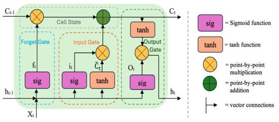
A traditional RNN has a single hidden state that is transmitted over time, which can make it difficult for the network to learn long-term dependencies. LSTM networks solve this problem by introducing a memory cell, which is a container that can store information for an extended period of time [7]. Figure 1 illustrates an LSTM cell.
Figure 1.
Diagram of LSTM cell [14].
An LSTM network includes a series of memory cells and blocks responsible for storing and processing information over time. Every LSTM cell holds three gates: the Input Gate, the Forget Gate, and the Output Gate.
The Forget Gate (ft) determines what portion of the previous cell state should be discarded (Equation (1)).
where Wf and bf are the weights and biases for the forget gate; ht−1 is the hidden state from the previous time step; xt is the input at the current time step; and sig is the sigmoid activation function, ensuring values range between 0 and 1.
ft = (Wf [ht−1, xt] + bf)
The Input Gate (it) controls how much new information should be added to the cell state (Equation (2)).
where it controls how much new information is added to the memory cell.
it = sig(Wi [ht−1, xt] + bi)
Cell State Update (ĉt) proposes an update to the memory cell (Equations (3) and (4)).
where Ct−1 is the previous cell state and ⊙ represents element-wise multiplication. The cell state is updated by forgetting part of the previous state and adding new information.
ĉt = tanh (WC [ht−1, xt] + bC)
Ct = ft⊙Ct−1 + it⊙ĉt
The Output Gate (ot) decides what part of the cell state should be output at the current time step (Equations (5) and (6)).
where the output gate ot determines how much of the updated cell state should be passed to the next layer. The hidden state ht is computed by applying the tanh activation function to the cell state and filtering it using the output gate.
ot = sig(Wo [ht−1, xt] + bo)
ht = ot ⊙ tanh(Ct)
3.3. Long Short-Term Memory Networks Combined with Convolutional Neural Networks
CNNs, particularly Conv1D, are computationally less demanding and therefore faster to train and execute compared to traditional LSTM networks. This architecture excels at extracting relevant patterns from subsequences, significantly enhancing the results’ quality.
The most notable benefit of Conv1D is its flexibility in being combined with other architectures, such as LSTM networks, to further improve performance and scalability. Section 3.9 details our model.
This hybrid design leverages Conv1D for feature extraction while using fully connected layers for classification.
3.4. Data Collecting and Processing
The dataset used in this study was collected through a dedicated mobile application specifically developed for data acquisition. This application utilizes smartphone sensors, including the accelerometer, gyroscope, and GPS, to capture driving-related data in real-world conditions. By designing our own data collection framework, we ensured control over the data quality, sampling rates, which enhances the reliability and applicability of the dataset for AI-based driving classification models.
The smartphones used for data collection were consistently positioned in the same horizontal orientation, with the front side facing upward and the Y-axis of the accelerometer aligned with the front of the vehicle. Maintaining a standardized placement ensured consistency in data acquisition, reducing variability that could affect model performance.
The decision to not use vehicle-integrated sensors was driven by our objective: developing a generalized, portable solution that can be deployed on any mobile device. This approach ensures compatibility across different vehicle models, making the system more practical and accessible for a broader range of users.
Additionally, in European vehicles, only Event Data Recorder (EDR) data are mandated, meaning that built-in vehicle sensors do not consistently provide access to the full spectrum of sensor readings required for our solution. Many manufacturers restrict direct access to proprietary sensor data, further limiting the feasibility of relying on vehicle-integrated systems.
By leveraging smartphone-based sensors, we achieve several key advantages:
- Flexibility—Users can deploy the system in any vehicle without hardware modifications;
- Accessibility—No dependence on manufacturer-specific data access policies;
- Interoperability—Ensures compatibility across different makes and models, increasing adoption potential.
This approach makes our solution not only more adaptable but also scalable, as it does not rely on proprietary vehicle hardware, ensuring long-term usability regardless of automotive industry changes.
The data processing involved the identification and categorization of various driving maneuvers, including the following:
- Sudden accelerations and decelerations;
- Turns and lane changes;
- Abrupt stops and starts.
These maneuvers were detected using accelerometer and gyroscope sensors from smartphones along the X, Y, and Z axes. In general, accelerometers measure linear acceleration, while gyroscopes capture angular velocity.
After data collection, a preprocessing step was applied to separate positive and negative values. This approach ensured that the model remained unaffected by potentially negative numbers, maximizing its predictive accuracy. As a result, two separate columns were created: one containing only positive values and another containing only negative values, both derived from the respective sensor readings. In the first column, the negative values are set to 0, and in the second column, the negative values are replaced with their absolute values, while the positive values are set to 0.
Next, these two columns were structured into a 2D array with a total of twelve elements—six positive and six corresponding negative values extracted from the processed sensor data. Table 1 presents examples of the collected data and Table 2 shows the values of the 12 columns after processing sensor data.

Table 1.
Examples of collected data.
Table 2.
Examples containing 12 columns with the processed sensor data.
3.5. Data Classification
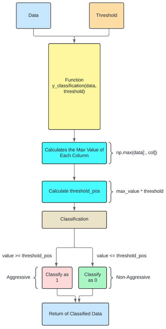
The classification workflow is visually represented in Figure 2, illustrating the step-by-step transformation of raw data into categorized outputs.
Figure 2.
Diagram of data classification process.
The classification process begins by inputting two key parameters into the function y_classification(data, threshold): data and threshold. The primary objective of this function is to return a Boolean classification for each data point, distinguishing between aggressive and non-aggressive behavior. Specifically, the function assigns a value of 1 to indicate aggressive behavior and 0 for non-aggressive behavior. To store these classifications, an output_vector is initialized, which will ultimately hold the results of the classification process.
To achieve this, the function iterates through all 12 columns of the dataset, computing the maximum value for each column. This computation is performed using the NumPy function np.max(data[:, col]), which extracts the highest value in each respective column. Once these maximum values are obtained, a threshold-based comparison value, threshold_pos, is calculated by multiplying each maximum value by the specified threshold parameter (threshold_pos = max_value * threshold).
The classification of data points is then executed according to the following logic:
- If a given data value is greater than or equal to threshold_pos, it is classified as 1 (aggressive behavior).
- If a given data value is less than threshold_pos, it is classified as 0 (non-aggressive behavior).
After processing all values in the dataset, the initialized output_vector is populated with the classification results. Finally, this vector, containing the classified data, is returned as the function’s output.
Using the data obtained from the sensors, it was possible to determine the threshold values for classifying aggressiveness. This parameter can be continuously adjusted based on new tests.
This approach ensures a systematic classification process based on the specified threshold, allowing for the identification of aggressive behavior patterns within the dataset.
3.6. Data Normalization
To enhance the performance of the model, the dataset underwent a normalization process. Normalization involves scaling the values of each variable to a common range, ensuring consistency across different sensor readings. In this case, the data were normalized within the interval [0, Max Value of Each Sensor Set], which helps improve the stability and efficiency of the model during training and evaluation.
The normalization process begins with the application of the max_of_vectors function, which determines the maximum value across selected sensor readings. This function can operate in two variations depending on the type of sensor being processed.
For accelerometer data, the function takes the following input parameters (see Table 2):
- AccelRight (positiveX), AccelLeft (negativeX), AccelForward (positiveY), AccelBackward (negativeY), AccelUp (positiveZ), and AccelDown (negativeZ).
For gyroscope data, the input parameters include the following:
- GyrPitchUp (positiveX), GyrPitchDown (negativeX), GyrRollRight (positiveY), GyrRollLeft (negativeY), GyrYawRight (positiveZ), and GyrYawLeft (negativeZ).
Normalization is achieved by dividing each data point by the computed maximum value for the corresponding column. This transforms the raw values into a scaled range, effectively rescaling all sensor readings proportionally. As a result, every value in the dataset is normalized between 0 and 1, based on the maximum value of each sensor’s readings.
This normalization step is essential for several reasons. First, it removes scale bias, ensuring that features with larger magnitudes do not dominate the model. Second, it allows for the standardization of data from different sensors, enabling smoother integration of multi-sensor inputs. Third, normalization improves machine learning model performance by stabilizing training, accelerating convergence, and preventing numerical instability. By rescaling the data to a uniform range, the model can learn more effectively, focusing on the relative differences between values rather than their absolute magnitudes.
By applying this normalization technique, the dataset maintains consistency, reducing discrepancies between sensor readings and enhancing the model’s ability to detect patterns accurately.
3.7. Split Data into Training and Test Sets
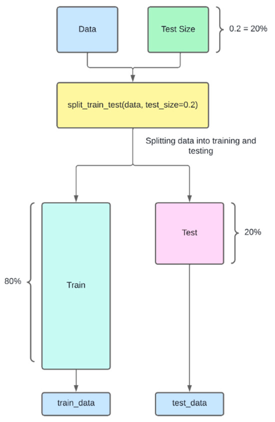
The model is tested on part of the data divided for training and testing. This was carried out in a ratio as follows:
- 80%: training data;
- 20%: testing data.
The process of dividing the data into training and testing sets used the function split_train_test(data, test_size = 0.2). The input parameters to the function are the data and the size of the test data sequence. The size parameter directly impacts the size of the training sequence.
Specifically, test_size = 0.2 means 20% of the data will be used for testing the model, while the remaining 80% stays in the train sequence. This is an equal and fair split to both so that training can be effectively carried out based on it and performance evaluation can also be reliable. The split was performed randomly. The shuffle was set to true in the model definition.
Figure 3 outlines the data separation process.
Figure 3.
Diagram of data separation process.
3.8. Data Representation
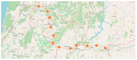
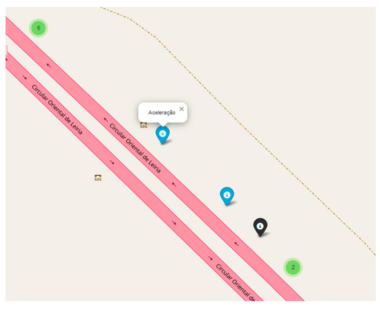
For a better analysis of the recorder maneuvers, we used the Folium Library to create an interactive map. A marker cluster was added to the map to visually group nearby events.
Markers were then added for each recorder position, differentiated by colors to represent different types of maneuvers. Figure 4 presents a plot of the dataset maneuvers; the numbers indicate the total number of aggressive maneuvers captured in each zone. Figure 5 provides a zoomed-in plot of the dataset maneuvers.
Figure 4.
Plot of dataset maneuvers.
Figure 5.
Plot of zoomed dataset maneuvers.
3.9. Model Construction
For comparison purposes, we include the summary of the models ConvLSTM, BiLSTM, and StackedLSTM, and we provide a detailed description of the ConvLSTM model for the sake of reproducibility.
The selection of stacked LSTM and BiLSTM as benchmarks was based on their relevance to time-series modeling and their ability to capture temporal dependencies in sequential data. Stacked LSTM and BiLSTM are widely used in driving behavior analysis and time-series modeling, making them strong and well-understood baselines for evaluating ConvLSTM [3,4,5,6,7].
Since driving behavior is inherently sequential, we prioritized models designed to capture temporal dependencies. StackedLSTM allows for deeper feature extraction, while BiLSTM captures both forward and backward dependencies, providing a fair comparison to ConvLSTM.
The selection of hyperparameters was based on preliminary observations and empirical experimentation. We conducted a series of initial tests to identify the most suitable values for the hyperparameters, observing their impact on model performance. This process allowed us to make an informed choice, considering the model’s complexity and the nature of the data used. While we did not perform exhaustive formal optimization, the choices were based on the best practices and insights gained during the preliminary experimentation phase.
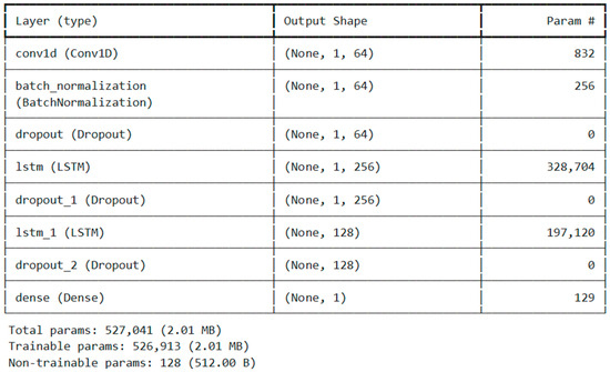
The model ConvLSTM adopted in the present study is a hybrid architecture that presents both CNNs with one dimension (Conv1D) and LSTM networks, which is designed for the classifier of driving behaviors based on sensor data. Figure 6 presents the model summary of our model.
Figure 6.
Model summary of ConvLSTM.
This ConvLSTM model combines a Conv1D layer with LSTM layers to extract both spatial and temporal patterns from sequential data.
It starts with a Conv1D layer that captures local spatial features, outputting a (1, 64) shape feature map. A batch normalization layer follows, stabilizing activations, and a dropout layer helps prevent overfitting.
Next, the data pass through the first LSTM layer, which learns long-term dependencies, expanding the output to (1, 256). Another dropout layer helps regularize the network. A second LSTM layer further refines the sequence representation, reducing the dimensionality to (128), followed by another dropout layer.
Finally, a dense layer with 1 output neuron produces the final prediction. The model has 527,041 total parameters, with 526,913 trainable and a small number of non-trainable parameters (128).
This architecture is ideal for time-series forecasting, anomaly detection, or sequence classification, as it efficiently extracts both local spatial patterns and long-term dependencies. This hybrid design leverages Conv1D for feature extraction while using fully connected layers for classification.
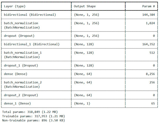
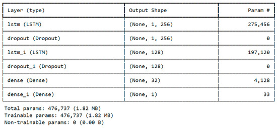
Figure 7 illustrates the architecture of the BiLSTM model and Figure 8 illustrates the StackedLSTM model.
Figure 7.
Model summary of BiLSTM.
Figure 8.
Model summary of StackedLSTM.
In the next section, we describe the hyperparameters used by the ConvLSTM model.
3.9.1. Model Architecture
- Conv1D Layer:
- Filters: 64;
- Kernel Size: 1;
- Activation: ReLU;
- Input Shape: (number of time steps, number of features).
Conv1D is the convolutional layer that helps to extract local features from time-series input data, using 64 such filters of size 1 to capture fine-grained patterns in these data.
- 2.
- Batch Normalization:
This layer helps to normalize the output of the Conv1D layer in order to increase training stability and speed.
- 3.
- Dropout Layer:
- Dropout Rate: 0.5.
Dropout aims to prevent overfitting, as it randomly sets half of the Conv1D layer output units to zero during training.
- 4.
- Primary LSTM Layer:
- Units: 256;
- Return Sequences: True.
The first LSTM layer captures the temporal dependencies within the data and returns sequences for processing by the next LSTM layer.
- 5.
- Dropout Layer:
- Dropout Rate: 0.2.
For the prevention of overfitting, dropout is applied to the output of the first LSTM layer.
- 6.
- LSTM Layer (Middle):
- Units: 128.
The second layer of the LSTM network further deals with the temporal dependencies existing in data, reducing the output to a fixed-size vector.
- 7.
- Dropout Layer:
- Dropout Rate: 0.2.
To prevent overfitting, the output of the second LSTM layer is passed to a Dropout layer.
- 8.
- Dense Layer:
- Units: 1;
- Activation: Sigmoid.
The dense layer using 1 unit and the activation function sigmoid gives the final classification scores for each class.
3.9.2. Model Compilation
The model was built using the following parameters:
- Optimizer: Adam;
- Loss function: Binary Cross-Entropy;
- Metrics: Accuracy.
The selection of hyperparameters was based on preliminary observations and empirical experimentation. We conducted a series of initial tests to identify the most suitable values for the hyperparameters, observing their impact on model performance. This process allowed us to make an informed choice, considering the model’s complexity and the nature of the data used. While we did not perform exhaustive formal optimization, the choices were based on best practices and insights gained during the preliminary experimentation phase.
The Adam optimizer employs high-level adaptive learning rates and demonstrates efficiency, which may alleviate the typical problems of training deep neural networks [8]. The binary cross-entropy loss is selected as the criterion based on which the structure is optimized, and the model is evaluated through validation using accuracy. This makes the hybrid Conv1D-LSTM model able to extract the strengths of these convolutional and recurrent layers to derive spatial and temporal features from sensor data, making it good at performance in driving behavior classification.
4. Experiments
In our experiments, we focused on comparing several advanced deep learning models, including stacked LSTM, ConvLSTM, and BiLSTM, to evaluate their effectiveness in capturing complex temporal and spatial dependencies. The selection of these models is motivated by their proven ability to process sequential data, making them well suited for tasks involving time-series analysis and spatiotemporal relationships.
Stacked LSTM leverages multiple layers of LSTM units to extract hierarchical temporal features, enhancing its capacity to learn long-term dependencies. ConvLSTM integrates convolutional operations within the LSTM framework, making it particularly effective in scenarios where spatial features play a crucial role alongside temporal patterns. BiLSTM, on the other hand, processes input sequences in both forward and backward directions, capturing past and future contextual information simultaneously.
By comparing these models, we aim to determine their respective strengths and limitations in handling driving behavior classification, ultimately identifying the most effective approach for this application.
All the experiments were performed on an AI server powered by an NVIDIA A100 GPU; however, this work does not consider server processing performance a relevant metric.
4.1. DataSet
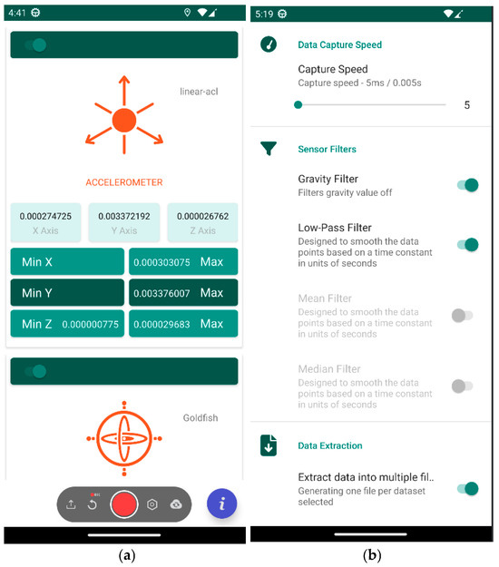
A mobile application was developed to collect data from the accelerometer and gyroscope across various pre-defined routes, ensuring the inclusion of as many maneuvers as possible. Figure 9a shows the main capture interface and Figure 9b shows the configuration parameter interface.
Figure 9.
Smartphone application for data collection (a) and configuration parameters (b).
The data used in our study are derived from real driving scenarios, collected using two vehicles. Since the data were obtained in a controlled environment, factors such as the time of day and the type of road are not relevant for detecting aggressive driving behavior. The primary focus of our analysis is on the driving patterns themselves, which remain consistent regardless of these external factors.
The data obtained from the mobile application can be exported to JSON and CSV formats.
Below, we describe the CSV structure of our dataset:
- Label: The name identifier for the dataset.
- CreatedAt: The exact time and date when the dataset was created.
- CaptureSpeed: The data capture frequency in milliseconds.
- GravityFilter: An option to, if on, remove the gravitational effect from accelerometer values.
- AverageFilter: Smoothes sensor values.
- ElapseTimeInSeconds: The duration in seconds when the data have been captured.
- Device Information:
- AndroidID: A Unique Identifier for the device;
- Name: User-defined device name;
- Manufacturer: Device brand name;
- Brand: The brand of the device;
- Model: The device model;
- Accelerometer: This includes maximum range, sensor name, minimum delay, and readings on X, Y, and Z axes;
- Gyroscope: This includes maximum range, sensor name, minimum delay, and readings on X, Y, and Z axes;
- Location Data: The latitude, longitude, and speed in km/h.
- Timestamp: The date and time for every entry of data.
Data processing is described in Section 3.4.
4.2. Training
The selection of accuracy as the primary metric for our LSTM model is based on its relevance to the driving behavior classification problem and the inherent strengths of LSTM networks.
First, accuracy is the most intuitive and interpretable metric for correctly identifying driving behaviors. It measures the percentage of correct predictions relative to the total number of predictions made by the model, providing a clear and transparent assessment of model performance.
Additionally, accuracy is particularly suitable for our driving behavior dataset as it offers a straightforward summary of the model’s performance during testing. While other metrics may be influenced by factors such as class imbalance or outliers, accuracy provides an unbiased measure of the model’s ability to identify both common and rare driving behaviors.
To enhance the performance of the ConvLSTM model and mitigate overfitting, we incorporated callbacks during training. The ModelCheckpoint callback ensured that only the best-performing model was retained by saving the model whenever the validation loss (val_loss) improved from the previous epoch. As a result, only the model with the lowest validation loss was used for final evaluation and deployment.
Additionally, we implemented an early stopping callback, which paused the training process if the validation loss failed to improve for several consecutive epochs. This approach prevented overfitting while optimizing training efficiency.
The model was trained using the fit method with the training set (train and y_train) and validated with the validation set (test and y_test). Training was conducted for up to 30 epochs with a batch size of 256, though the early stopping callback could terminate training earlier if no further improvement was observed.
4.3. Performance Evaluation
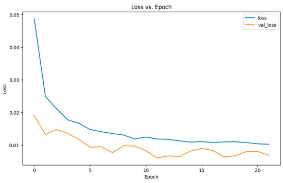
As shown in Figure 10, the training and validation losses converged within 30 epochs. The plot clearly illustrates that both losses decrease sharply during the initial epochs before stabilizing. This indicates that most models effectively learn from the training data and generalize well to their respective validation sets.
Figure 10.
Loss and Val_Loss throughout epochs.
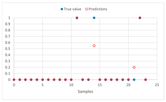
The plot in Figure 11 illustrates a portion of the test data, comparing the model’s predictions with the true values. The blue dots represent the actual values from the dataset, while the red circles correspond to the model’s predictions. This visualization helps assess the accuracy of the model by showing the degree of alignment between predicted and true values. According to the classification threshold, where predictions above 0.5 are labeled as ‘aggressive’ and those below 0.5 as ‘non-aggressive’, all samples in this plot were correctly classified. Even though some predictions do not exactly match the true values, they fall on the correct side of the threshold, demonstrating the model’s effectiveness in making accurate categorical distinctions.
Figure 11.
Model performance graph.
This analysis highlights the model’s ability to generalize well and correctly classify samples, even when minor deviations exist between predicted and actual values.
4.4. Result Comparison
The evaluation of the implemented models was conducted using a combination of metrics and visualizations to ensure a comprehensive assessment. Key evaluation aspects include accuracy across training epochs, along with other essential performance metrics such as precision, recall, F1 score, Hamming loss, and Jaccard score.
Table 3 presents a comparative analysis of these metrics across the developed models. As observed, all models demonstrate high accuracy, with the proposed ConvLSTM model achieving an accuracy of 99.75%. This indicates that, in most cases, the models successfully classified driving behavior.
Table 3.
Metric comparison between models.
Additionally, the precision and recall scores are notably high, particularly for the ConvLSTM and stacked LSTM models, highlighting their effectiveness in detecting relevant driving behaviors while minimizing false positives and false negatives. The F1 score, which represents the harmonic mean of precision and recall, further supports the balanced performance of these models, with the ConvLSTM model leading at 99.75%.
The low Hamming loss values reflect the minimal fraction of incorrectly predicted labels, with the proposed ConvLSTM achieving an impressively low Hamming loss of just 0.25%. Additionally, high Jaccard scores indicate a strong overlap between predicted and actual driving behaviors, with the ConvLSTM model again leading at 99.50%.
Overall, the proposed ConvLSTM model consistently outperforms the other architectures across multiple metrics, demonstrating its superior ability to capture and predict driving behaviors with high accuracy and reliability. These findings highlight its potential for real-world applications where precise driving behavior classification is critical.
5. Conclusions
In this work, we propose a ConvLSTM model for driving classification problems which we compare with other two LSTM-based models: the stacked LSTM and Bidirectional LSTM. This study is carried out to find the efficiency of each architecture in capturing temporal dynamics from driving data and their robustness across different driving conditions. ConvLSTM model was able to capture features in both the spatial and time domains, outperforming others in scenarios that required detailed analysis in the space-time dimension.
Our experimental results confirmed that the preprocessing techniques, including data normalization, labeling, and feature extraction, significantly enhanced classification performance, ensuring high reliability in distinguishing between normal and aggressive driving behaviors.
Although the ConvLSTM model was promising, there are a number of topics that clearly open up avenues for further investigation. Future research shall be focused on the optimization of these models for real-time applications, where scalability remains challenging. Expanding training datasets to hold more varied driving environments will increase model robustness. Further development of methods for interpretability is also required to make AI systems able to provide clear and human-understandable explanations for their decisions. Additionally, future work should aim not only to determine whether a maneuver was aggressive but also to classify the specific type of maneuver performed, further enhancing the system’s applicability in real-world driving scenarios.
Author Contributions
All authors contributed equally to this work. Conceptualization, S.M., P.L. and A.B.; investigation, A.P., J.C., S.M., P.L. and A.B.; methodology, S.M., P.L. and A.B.; resources, A.P., J.C. and P.L.; supervision, S.M., P.L. and A.B.; validation, A.P., J.C., S.M., P.L. and A.B.; writing—original draft, A.P., J.C., S.M., P.L. and A.B.; writing—review and editing, A.P., J.C., S.M., P.L., A.B., R.M. and I.H. All authors have read and agreed to the published version of the manuscript.
Funding
This work was supported by national funds through the Portuguese Foundation for Science and Technology (FCT) under the project UIDB/04524/2020.
Institutional Review Board Statement
Not applicable.
Informed Consent Statement
Not applicable.
Data Availability Statement
The original contributions presented in this study are included in the article. Further inquiries can be directed to the corresponding author.
Conflicts of Interest
The authors declare no conflicts of interest related to this work.
References
- Bouhsissin, S.; Sael, N.; Benabbou, F. Driver Behavior Classification: A Systematic Literature Review. IEEE Access 2023, 11, 14128–14153. [Google Scholar] [CrossRef]
- Darsono, A.M.; Mat Yazi, N.H.; Ja’Afar, A.S.; Othman, M.A.; Ahmad, M.I. Utilizing LSTM Networks for the Prediction of Driver Behavior. Prz. Elektrotechniczny 2024, 100, 182–185. [Google Scholar] [CrossRef]
- Saleh, K.; Hossny, M.; Nahavandi, S. Driving behavior classification based on sensor data fusion using LSTM recurrent neural networks. In Proceedings of the 2017 IEEE 20th International Conference on Intelligent Transportation Systems (ITSC), Yokohama, Japan, 16–19 October 2017; pp. 1–6. [Google Scholar] [CrossRef]
- Deo, N.; Trivedi, M.M. Multi-Modal Trajectory Prediction of Surrounding Vehicles with Maneuver based LSTMs. In Proceedings of the 2018 IEEE Intelligent Vehicles Symposium (IV), Changshu, China, 26–30 June 2018; pp. 1179–1184. [Google Scholar] [CrossRef]
- Khodairy, M.A.; Abosamra, G. Driving Behavior Classification Based on Oversampled Signals of Smartphone Embedded Sensors Using an Optimized Stacked-LSTM Neural Networks. IEEE Access 2021, 9, 4957–4972. [Google Scholar] [CrossRef]
- Hochreiter, S.; Schmidhuber, J. Long Short-term Memory. Neural Comput. 1997, 9, 1735–1780. [Google Scholar] [CrossRef] [PubMed]
- Al-Selwi, S.M.; Hassan, M.F.; Abdulkadir, S.J.; Muneer, A.; Sumiea, E.H.; Alqushaibi, A.; Ragab, M.G. RNN-LSTM: From applications to modeling techniques and beyond—Systematic review. J. King Saud Univ. Comput. Inf. Sci. 2024, 36, 102068. [Google Scholar] [CrossRef]
- Kingma, D.P.; Ba, J. Adam: A Method for Stochastic Optimization. arXiv 2014, arXiv:1412.698. [Google Scholar] [CrossRef]
- Ampountolas, A. Forecasting Orange Juice Futures: LSTM, ConvLSTM, and Traditional Models Across Trading Horizons. J. Risk Financ. Manag. 2024, 17, 475. [Google Scholar] [CrossRef]
- Xie, Y.; Stravoravdis, S. Generating Occupancy Profiles for Building Simulations Using a Hybrid GNN and LSTM Framework. Energies 2023, 16, 4638. [Google Scholar] [CrossRef]
- Aviles, M.; Alvarez-Alvarado, J.M.; Robles-Ocampo, J.-B.; Sevilla-Camacho, P.Y.; Rodríguez-Reséndiz, J. Optimizing RNNs for EMG Signal Classification: A Novel Strategy Using Grey Wolf Optimization. Bioengineering 2024, 11, 77. [Google Scholar] [CrossRef] [PubMed]
- Cui, X.; Chipusu, K.; Ashraf, M.A.; Riaz, M.; Xiahou, J.; Huang, J. Symmetry-Enhanced LSTM-Based Recurrent Neural Network for Oscillation Minimization of Overhead Crane Systems during Material Transportation. Symmetry 2024, 16, 920. [Google Scholar] [CrossRef]
- Zhang, L.; Ya, J.; Xu, Z.; Easa, S.; Peng, K.; Xing, Y.; Yang, R. Novel Neural-Network-Based Fuel Consumption Prediction Models Considering Vehicular Jerk. Electronics 2023, 12, 3638. [Google Scholar] [CrossRef]
- Smagulova, K.; James, A.P. Overview of Long Short-Term Memory Neural Networks. In Deep Learning Classifiers with Memristive Networks. Modeling and Optimization in Science and Technologies; James, A., Ed.; Springer: Cham, Switzerland, 2020; Volume 14, pp. 139–153. [Google Scholar] [CrossRef]
Disclaimer/Publisher’s Note: The statements, opinions and data contained in all publications are solely those of the individual author(s) and contributor(s) and not of MDPI and/or the editor(s). MDPI and/or the editor(s) disclaim responsibility for any injury to people or property resulting from any ideas, methods, instructions or products referred to in the content. |
© 2025 by the authors. Licensee MDPI, Basel, Switzerland. This article is an open access article distributed under the terms and conditions of the Creative Commons Attribution (CC BY) license (https://creativecommons.org/licenses/by/4.0/).