1. Introduction
A safe, efficient and environmentally friendly air transportation system should offer infrastructure and procedures to ensure that limited resources, such as airspace and airport capacity, are used efficiently. Therefore, the Air Traffic Flow Management (ATFM) has been established for a proper demand-capacity balancing at both local and global levels [
1,
2]. The focus of successful flow management lies therefore in efficient utilization of the current airport and airspace capacity, allowing the air traffic demand to be satisfied in a controlled manner [
3]. However, scheduled flight plans and operational variances on the day of operations frequently increase the demand on short notice.
Several factors could cause differences between planned and actual operations. For example, system inherent uncertainties (e.g., reactionary delays), external factor disturbances (e.g., weather conditions at the airport) or effects of changing wind conditions during the flight, flight interruptions (e.g., cancellations), the use of alternate airports, or airspace activities (e.g., reduced sector capacity or temporary activated restricted areas).
To counteract these short-term inconsistencies, different, mostly continent-specific concepts for dealing with poorly predictable disruptions have been developed. For example, the Long-Range Air Traffic Management (LR-ATFM) idea was evaluated in 2018 in the Asia-Pacific (APAC) area to improve demand capacity management by extending the present time horizon to complement regional ATFM implementations. As a result, substantial traffic flows could be successfully controlled with long-range situational awareness and more transparent traffic management facilitated by an early provision of target times over a waypoint and projected landing times. The LR-ATFM has been thoroughly tested and flight testing has revealed significant performance improvements.
In this framework, we would like to identify the most efficient methods to regulate the utilization of aircraft in an airport approach sector by controlling long-haul flows and the optimum time horizon for LR-ATFM control mechanisms. Thereby, short- and medium-haul arrivals are considered as uncontrolled boundary conditions. We investigate whether long-distance flights can be regulated as a flow, or whether individual, flight-specific performance limits and weather require consideration at the basis of a single flight. We also investigate the time frame within which a flight can be predicted. To answer the research question, we control 26 long-haul flights approaching Changi airport WSSS individually to investigate the possibility of transferring the findings to a flow-based approach. We control the single aircraft speed and the lateral route with corresponding fuel burn and arrival time and limit the maximal aircraft utilization in the approach sector by considering a minimum total fuel burn.
2. State of the Art
2.1. Air Traffic Flow Management in Asia
Strategic arrival management at high-frequency airports is the key to reducing both arrival delay time and traffic congestion. This so-called accommodation of the arrival traffic flow is already laid down by current and future ATFM-related research initiatives. However, in different parts of the world, different general principles and operational notions are applied. For example, in Europe, a centralized network manager from EUROCONTROL is responsible for implementing ATFM activities [
4]. Thereby, the central element for controlling air traffic in Europe is the allocation of departure slots and the definition of Calculated Take Off Time (CTOT) [
4,
5]. Traffic management initiatives such as ground delay programs or rerouting are used predominantly in the USA [
6,
7]. In Asia, on the other hand, regional associations of Air Traffic Flow Management Unit (ATFMU)s are established to improve the coordination of traffic flows, such as the Multi-Nodal ATFM concept in the APAC region [
8] or the Northeast Asia Regional ATFM Harmonization Group (NARAHG) [
9]. To handle the traffic volumes more efficiently, new concepts for traffic control are necessary, such as Trajectory-Based Operations (TBO)s [
10], dynamic demand capacity balancing [
11], or improved data transfer between responsible authorities [
12].
The International Civil Aviation Organization (ICAO) recommends two components of aircraft arrival management: flow-based controls and time-based tactical controls [
13]. In flow-based control methods of ATFM, the take-off time of arrivals at their departure airports is calculated to balance traffic needs and airspace or airport capacity per time window. Time-based controls are covered by an Arrival Manager (AMAN) who manages synchronized arrival traffic by controlling time-spacing among incoming aircraft [
14]. In this context, the extended AMAN concept attempts to move the responsibility for aircraft sequencing from the terminal area to the adjacent en-route airspace.
Specifically, within a radius of 500 NM around the airport, 20% of the delay could be shifted from the Terminal Manoeuvring Area (TMA) to the aircraft cruising phase by speed modifications [
15]. The beneficial effect of moving delays from the airport to the cruise phase using speed modifications has already been established in [
16]. Additionally, the potential of an arrival time prediction at established waypoints along the flight path on an increased capacity utilization has been qualified by Dhief et al. [
17], although without any flight performance consideration and without taking meteorological data into account.
Schultz et al. [
18] already executed an application analysis of the LR-ATFM concept in WSSS by optimizing the arrival time of 26 long-haul flights at WSSS several hours before arrival by adjusting the aircraft ground speed. However, again, no flight performance and weather constraints are taken into account. Instead, the actual arrival times have been provided to the optimizer as a probability density function. From this it follows that the potential of ground speed adjustments might be limited, taking wind speed and wind direction as well as the maximum Mach number and the stall speed into account. Furthermore, (fuel) efficiency issues are not considered.
This study provides insights into the efficiency of LR-ATFM, respecting the impact of weather and flight performance for each individual long-haul flight. Additionally, we consider possible alternative routes extracted from historical ADSB-B data and choose the most fuel-efficient scenario amongst all solutions. Therefore, we use discrete arrival times of 26 long-haul flights to the WSSS airport within one peak hour. Complementing [
18], we use the same set of flights and the same arrival times of flights in the WSSS approach sector. Similarly, we adopt the maximum capacity of 20 simulated flight movements in the approach sector.
2.2. Sector Capacity Optimization
Since the problem of minimizing the used capacity in the network is the same as in work shift scheduling problems (SSP), we implement the model and method of this type of scheduling problem to model our situation. As can be seen in
Figure 1, there is a required number of employees and a predetermined set of available workers in the shift scheduling problem, also known as the shift levelling problem. The objective of this problem is to assign workers in such a way that the required number of workers is met. The other objective of the problem is to assign workers in such a way that there is as little work overcapacity as possible. This study employs the second notion of this kind of problem and tries to have less violation from the defined capacity. Flights can be regarded as workers, and the sector’s capacity as the needed number of workers, with the caveat that our attitude should shift from the minimum required to the maximum permissible workforce. A study by [
19] on this issue, in which the work shifts of telephone operators are optimized during special holidays, is one of the earliest studies on the subject. Reference [
20] developed a mathematical model to optimize the shift in the multi-skill call centres network, establishing the optimal staffing level in the first phase and employing linear solvers in the second. Reference [
21] developed a shift scheduling problem that included multiple types of flexibility, such as altering the beginning timings of the jobs and splitting the duration of the work into smaller segments. As the shift scheduling problem (SSP) is a difficult NP-hard integer programming problem, particularly when there are many shifts and a large number of workers with varying levels [
22], there is a need to use meta-heuristic algorithms or hybrid algorithms [
23]; therefore, [
24] constructed a mathematical model that was used to address the problem. Two meta-heuristic algorithms that were utilized to solve their NP-hard model were Simulated Annealing (SA) and Variable Neighborhood Search (VNS). Reference [
25] presented a work shift scheduling approach that sought to reduce both the degrees of over-staffing and under-staffing and the potential negative consequences of plans that include repeated breaks. Different modules in the technique implement a sequential iterative procedure to solve the scheduling problem.
2.3. 4D Trajectory Optimization Methods
In air traffic simulations, aircraft performance models represent the lowest level of the simulation environment. Therefore, their accuracy has an influence on the overall simulation result. In four-dimensional space, the aircraft has six degrees of freedom. If the aircraft is not to be described as a point mass model, even the simplest aircraft motion model still induces six nonlinear first-order differential equations of motion. As a result, acceleration forces must be taken into account for each discrete time step. To consider the acceleration, all forces acting on the aircraft must be calculated, which is a challenge that not many studies take on. Additionally, the impact of the atmospheric condition (particularly, wind speed, wind direction and temperature) on the integration of the equations of motion is often neglected. To overcome the complexity of aircraft performance models, many studies currently rely on empirical approximations such as the proprietary Base of Aircraft Data (BADA) model [
26,
27]. However, stringent license agreements constrain BADA users, making it difficult to compare, share and use the models commercially or openly. Furthermore, the accuracy of the model fluctuates and is hard to evaluate [
28]. The General Aircraft Modelling Environment (GAME), developed by Eurocontrol, is a kinematic-only performance model [
29] that can be used for air transport research. It is less commonly utilized by air transport researchers than BADA and cannot be used for optimization purposes. Almost all aircraft manufacturers in the aviation sector give commercial performance data and tools for their aircraft. Airbus, for example, has created a stand-alone software solution called Performance Engineering Program (PEP) [
30]. There are also commercial third-party tools that model aircraft performance. The PIANO software is one of the examples [
31]. Sun et al. [
32] developed an open-source flight performance model OpenAP for jet engine aircraft types and approximated lift-to-drag ratios and thrust values from historical ADS-B data and a few Flight Operational DAta (FODA) sets. This is a welcome alternative to commercial products and it can be further developed and integrated, modularly or in parts, into other models. Specifically, tools for trajectory optimization which calculate target functions for controlled variables can use the thrust and drag module of OpenAP.
For trajectory optimization, the Sophisticated Aircraft Performance Model (SOPHIA) has been developed and used in this study. SOPHIA solves the equations of motion every second for computing ground and airspeeds and distances by considering dynamic weather information. SOPHIA is mostly based on pure physical laws, takes all acceleration forces into account and employs the methods described in [
33]. Thereby, the open-source flight performance model OpenAP [
32] provides coefficients that cannot be computed without aircraft-specific aerodynamic parameters (e.g., the drag polar and maximum attainable thrust as a function of altitude and speed). When modelling a historic trajectory, SOPHIA calculates target functions for speed and altitude from the provided historic trajectory. Each second, SOPHIA compares the current speed and altitude to the target speed and altitude and adjusts the lift coefficient to achieve the target values in the next time step.
All these approaches are restricted to constant weather conditions at the beginning of the flight and a fixed waypoint grid. A multi-criteria trajectory optimization algorithm considering dynamic input variables for a 4-D trajectory optimization has been executed with the TOolchain for Multi-criteria Aircraft Trajectory Optimization (TOMATO) [
34,
35]. TOMATO uses SOPHIA for aircraft performance calculations and trajectory assessment.
3. Methodology
The focus of this study is providing a time frame and explaining the impact of a long term ATFM on long-haul flights. With this knowledge, the arrival rate of aircraft in the approach sector of WSSS is to be optimised (described in
Section 3.3) in such a way that capacity peaks are flattened and, if possible, global fuel consumption is minimised. To do this, we separated long-haul flights from medium- and short-haul flights (described in
Section 3.1) and used SOPHIA (described in
Section 3.4) for the optimiser to calculate discrete arrival times with corresponding fuel consumption for each flight by varying both the speed and the lateral route. The start of this variation took place at fixed time
, starting five hours before arrival and ending two hours before arrival at WSSS (11.00 a.m. to 2.00 p.m. with
h). We initiated seven scenarios
with different starting times
of manipulation (see
Section 3.4.1). The aim was to determine the optimal remaining time until arrival in the approach sector of WSSS at which LR-ATFM is most efficient. Additionally to the time scenarios, in three additional scenarios
at starting times 11 a.m., 12.30 p.m. and 2 p.m., we analysed the potential of route adjustments to impact the aircraft arrival time following alternative, historic routes (described in
Section 3.2).
3.1. Data
To analyse the impact of an implemented LR-ATFM system, a data set containing ADS-B information from flights to WSSS during the summer flight schedule period between April and September 2019 was used. Via a Mode-S transponder, the actual status of the flight (e.g., longitudinal and latitudinal position, altitude and ground speed) and additional flight plan information (e.g., actual and scheduled times for arrival and departure) are frequently (every second) transmitted. Ground stations with an ADS-B receiver collect, process and provide this information. Various web services like Flightradar24, OpenSky Network and FlightAware use the data to visualize air traffic activities in real time. The used frequencies for uplink (1030 MHz) and downlink (1090 MHz) enable communication of a wide range of information; however, this limits the data transfer range. A receiver can collect ADS-B messages from a cruising aircraft at a maximum distance of approximately 400 km. The receiving distance further decreases if aircraft flying in lower altitudes or moving on the ground result in poor or non-existent coverage over areas where ADS-B sensors are not present. This mainly refers to areas where technical infrastructure cannot be installed at all or only with great effort (e.g., oceans or deserts).
3.1.1. Data Preparation
The complete data set covers more than 96,000 arrival flights to WSSS. Due to poor data quality, missing information or incorrect data recording about 13,500 flights (≈14%) are excluded. The remaining 82,546 flights from 175 different origin airports located in five continents are described by over
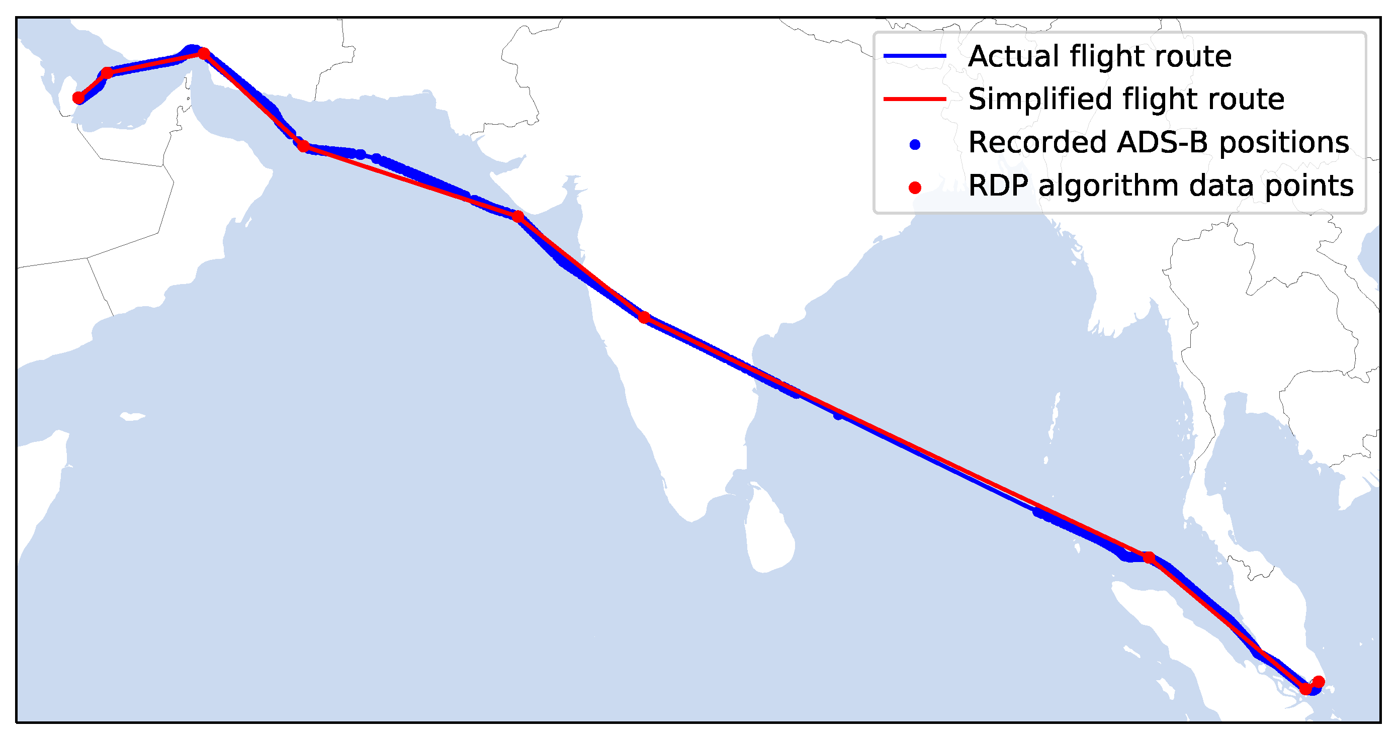
million data points, each representing a single received ADS-B message. The considered data points for a flight were reduced to necessary messages describing aircraft type, flight ID, position, altitude, speed and track. This data preparation aimed to provide input data to the flight performance model SOPHIA. Therefore, an Ramer-Douglas-Peucker (RDP) algorithm was applied for each recorded flight [
36]. The method separated the flight route recursively and kept the first and the last point of each segment. It then identified the distance between all points within the segment and an approximation line between the first and the last point of the segment. Each point of the segment was removed, since each point was closer than that which was within the distance
to the line segment, and the simplified curve could not be worse than
. The point furthest from the line segment had to be preserved if it was more than
from the approximation. The method called itself recursively with the first point and the farthest point and then with the farthest point and the last point, with the farthest point being noted as remaining in the process. When the recursion was finished, a new output curve could be constructed that contained only the points that were designated as maintained.
Figure 2 shows the result after simplifying the route of an example flight by using an
. The 476 blue dots represent the position of the aircraft based on the ADS-B messages. After the usage of the RDP algorithm, only the 9 red points were selected by the algorithm to describe the flown route with a reasonable level of accuracy. The use of this method reduced the number of data points by over 98% in this special case. Over 24.1 million data points were removed by the RDP algorithm, which also equals a reduction of over 98%.
3.1.2. Elaboration of Boundary Conditions for Speed and Route Control
To simplify the identification of the Target Time Over (TTO) reference point of the modelled trajectories, we determined a mean Top of Descent (TOD) for each flight from the historical data. Since the LR-ATFM concept should only be applied in the cruising phase of a flight, we assumed the position of the TOD, as transition between en-route and descent phase, to be the optimal and the latest possible TTO reference point along the flight route. The flight-specific TOD depends on the aircraft heading, wind speed and wind direction. To estimate the TOD location, the recorded altitude from ADS-B messages and the distance to WSSS were calculated based on the reported position information and the coordinates of WSSS were considered. For the determination of the TTO reference point distance to WSSS, only long-haul flights with a covered flight distance of at least 2200 NM were considered. Short- and medium-haul flights may be characterized by a short en-route phase in lower flight levels or they may have no en-route phase at all if the distance between the origin airport and WSSS is very short. Both possibilities would severely distort the determination of the TTO reference point.
Figure 3 (right) shows a lateral view of South East Asia with the transition area and a boundary line representing all TTO reference points 170 NM around WSSS. The area thus created is referred as the approach sector, shown in
Figure 3 (right). The flight is within the sector as soon as it crosses the TTO reference boundary (red circle in
Figure 3) and until it leaves the sector with its touch down on the runway. The optimization of the approach sector capacity utilization is the main target in the following analysis.
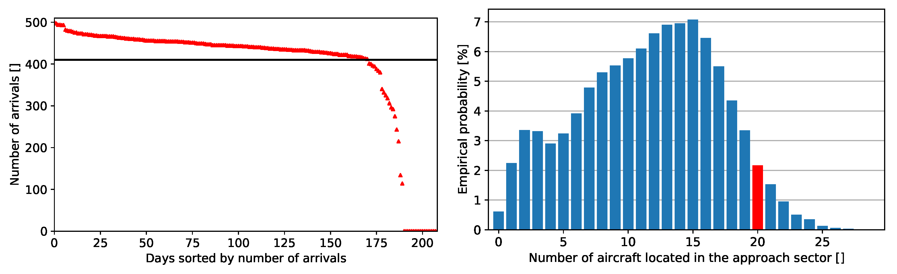
To define a capacity limit for the approach sector, a data-driven method using the ADS-B data was used.
Figure 4 (left) shows different days sorted by the number of arrivals in descending order. The peek value equals 500 arrivals followed by a steady moderate decrease to 410 arrivals. After this threshold value, the number of arrivals drops rapidly. The 38 days with less than 410 arrivals (below the black line) were excluded since these led to an underestimation of the approach sector capacity value. Reasons for the reduced number of flights are, e.g., data recording errors, severe weather or runway closures. For each of the remaining 171 days, the approach sector utilization was determined in five-minute time steps for the whole day and the number of aircraft located in the approach sector was counted.
Figure 4 (leftt) shows the distribution of the utilization values to determine the approach sector capacity. The most observed sector utilization values are between 13 and 15 aircraft. High utilization rates are synonymous with a high runway pressure at WSSS since all aircraft in the approach sector are funnelling to them. As a capacity value, the 95% quantile is defined, which equals 20 aircraft in the sector. In the following, this is called the
continuous capacity. If this threshold is exceeded, demand exceeds available resources and undesirable delays are a possible consequence. In this case, the LR-ATFM tries to shift the arrival times at the sector from long-haul flights using moderate speed or makes route changes to avoid exceeding the capacity limit. It should be noted that the actual capacity of the sector is likely to be underestimated as not all flights are equipped with ADS-B sensors, and therefore they do not appear in the data set, and some flights have been eliminated for various reasons.
3.1.3. Specification of the Period under Investigation
To show the impact of LR-ATFM on the approach sector capacity, a busy weekday (5 April 2019) with a high number of short and medium-haul arrivals was chosen to ensure a high base utilization in the approach sector. In addition, a traffic peak (
p.m. and
p.m.) of arriving long-haul flights was selected, to adjust the arrival time.
Figure 5 exhibits the utilization of the approach sector for the whole example day. The dashed blue line represents the utilization by short-and medium-haul flights, which are untouched by the LR-ATFM; therefore, the line is fixed. In the early hours until
a.m., the continuous capacity threshold is not touched by the curve. Thus, an overload does not occur during this period. In the afternoon hours, the capacity limit of the approach sector is already reached by non-controllable LR-ATFM flights in short periods. Therefore, each additional arrival in the approach sector leads to disadvantageous overload. The dashed orange curve in
Figure 5 represents the approach sector utilization by long-haul flights. Each flight has travelled more than 3100 NM to WSSS, ensuring a minimum cruising time of 5 h and thus a possible control of long-haul flights to WSSS as recommended by the ICAO, based on the results of a trial for the implementation of LR-ATFM [
37]. The orange line indicates the sum of all flights and represents the overall utilization of the approach sector. During the day, four major arrival peaks occur. Specifically, the congestion within the purple highlighted period between
p.m. and
p.m. (highlighted as dotted circle number II) occurs due to the impact of 26 long-haul flights. The other peaks (dotted circles I, III and IV) are majorly driven by short- and medium-haul flights. LR-ATFM aims to shift the arrival time of these flights at the approach sector to smooth the overall utilization curve and to avoid exceeding the continuous capacity. To ensure sufficient control time, LR-ATFM actions are performed in various scenarios
between 11 a.m.and 2 p.m., in half-hourly intervals, to determine the most suitable time for interventions.
If the arrival time at the approach sector is modified by LR-ATFM activities, compared to the historic flights, the time spent within the approach sector may change as well due to different traffic conditions within the approach sector. Therefore, an assumption for the time aircraft spent in the approach sector for LR-ATFM regulated flights is specified based on the time distribution of the historic flight data, which is shown in
Figure 6. The most frequent observed flight time within the approach sector is around 35 min. Higher flight times are possible for holdings or inefficient arrival routes, which leads to a right skew of
Figure 6. The box plot underlines the statement since the time difference between the 25% quantile and lower whisker is three times lower compared to the time difference between the upper whisker and 75% quantile. Since the example day represents a busy weekday, we decided to assume a flight time within the approach sector similar to the 75% quantile (40:25 min) for regulated long-haul flights.
3.2. Identification of Alternative Routes for Scenarios
Usually, each flight has several route options to reach the destination from the origin airport. The options are defined by way points connected via Air Traffic System (ATS) routes flown consecutively. To extract possible route options based on historical data and the current aircraft position, a two step approach is applied for 18 long-range origin and destination connections covering all 26 long-haul flights. The procedure is explained in
Figure 7 using flight QTR946 from Doha Hamad International Airport (OTHH) to WSSS.
The route network is defined by recorded ADS-B flights between the considered origin airport and WSSS. In the case of flight QTR946, 481 flights between OTHH and WSSS are provided by the data set. For each flight, the route is simplified and divided into 16 segment positions based on the total flight time (see Step 1 in
Figure 7). The first position is placed on the origin airport and the last position corresponds to a position 30 min before reaching the approach sector. The grey box in
Figure 7 includes the position for segment III which will be considered in more detail below. Simplifying each flight path into a constant number of positions allows a clustering of each individual segment. Step 2 in
Figure 7 shows all 481 positions for segment III. For this purpose, a kernel density estimation (KDE) is performed based on the angular positions of all segment points to WSSS (Step 3 in
Figure 7). A KDE allows for the estimation of the density using a non-parametric approach. Since the angle is a circular measure with a transition at 360 degrees, a Gaussian kernel with periodic conditions is chosen. The selected bandwidth of the kernel is set to 1.15 degrees. The number of peaks of the resulting convoluted distribution defines the number of clusters for a segment. The angle boundaries between a cluster equals the corresponding minimum values (highlighted as a black line). Subsequently, each segment point is assigned to its cluster based on the boundaries. For each cluster, a weighted centre (red points) is evaluated, which considers the location of all cluster points (Step 4 in
Figure 7). In the subsequent procedure, the cluster centres are assumed to be representative of the actual aircraft segment position. The connection of all 16 extracted cluster centres for each segment results in the generalized route for a flight (Step 5 in
Figure 7). The complete route network consists of all extracted simplified flight routes (Step 6 in
Figure 7). If more than three possible alternative routes per flight and per scenario
could be extracted, we manually chose three of them, considering a perceptible lateral difference with a maximum diversion of 8%.
3.3. Airport Capacity Optimization
In this section, we will introduce mathematical modelling, which will be used to identify the ideal solution and combination of flight options to minimize the fuel consumption for all flights during the entire period of optimization.
| Sets: |
| T | set of time steps in the optimization horizon |
| I | set of all flights |
| Ji | set of all options for flight i |
| Parameters: |
| The amount of fuel burn by j-th option of flight i |
| The already used capacity by short- and medium-haul flights at time t based on the real situation |
| U | The constant capacity of approach sector over all time steps |
| M | A parameter defining big M |
| The binary parameter, 1 if the j-th option of flight i is in the approach sector at time t, and 0 otherwise |
| Variables: |
| binary variable—equal to 1 if for flight i its j-th option is chosen, and 0 otherwise |
| integer variable—the amount of violation of the capacity at time t |
The objective function of the problem, as defined by Equation (1), is to discover the flying option that consumes the least amount of fuel. The first component of the function is responsible for this, while the second part of the function attempts to prevent the model from deviating from the stated capacity to the extent that it is practical. Constraint (2) guarantees that the number of flights in the approach sector does not exceed the amount of capacity that has been pre-assigned at the time t. If it becomes impossible to find a solution to the problem, we may relax the constraint by considering the variable , which represents the number of flights that would be accepted if it became impossible to fit all flights into the available capacity. Constraint (3) ensures that one (and only one) option for each flight is selected in the optimal solution. Constraint (4) defines the variable types.
3.4. Flight Performance Modelling
The aircraft performance model SOPHIA is used to calculate the impact of arrival time manipulation on fuel burn. Furthermore, calculating the flight performance of each manipulation ensures that only physically possible trajectories are considered in the optimization of the arrival time. The flight performance model SOPHIA calculates and optimizes only physically possible 4-D aircraft trajectories and is validated for 16 different aircraft types [
38,
39]. In SOPHIA, the equation of motion is solved analytically (except for the drag polar, which is approximated by the OpenAP model [
32]). The model differs from other aircraft performance models in the consideration of the forces of acceleration and inertia each time step by a Proportional–Integral–Derivative (PID) controller which controls the true airspeed and uses the lift coefficient as a regulative variable. The parameters of the controller are aircraft type specific. The aircraft type-specific behaviour, modelled with SOPHIA, has been demonstrated in [
33,
40].
For flight performance modelling following a historic, fully defined flight, the cruising altitude and the true airspeed are effective variables provided by the ADS-B data. For trajectory manipulation speed, path and altitude are provided as target functions to a PID controller which controls the lift coefficient to achieve the aspired speed and altitude. Flight performance modelling is highly sensitive to aircraft mass assumptions which are not provided by ADS-B data. Here, we consider an Operational Empty Weight (OEM), payload and fuel load as aircraft’s mass components. To calculate the payload, we use a seat load factor of
, an average passenger weight of 77 kg plus
kg luggage per passenger [
41]. The OEM and an average aircraft seating per aircraft type are derived from aircraft manuals for airport planning (e.g., [
42] for the A320). Trip fuel is estimated iteratively and
contingency fuel and holding fuel (a 30 min flight at
feet altitude at a speed for a maximum lift to drag ratio, computed with SOFIA) make up the fuel load [
39].
SOPHIA contains a combustion chamber model to quantify the emissions as products of complete combustion (e.g., , and ) and incomplete combustion (e.g., , , and black carbon) and to quantify the fuel burn.
3.4.1. Speed Adjustments in Scenarios
In each scenario
, we manipulate the aircraft speed at a specific
and therewith we manipulate the arrival time and the fuel burn. Starting from a typical cruising speed specified in aircraft characteristics, this speed is increased and decreased in steps of
Mach = 0.01 until aircraft type-specific and weather-specific flight performance limits are reached. These limits refer on the one hand to the stall speed
, which represents an equilibrium in the vertical direction for a given mass, and on the other hand to the Mach
max which is tabulated in aircraft characteristics.
Figure 8 exemplifies the calculated impact of speed manipulation on fuel burn and arrival time of a B777 flight from Paris Charles de Gaulle LFPG to WSSS. In this case, we started the speed manipulation at 11.00 a.m., 12.30 a.m. and 2.00 p.m. The reference cruising conditions are highlighted in red. Within the remaining 4.5 h of flight time, the arrival time could be shifted forwards and backwards by about 30 min.
3.4.2. Route Adjustments
LR-ATFM can include more than speed adjustments. At certain times
, alternative routes
might additionally be available, which also manipulate the arrival time. For this reason, as described in
Section 3.2, alternative historical routes were extracted and assigned to corresponding times
. In scenarios
, the flight performance along the alternative routes was modelled and additionally subjected to all speed adjustments.
Figure 9 gives an example of three different routes of an A330 flight QTR946 from OTHH to WSSS. We thus increase the potential of arrival time optimisation to about the same order of magnitude as with the speed adjustments. Earlier arrivals result in a similar effect on fuel consumption, as speed increases. In contrast to speed reductions (and resulting fuel burn reductions), later arrivals due to detours result in fuel increases. Note, depending on the aircraft distance to WSSS at time
, greater or fewer alternative routes are available. For
= 11 a.m. at least one alternative route was available for 25 flights. At 12.30 a.m., 11 flights still had the possibility to change their route. At 2 p.m., an alternative route was available for only a single flight, QTR946.
4. Potential of LR-ATFM in the South-Pacific Region
Due to the limited number of long-haul flights between 3 p.m. and 6 p.m. on the day of investigation, 5th April 2019, we could solve the NP-hard model using common solvers without needing to use a metaheuristic. Among the provided input arrival times with corresponding fuel burns, the optimizer was able to reduce the number of time steps with airspace utilization exceeding the capacity of 20 simultaneous aircraft in the approach sector.
4.1. Potential of Speed Adjustments on LR-ATFM
To investigate the impact of both methods for manipulating the arrival time separately, we initially only provided speed adjusted arrival times and fuel burns to the optimizer. The mathematical model was solved using Gurobi package 8.0 on a 24-kernel CPU with 32 GB RAM on Windows 10. Route options were added later in
Section 4.2. As derived in
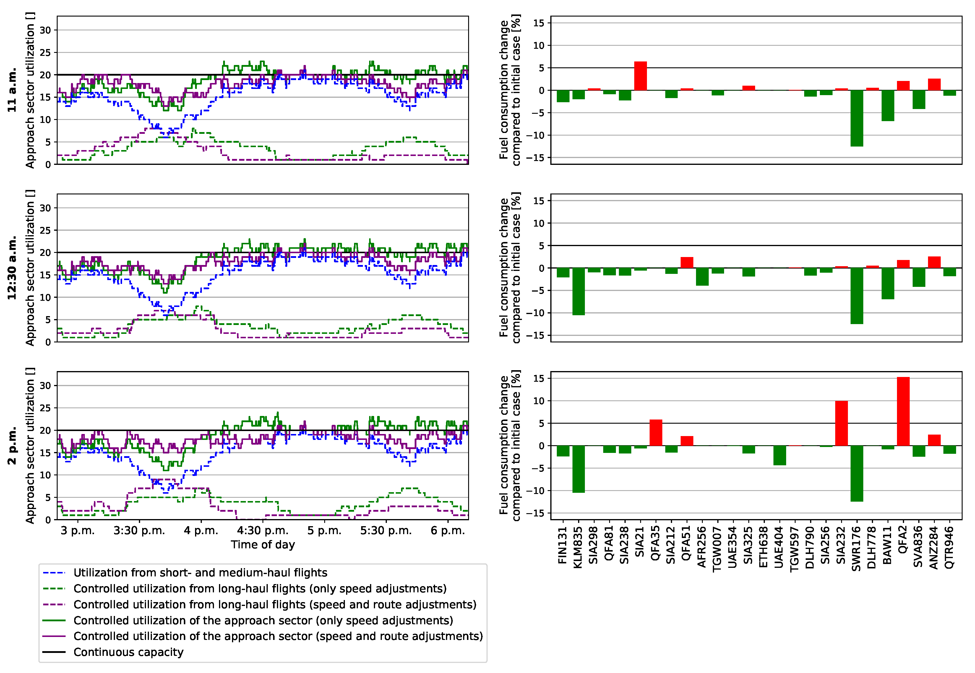
Section 3.4.1, the impact of speed adjustments on the arrival time depends on the remaining flight time until TTO and amounts to a maximum of one hour. The method turned out to be effective and necessary, as speed adjustments were not made for all flights (
Figure 10). As expected, the earlier the speed is interfered with, the more effectively the arrival time can be manipulated. From this it follows that, with
= 11.00 a.m., both the additional fuel burn and the maximum utilization are minimized (see solid green line in
Figure 10, top). However, during this busy peak time, a target sector capacity of 20 aircraft could not be reached. The uncontrolled maximum utilization (i.e., max. 32 aircraft, see the orange curved line in
Figure 10) could be flattened to a maximum of 23 aircraft. For
= 11.00 a.m., there is a significant violation from 4.15 p.m. to 5:15 p.m. for one hour (orange line in
Figure 10), which is smoothed out after optimization to have the violation for a longer period but not a significant uncontrolled violation. However, the method extends the period with utilisation greater than 20 aircraft in the sector (from ≈ one hour to ≈ two hours with some interruptions, see also
Table 1). The shorter the time to TTO (i.e.,
11.00 a.m.), the higher the fuel investigation for reaching a balanced distribution of long-haul arrivals in the approach sector and the longer the approach sector is overloaded. Despite this, even ≈ one hour before TTO (i.e.,
= 2 p.m.), the optimizer found speed manipulated solutions to decrease the utilization peaks in the approach sector by holding off on flights, although with higher fuel investigation. Considering a relationship between arrival time and fuel burn as shown in
Figure 8 for all flights, the optimizer preferred increased speed and increased fuel (red bars in
Figure 10) instead of decreased speed and fuel saving (green bars in
Figure 10).
The advantage of this method of controlling the arrival time in the approach sector is a low organisational effort since speed adjustments during cruising of plus/minus
are allowed without Air Traffic Control (ATC) clearance [
43].
4.2. Potential of Alternative Routes on LR-ATFM under Real Weather Conditions
Besides speed adjustments, lateral route changes may be an alternative to control the arrival time, as soon as the aircraft is in the air. For small deviations from the initially filed route, the impact of this option on fuel burn depends on the weather conditions. The longer the diversion, the higher the probability of increased fuel burn and the higher the potential to shift the arrival time at the approach sector. When providing arrival times of alternative routes and corresponding fuel burns to the optimizer, the potential of LR-ATFM is significantly higher. Specifically, the total fuel burn could be decreased. The maximum utilization could be minimized to 22 flights and the sector overload time could be decreased significantly by more than one hour. Since even one hour before TTO, at least one alternative route could be identified for most of the flights (compare
Section 3.2 for details), LR-ATFM with alternative routes can be effective even within a short period. The combination of speed and route adjustments enabled us to minimize the approach sector utilization. In this case study, the (weather-dependent) fuel burn benefit was at a maximum, when adjusting speed and route
h before arrival (i.e.,
a.m.). However, the result could be different on another day with different weather conditions.
4.3. Optimal Time Frame of LR-ATFM
The research aim of this study was to identify the optimal time before arrival for an effective LR-ATFM. Considering only speed adjustments, the sooner the control takes place, the more fuel-efficient the arrival time could be. Thereby, small deviations from the optimal cruising speed over a long period are more fuel-efficient than large speed adjustments over a short period (see
Table 1). However, the sooner the control starts, the more difficult the prediction of the arrival time is, since weather conditions are difficult to predict. For this reason, we did not expand the starting time to
a.m. Allowing for route changes significantly increases the flexibility of the LR-ATFM (see
Figure 11). Even with an intervention in the ATM one hour before arrival, we were able to reduce the overload time by ≈90%, although a maximum of three different routes per flight were allowed (as shown in
Table 1, bottom). Assuming a successful weather prediction of two to four hours (either by reports of aircraft flying ahead or by numerical weather prediction models), we advise starting with an LR-ATFM about four hours in advance. If further route adjustments are allowed and possible, we advise that one should prefer this option one to two hours before the TOD.
5. Conclusions
In this study, we investigated the potential to control 26 long-haul flights during cruise by applying speed adjustments and alternative routes to harmonize the number of aircraft in the approach sector of WSSS. During the peak hour of a busy day, we could not reach our goal of keeping the sector utilization below 21 simultaneous aircraft in the sector. The best solution (22 aircraft at the same time, instead of 32) was achieved by allowing speed adjustments and alternative routes for all chosen starting times . We could solve the optimization as an NP-hard problem with acceptable calculation time. For larger networks, the implementation of metaheuristic algorithms will be necessary to find the optimal solution. We concentrated on controlling the cruise phase because we wanted to relieve the approach sector by limiting the number of flights within this airspace. Although the descent phase might have huge potential to manipulate the arrival time on the Final Approach Fix (FAF), the approach sector is already burdened by dense traffic patterns and increased complexity.
We found it necessary to calculate the flight performance of each flight individually since weather conditions and different optimal cruising speeds of each flight greatly affect the arrival time. Specifically, the impact of alternative routes on fuel burn is hard to predict. In this first performance-based study of LR-ATFM, we neglected airport operations, such as the runway occupancy time and the utilization of the taxiway and apron system. These tasks of the AMAN should be considered in the following study. Furthermore, departures at the airport of interest should be considered intensively. The current optimization procedure only focuses on arrivals. Right now, a possible runway utilization of the departing aircraft is unknown to the optimizer and might be used for arrivals. In this case, an AMAN was included in our optimization. The optimization of the descent phase might be a promising option to reduce fuel burn and to control the arrival time. Additionally, future scientific work should focus on maximum additional fuel consumption of , as this corresponds to the planned contingency fuel of a flight.
To reduce the ATFM problem to a well-defined task, we did not allow changes of the vertical profile (i.e., flight levels, step climb, descent steps). In the case of route adjustments, we simply calculated an optimal TOD position, i.e., during detours, we let the aircraft fly at its last defined cruising altitude. Changes and optimizations of the vertical profile would generate lots of conflicts with surrounding aircraft.
One of our main findings concentrates on scenarios , where only speed adjustments are allowed. We found that the earlier the control takes place, the more efficient LR-ATFM can be. This might lead to the idea of a controlled ground holding program at the departure airport. However, the coupling of different departure airports with arrival airports increases the complexity of the optimization problem. The resulting number of free variables might result in an unsolvable optimization problem, especially because the arrival time of long-haul flights under real weather conditions is hard to predict.
The promising potential of alternative routes at any time for both harmonized arrival time and fuel burn motivates us to also consider medium-haul flights in future publications of our LR-ATFM program. Furthermore, a wind-optimized (maybe waypoint-less) route might be a welcome alternative.
Author Contributions
Conceptualization: J.R.; methodology: J.R., E.A., D.L., software: J.R., E.A., D.L. validation: J.R., E.A., D.L., formal analysis: J.R., E.A., D.L., investigation: J.R., E.A., D.L., M.S., resources: J.R., data curation: J.R., D.L., writing–original draft preparation: J.R., E.A., D.L. writing–review and editing: J.R., E.A., D.L., visualization: J.R., E.A., D.L., supervision: J.R., H.F. project administration: J.R., funding acquisition: J.R., H.F. All authors have read and agreed to the published version of the manuscript.
Funding
This research is financed by Deutsche Forschungsgemeinschaft (DFG, German Research Foundation) in the framework of the project UBIQUITOUS-410540389 and German Federal Ministry for Economic Affairs and Climate Action (BMWK) within the LUFO-V grant agreement No. 20X1711M (OPsTIMAL).
Institutional Review Board Statement
Not applicable.
Informed Consent Statement
Not applicable.
Acknowledgments
The authors would like thank the reviewers for valuable comments.
Conflicts of Interest
The authors declare no conflict of interest.
References
- ICAO. Annex 11—Air Traffic Services, 15th ed.; ICAO: Montreal, QC, Canada, 2018. [Google Scholar]
- ICAO. DOC 9750—Global Air Navigation Plan, 6th ed.; ICAO: Montreal, QC, Canada, 2019. [Google Scholar]
- “PANS-ATM, Procedures for Navigation Services—Air Traffic Management,” Doc 4444, 16th ed.; International Civil Aviation Organization: Montreal, QC, Canada, 2016.
- EUROCONTROL Network Manager. ATFCM Users Manual, Edt. 22.1; EUROCONTROL: Brussels, Belgium, 2018. [Google Scholar]
- EUROCONTROL Airport CDM Team. Airport CDM Implementation Manual, Ver. 5; EUROCONTROL: Brussels, Belgium, 2017. [Google Scholar]
- FAA. Traffic Flow Management in the National Airspace System; FAA: Washington, DC, USA, 2009. [Google Scholar]
- Tanino, M. FAA Experiences with ATFM. In Proceedings of the ACAO/ICAO Air Traffic Flow Management Workshop, Casablanca, Morocco, 17–18 March 2019. [Google Scholar]
- ICAO. Asia/Pacific Regional Air Traffic Flow Management Concept of Operations, v1.0; ICAO: Montreal, QC, Canada, 2015. [Google Scholar]
- Guillet, R. NARAHG Northeast—Asia Regional ATFM Harmonization Group. In Proceedings of the ICAO ATFM Global Symposium (ATFM2017), Singapore, 20–22 November 2017. [Google Scholar]
- González-Arribas, D.; Soler, M.; Sanjurjo-Rivo, M.; García-Heras, J.; Sacher, D.; Gelhardt, U.; Lang, J.; Hauf, T.; Simarro, J. Robust Optimal Trajectory Planning Under Uncertain Winds and Convective Risk. In Air Traffic Management and Systems III; Electronic Navigation Research Institute, Ed.; Springer: Singapore, 2019; pp. 82–103. [Google Scholar]
- Xu, Y.; Prats, X.; Delahaye, D. Synchronised demand-capacity balancing in collaborative air traffic flow management. Transp. Res. Part C Emerg. Technol. 2020, 114, 359–376. [Google Scholar] [CrossRef] [Green Version]
- Kistan, T.; Gardi, A.; Sabatini, R.; Ramasamy, S.; Batuwangala, E. An evolutionary outlook of air traffic flow management techniques. Prog. Aerosp. Sci. 2017, 88, 15–42. [Google Scholar] [CrossRef]
- ICAO. DOC 9971—Manual on Collaborative Air Traffic Flow Management (ATFM), 3rd ed.; ICAO: Montreal, QC, Canada, 2018. [Google Scholar]
- Gwiggner, C.; Nagaoka, S. Sequencing Strategies for a Japanese Arrival Flow. In Proceedings of the 9th AIAA Aviation Technology, Integration, and Operations Conference, Hilton Head, SC, USA, 21–23 September 2009. [Google Scholar]
- Jones, J.C.; Lovell, D.J.; Ball, M.O. Stochastic Optimization Models for Transferring Delay Along Flight Trajectories to Reduce Fuel Usage. Transp. Sci. 2018, 52, 134–149. [Google Scholar] [CrossRef]
- Prats, X.; Hansen, M. Green Delay Programs: Absorbing ATFM Delay by Flying at Minimum Fuel Speed. In Proceedings of the 9th USA/Europe Air Traffic Management Research and Development Seminar, Berlin, Germany, 14–17 June 2011. [Google Scholar]
- Dhief, I.; Lim, Z.J.; Goh, S.K.; Pham, D.T.; Alam, S.; Schultz, M. Speed Control Strategies for E-AMAN using Holding Detection-Delay Prediction Model. In Proceedings of the 10th EUROCONTROL SESAR Innovation Days, Brussels, Belgium, 7–10 December 2020. [Google Scholar]
- Schultz, M.; Lubig, D.; Asadi, E.; Rosenow, J.; Itoh, E.; Athota, S.; Duong, V.N. Implementation of a Long-Range Air Traffic Flow Management for the Asia-Pacific Region. IEEE Access 2021, 9, 124640–124659. [Google Scholar] [CrossRef]
- Buffa, E.S.; Cosgrove, M.J.; Luce, B.J. An integrated work shift scheduling system. Decis. Sci. 1976, 7, 620–630. [Google Scholar] [CrossRef]
- Bhulai, S.; Koole, G.; Pot, A. Simple methods for shift scheduling in multiskill call centers. Manuf. Serv. Oper. Manag. 2008, 10, 411–420. [Google Scholar] [CrossRef]
- Rekik, M.; Cordeau, J.F.; Soumis, F. Implicit shift scheduling with multiple breaks and work stretch duration restrictions. J. Sched. 2010, 13, 49–75. [Google Scholar] [CrossRef]
- Shuib, A.; Kamarudin, F.I. Solving shift scheduling problem with days-off preference for power station workers using binary integer goal programming model. Ann. Oper. Res. 2019, 272, 355–372. [Google Scholar] [CrossRef]
- Asadi, E.; Schultz, M.; Fricke, H. Optimal schedule recovery for the aircraft gate assignment with constrained resources. Comput. Ind. Eng. 2021, 162, 107682. [Google Scholar] [CrossRef]
- Tello, F.; Jiménez-Martín, A.; Mateos, A.; Lozano, P. A comparative analysis of simulated annealing and variable neighborhood search in the ATCo work-shift scheduling problem. Mathematics 2019, 7, 636. [Google Scholar] [CrossRef] [Green Version]
- Álvarez, E.; Ferrer, J.C.; Muñoz, J.C.; Henao, C.A. Efficient shift scheduling with multiple breaks for full-time employees: A retail industry case. Comput. Ind. Eng. 2020, 150, 106884. [Google Scholar] [CrossRef]
- Eurocontrol Experimental Center. Coverage of European Air Traffic by Base of Aircraft Data (BADA), Revision 3.6 ed.; Eurocontrol: Brussels, Belgium, 2004. [Google Scholar]
- User Manual for the Base of Aircraft Data (BADA) Family 4; Eurocontrol: Brussels, Belgium, 2012.
- Poles, D.; Nuic, A.; Mouillet, V. Advanced aircraft performance modeling for ATM: Analysis of Bada model capabilities. In Proceedings of the 29th Digital Avionics Systems Conference, Salt Lake City, UT, USA, 3–7 October 2010. [Google Scholar]
- Calders, P. G.A.M.E. Aircraft Performance Model Description. In DIS/ATD Unit, DOC.CoE-TP-02002; EUROCONTROL: Brussels, Belgium, 2002. [Google Scholar]
- Calders, P. Getting to grips with Aircraft Performance. Flight Oper. Support Line Assist. 2002, 2, 11–16. [Google Scholar]
- Simos, D. PIANO: PIANO User’s Guide Version 4.0; Lissys Limited: London, UK, 2004. [Google Scholar]
- Sun, J.; Hoekstra, J.; Ellerbroek, J. OpenAP: An Open-Source Aircraft Performance Model for Air Transportation Studies and Simulations. Aerospace 2020, 7, 104. [Google Scholar] [CrossRef]
- Rosenow, J.; Fricke, H. Flight performance modeling to optimize trajectories. In Proceedings of the Deutscher Luft- und Raumfahrtkongress 2016, Braunschweig, Germany, 13–15 September 2016. [Google Scholar]
- Lindner, M.; Rosenow, J.; Fricke, H. Dynamically Optimized Aircraft Trajectories Affecting the Air Traffic Management. In Proceedings of the 8th International Conference on Research in Air Transportation, Barcelona, Spain, 26–29 June 2018. [Google Scholar]
- Lindner, M.; Rosenow, J.; Zeh, T.; Fricke, H. In-flight aircraft trajectory optimization within corridors defined by ensemble weather forecasts. In Proceedings of the International Conference on Research in Air Transportation (ICRAT), Online, 15 September 2020. [Google Scholar]
- Douglas, D.; Peucker, T. Algorithms for the reduction of the number of points required to represent a line or its caricature. Can. Cartogr. 1973, 10, 112–122. [Google Scholar] [CrossRef] [Green Version]
- ICAO. Long range ATFM concept trials. In Proceedings of the 8th Meeting of the Asia/Pacific ATFM Steering Group (ATFM/SG/8), New Delhi, India, 14–18 May 2018. [Google Scholar]
- Rosenow, J.; Chen, G.; Fricke, H.; Sun, X.; Wang, Y. Impact of Chinese and European Airspace Constraints on Trajectory Optimization. Aerospace 2021, 8, 338. [Google Scholar] [CrossRef]
- Rosenow, J.; Chen, G.; Fricke, H.; Wang, Y. Factors impacting Chinese and European Vertical Fight Efficiency. Aerospace 2022, 9, 76. [Google Scholar] [CrossRef]
- Rosenow, J.; Förster, S.; Fricke, H. Continuous Climb Operations with minimum fuel burn. In Proceedings of the Sixth SESAR Innovation Days, Delft, The Netherlands, 8–10 November 2016. [Google Scholar]
- Berdowski, Z.; van den Broek-Serlé, F.; Jetten, J.; Kawabata, Y.; Schoemake, J.T.; Versteegh, R. Survey on Standard Weights of Passengers and Baggages. EASA 2008.C.06/30800/R20090095/30800000/FBR/RLO. 2009. Available online: https://www.easa.europa.eu/sites/default/files/dfu/Weight%20Survey%20R20090095%20Final.pdf (accessed on 20 February 2022).
- AIRBUS, S.A.S. A320/A320NEO Aircraft Characteristics, Airport and Maintenance planning. In Technical Report, AIRBUS S.A.S Customer Services Technical Data Support and Service; Airbus S.A.S.: Blagnac, France, 2014. [Google Scholar]
- Rosenow, J.; Lindner, M.; Scheiderer, J. Advanced Flight Planning and the Benefit of In-Flight Aircraft Trajectory Optimization. Sustainability 2021, 13, 1383. [Google Scholar] [CrossRef]
Figure 1.
An example of a work shift scheduling problem.
Figure 1.
An example of a work shift scheduling problem.
Figure 2.
Simplification of an example flight route using the RDP algorithm with .
Figure 2.
Simplification of an example flight route using the RDP algorithm with .
Figure 3.
Left: TTO reference point distance to WSSS. Right: Lateral view of the approach sector (170 NM around WSSS).
Figure 3.
Left: TTO reference point distance to WSSS. Right: Lateral view of the approach sector (170 NM around WSSS).
Figure 4.
Left: Number of arriving flights at WSSS. Right: Approach sector capacity determination.
Figure 4.
Left: Number of arriving flights at WSSS. Right: Approach sector capacity determination.
Figure 5.
Approach sector utilization during the example day (5 April 2019), based on historic data.
Figure 5.
Approach sector utilization during the example day (5 April 2019), based on historic data.
Figure 6.
Left: Distribution of flight time within the approach sector to WSSS. Right: Corresponding box plot with median, 25% and 75% quantile (red line) as well as the whiskers located at the 1% and 99% quantile.
Figure 6.
Left: Distribution of flight time within the approach sector to WSSS. Right: Corresponding box plot with median, 25% and 75% quantile (red line) as well as the whiskers located at the 1% and 99% quantile.
Figure 7.
Evaluation of a generalized route network based on historic flight data.
Figure 7.
Evaluation of a generalized route network based on historic flight data.
Figure 8.
Fuel burn and arrival time of a B777 flight AFR256 from Paris Charles de Gaulle to WSSS. Cruising speed is changed from = 11.00 a.m. (black), = 12.30 a.m. (green) and = 2.00 p.m. (blue) between Mach 0.7 and 0.86 in steps of Mach = 0.01. The red cross indicates the reference cruising conditions with Mach 0.8.
Figure 9.
Three different lateral routes for A330 flight QTR946 from OTHH to WSSS. The route was changed from = 11:00 a.m. Black: original route with arrival time at 3:55 p.m. and fuel burn 37,182 kg. Blue: first alternative arriving at 4:18 p.m. with 37,976 kg fuel burn. Red: second alternative arriving at 3:14 p.m. with 36,154 kg fuel burn. Without any speed adjustments, arrival times could be adjusted by 50 min with differences in fuel burn of kg.
Figure 10.
Left: Optimization results using LR-ATFM with speed adjustments. Right: Fuel change compared between the use of LR-ATFM with speed adjustments and the initial case with no LR-ATFM usage.
Figure 10.
Left: Optimization results using LR-ATFM with speed adjustments. Right: Fuel change compared between the use of LR-ATFM with speed adjustments and the initial case with no LR-ATFM usage.
Figure 11.
Left: Optimization results using LR-ATFM with speed and route adjustments compared to the optimization results using LR-ATFM with only speed adjustments. Right: Fuel change compared between the usage of LR-ATFM with speed and route adjustments to the initial case with no LR-ATFM usage.
Figure 11.
Left: Optimization results using LR-ATFM with speed and route adjustments compared to the optimization results using LR-ATFM with only speed adjustments. Right: Fuel change compared between the usage of LR-ATFM with speed and route adjustments to the initial case with no LR-ATFM usage.
Table 1.
Impact of Long-haul speed adjustments and route changes during cruising on a balanced distribution of arrivals to WSSS. The sooner speed adjustments take place, the smaller the approach sector overload. Alternative routes (WR) enable aircraft to both shift the arrival time and save fuel.
Table 1.
Impact of Long-haul speed adjustments and route changes during cruising on a balanced distribution of arrivals to WSSS. The sooner speed adjustments take place, the smaller the approach sector overload. Alternative routes (WR) enable aircraft to both shift the arrival time and save fuel.
| LR-ATFM Intervention Time | 11 a.m. | 11:30 a.m. | 12 a.m. | 12:30 a.m. | 1 p.m. | 13:30 p.m. | 14 p.m. |
|---|
| NR | WR | | | NR | WR | | | NR | WR |
|---|
| Number of controllable LR flights | 26 | 26 | 26 | 26 | 26 | 26 | 25 | 23 | 23 | 23 |
Approach sector overload
between 2:50 p.m. and 6:10 p.m. [hh:mm:ss]
-change against initial case [%]) | 00:50:58
(−21.2) | 00:06:25
(−90.1) | 00:49:56
(−22.8) | 01:02:37
(−3.2) | 01:06:50
(+3.4) | 00:07:07
(−89) | 01:14:42
(+15.5) | 01:14:44
(+15.6) | 01:08:19
(+5.6) | 00:07:03
(−89.1) |
| Utilization peak in approach sector | 23 | 22 | 23 | 23 | 23 | 22 | 23 | 24 | 24 | 22 |
| Number of speed changes | 19 | 12 | 20 | 21 | 22 | 12 | 21 | 19 | 19 | 15 |
| Number of route changes | - | 16 | - | - | - | 14 | - | - | - | 8 |
Number of flights
with fuel benefit | 7 | 12 | 8 | 10 | 9 | 16 | 9 | 9 | 8 | 14 |
Number of flights delayed
by more than 15 min | 10 | 6 | 13 | 13 | 13 | 10 | 12 | 11 | 11 | 11 |
Sum of overall fuel consumption diffe-
rence compared to the initial case [kg] ([%]) | +4701
(+0.3) | −19,541
(−1.4) | +11,090
(+0.8) | +5837
(+0.4) | +3278
(+0.2) | −37,619
(−2.7) | +1742
(+0.1) | +4678
(+0.4) | +4685
(+0.4) | −6235
(−0.5) |
| Publisher’s Note: MDPI stays neutral with regard to jurisdictional claims in published maps and institutional affiliations. |
© 2022 by the authors. Licensee MDPI, Basel, Switzerland. This article is an open access article distributed under the terms and conditions of the Creative Commons Attribution (CC BY) license (https://creativecommons.org/licenses/by/4.0/).


