1. Introduction
During the year 2020, COVID-19 spread rapidly around the world and evolved into a worldwide pandemic. The impact of COVID-19 is nowadays visible in many business sectors. Governments implemented measures to reduce the risk of contamination by, for example, shutting down business sectors, implementing travel restrictions, or supporting home offices [
1,
2]. This change in the world heavily affects public transport services. Due to regulations and changes in travel habits, the number of weekly household trips was reduced by 50%, and the mode share of public transport was reduced from 15% to 7% during the lockdown period in Australia [
3]. The demand reduction in Colombia was around 80% to 90%, with the highest demand loss of 96% observed in Cartagena during their mandatory quarantine period [
4]. This demand reduction was also around 90% in the Netherlands [
5], and the same trend has been observed in major cities in China, Iran, and the U.S. [
6]. Some public transport operators in the United Kingdom also reported a decrease of as much as 70% [
7].
Public transport operators are not only affected by the lower travel demand; their operations should also conform with the government regulations relating to COVID-19 [
8]. These regulations consist mostly of wearing a face mask and physical distancing [
9,
10,
11]. The latter regulation implies that in-vehicle capacities are reduced to pandemic-imposed capacities.
In a post-lockdown period, some activities will resume and will result in an increase in passenger demand. This will force public transport operators to apply physical distancing measures to reduce the virus transmission risk. Tirachini and Cats [
12] stated that there are some options to avoid exceeding the pandemic-imposed capacity of vehicles. These options are managing the limited capacity, redesigning public transportation services, crowd management, or passenger demand spreading.
This study focuses on public transport services in a post-lockdown period, where demand may exceed the pandemic-imposed capacity at some sections of the service lines. In particular, we consider short-turning strategies as it might be efficient for public transport operators to increase frequencies for some heavily crowded line segments [
13]. The goal is to develop a frequency setting model on a tactical level that distributes the available vehicles over original lines and short-turning sublines while considering the pandemic-imposed capacity. The frequency setting model is tested on two high-demand bus lines in the region of Twente, the Netherlands. The model should help to answer the following research question:
The remainder of the paper is organized as follows.
Section 2 reviews the literature related to the public transport frequency settings problem.
Section 3 describes the methodology, including models for the worst-case and best-case scenarios. In
Section 4, the case study will be presented and the model will be tested. This section also analyzes the results of the model’s application.
Section 5 concludes the paper and provides future research directions.
2. Literature Review
Maintaining social distancing can be achieved by means of a combination of measures. At the strategic level, decisions about the modification of public transport stops (e.g., stop closures) have been implemented [
14]. Transport for London and Washington Metro are just two of the public transport authorities/service providers that decided to close specific public transport stations to avoid overcrowding beyond the COVID-19 capacity limit. Other measures in this direction include the suspension of public transport services during the late afternoon or evening hours [
15]. Another long-term measure could be increasing the fleet size by purchasing more public transport vehicles in order to ensure that we have sufficient service supply even during peak times [
16].
At the tactical planning level, the decisions are focused on short-term planning and can include the change in service frequencies, the change in service patterns, modifications of vehicle/crew schedules, and timetable adjustments [
12,
17]. Despite the changes at the strategic or tactical planning stage, unforeseen demand variations during the actual operations might require the adoption of extra control measures, such as the skipping of stops or the refusal of passenger boardings. During the first pandemic wave in the UK, bus drivers were allowed to skip public transport stops or refuse boardings once their buses reached their pandemic-imposed capacity [
6]. From this spectrum of potential social distancing control measures, our study will focus on short-term planning measures that consider the modification of service frequencies considering a fixed number of available vehicles.
The problem of finding optimal frequency settings can be defined as the transit network frequency setting problem, where the goal is to find the optimal frequencies over a time period given a passenger demand and a set of transit network routes [
18,
19,
20,
21]. Early approaches to determine the optimal frequency for a single line are the square root rule [
22,
23,
24], where the frequency is proportional to the square root of the ratio between the waiting costs and operational costs, and the maximum loading point method [
25,
26]. The latter method determines optimal frequencies based on the load profiles and maximum load points along a route.
More complex models determine the optimal frequency and allocation of vehicles over multiple lines (e.g., Schéele [
27], Furth and Wilson [
28], Constantin and Florian [
29). Schéele [
27] solved the trip assignment and the frequency setting problems simultaneously. Furth and Wilson [
28] considered fleet size constraints, budget and headway limitations. Constantin and Florian [
29] used a bi-level program to solve the frequency setting problem, where the upper level of the model is the frequency setting and the lower level is the transit assignment. The frequency setting problem was also combined with the route design problem in the works of Fan and Machemehl [
30], Jha et al. [
31].
A heuristic method to solve the frequency setting problem was proposed by Han and Wilson [
32]. The objective is to minimize a function of passenger waiting times and bus crowding with constraints on the fleet size and provision of enough capacity on each route to serve all passengers who would select it. The base allocation searches for a feasible solution with minimal frequencies to serve all passenger demand and, in a second step, the bus allocation is optimized.
Closer to our study are models that consider the short-turning of buses. Amongst others, Furth [
13], Ceder [
33], Gkiotsalitis and Cats [
34] developed frequency models in different forms. Furth [
13] proposed a method for short-turning on transit routes. First, this method tries to minimize fleet size. Then, it tries to minimize the waiting time given the fleet size by evaluating a number of solutions dependent on the short-turn points. The selected alternative is the one that provides the lowest waiting time.
Ceder [
33] used a two-stage optimization approach to minimize the fleet size. This approach determines the set of feasible short-turn points among candidate points. In the first stage, the minimum fleet size is determined. In the second stage, an algorithm is applied that eliminates departure times from a complete timetable to minimize the number of trips using a short-turn. More recently, Tirachini et al. [
35] developed a short-turning model that uses demand information from station to station for a single transit line. They found analytical expressions for optimal design variables as the frequency, capacity of vehicles, and positions of short-turning. Yang et al. [
36] proposed a bi-level model for the design of short-turn strategies on bus routes, explicitly focusing on bus overcrowding and seat capacity. The upper-level model minimized the total costs, including operational costs and passenger-related costs. The lower-level model was a logit model capturing the service choices of passengers.
The works of Delle Site and Filippi [
37], Verbas and Mahmassani [
38], Verbas et al. [
39] included short-turn lines for addressing the passenger demand variation between different line segments. Gkiotsalitis et al. [
40] also included demand variations and proposed a rule-based method to minimize the passenger waiting times at stops and the operational costs by systematically generating and integrating alternative lining options, such as short-turning or interlining.
Furthermore, closely related to this study is the work of Gkiotsalitis and Cats [
14]. Gkiotsalitis and Cats [
14] proposed a network-wide frequency setting model considering social distancing to find the optimal allocation of vehicles over the lines and the corresponding headways. The objective is to minimize the revenue loss while also considering the passengers’ average waiting time. An overview of the aforementioned studies with respect to the study objectives, consideration of vehicle capacities, and consideration for line flexibilities is presented in
Table 1.
In this study, the network-wide frequency model of Gkiotsalitis and Cats [
14] will be adapted and extended. In this extension, buses will be scheduled on short-turning sublines in order to reduce the operational costs while meeting the pandemic-imposed capacity limitations. The contribution of this study is the development of a novel mixed-integer quadratic program that sets the optimal frequencies of transit lines and short-turning lines that serve specific line sections with higher demand levels.
3. Frequency Setting Model Including Short Turning Options
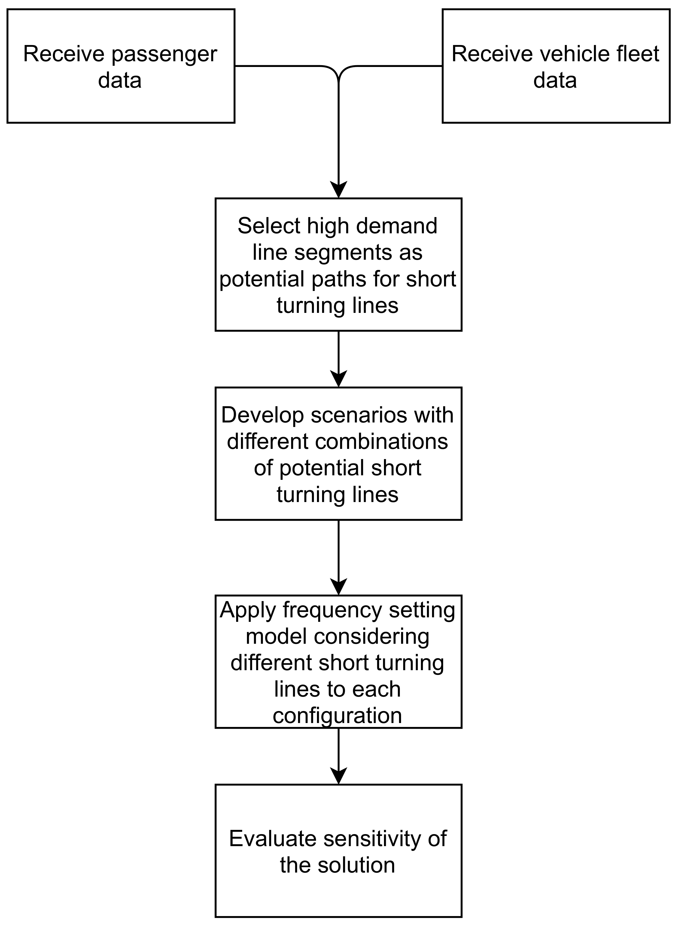
The purpose of the frequency setting model is to find optimal frequencies considering the option for short turning lines. To apply this model, data concerning passenger demand and the vehicle fleet characteristics are required. Furthermore, line segments with a high passenger demand need to be identified as potential short-turning candidates. From these alternative paths, scenarios can be constructed as the input for the frequency setting model that considers short-turning options. After the optimal frequencies and short-turning configuration are found, we examine the sensitivity of the obtained solution to the passenger demand variations with Monte Carlo simulations. These steps are schematically presented in
Figure 1.
Let us consider a public transport network consisting of lines
, where each line serves a set of stops
. Each line
l consists of a set of service patterns
. The service patterns are a product of short-turns and each pattern
serves a specific number of stops from line
l. The goal of the model is to find the optimal frequencies for each pattern in a line. The detailed nomenclature be found in
Table 2. The main assumptions in this study are:
Passenger arrivals at stops are uniformly distributed within an one-hour period; a common assumption in high-frequency services [
41,
42,
43].
The passenger demand is inelastic to changes made in the service frequencies because it is mostly affected by COVID-19.
There are no passenger transfers among the examined service lines.
At least a minimum service frequency for each line l is required to maintain a minimum level of service.
The fleet of vehicles is homogeneous.
The objective is to find the optimal allocation of buses such that (1) the revenue loss is minimized, and (2) the operational costs are minimized. The mathematical formulation of the objective function is presented in Equation (
1).
The first term in Equation (
1) represents the operational costs, i.e., the total vehicle costs. As all vehicles are assumed to be homogeneous, the total vehicle cost is the cost of a single vehicle times the number of used vehicles. The second term in the equation represents the revenue losses because of the passengers that cannot be accommodated in the considered time period due to the pandemic-imposed capacity limitations. The revenue loss per passenger consists of a minimum fare price a passenger has to pay and a fare charge for the distance the passenger would have travelled.
Since there is a limited number of vehicles available, it needs to be assured that no more vehicles are used than the total available number of vehicles:
Equation (
2) states that the total number of vehicles assigned to every service pattern
of every line
should be less than or equal to the available number of vehicles.
The service frequency of a pattern p on line l is:
bounded by the number of assigned vehicles, , divided by the corresponding round-trip travel time .
bounded by a predefined maximum and minimum frequency ().
The minimum frequency ensures a minimum service level and a maximum frequency prevents vehicle bunching that can emerge from very small time headways. The minimum and maximum allowed frequencies result in the constraints of Equation (
3) that determine the bounds of the assigned vehicles to every service pattern
.
In addition, the time headway between successive buses operating on pattern
is constrained by Equation (
4), which states that the time headway should be greater than or equal to the round-trip travel time of service pattern
p divided by the number of assigned vehicles to this pattern:
The joint frequency of all patterns on a route (e.g., section of line
) should also not exceed a maximum frequency to avoid vehicle bunching on the sections with higher passenger demand. This is described in Equation (
5):
The number of in-vehicle passengers (also known as bus load) should be computed between each stop in order to develop a model that is able to consider the pandemic-imposed capacity as a constraint. The following constraints are added to the model to address the pandemic-imposed capacity limitations:
Equation (
6) strives to maintain the in-vehicle passenger demand below the pandemic-imposed capacity for each vehicle serving a service pattern
of a line
. Equation (
7) determines the number of in-vehicle passengers after the bus departs from the first stop of the line. Equation (
8) is a recursive equation that determines the number of in-vehicle passengers for all other stops of the line. The first term on the right-hand side of the equation is the number of in-vehicle passengers during the departure from the previous stop,
, while the second term determines the number of passengers that boarded the bus at previous stops and will alight at stop
. The third term in the equation represents the number of passengers entering the bus at stop
s. It is important to note that for a service pattern
, we consider only the stops
that can be served by that pattern.
Due to the pandemic-imposed capacity, there may be no feasible solution that serves the entire passenger demand of a line
. This will result in unserved passengers. The number of unserved passengers (travelling from stop
s to
y using service pattern
p) that cannot be accommodated is represented by the variable
(Equation (
9)).
Note that if service pattern is not serving stop s or y.
The total number of passengers traveling from stop
s to
y on line
l using pattern
p is provided in Equation (
10) by aggregating the passenger demand of all user types.
In the case that some passengers cannot be accommodated due to the pandemic-imposed capacity, no priority for boarding should be given to a certain user type, as the passenger boarding process is random regarding the user type. Therefore, the passenger group that enters or is not accommodated should represent the average of the group considering the user types. That is, for any user group
, the accommodated passengers are proportional to the total demand from stop
s to
y for line
l (Equation (
11)):
Combining the objective function and the constraints results in the following mathematical program that determines the optimal service frequency of each original line and short-turning subline while considering the pandemic-imposed capacity:
The objective function in Equation (
12) is formally described in Equation (
1). Equation (
13) define the set of feasible solutions. Equations (
14)–(
17) state the domains of the corresponding variables. The mathematical model (Equations (
12)–(
17)) is a mixed-integer quadratic program (MIQP) as the model contains linear and quadratic constraints. The quadratic constraints are Equations (
4), (
7) and (
8), representing the maximum possible service frequency and in-vehicle passenger loads.
4. Case Study
4.1. Case Study Description
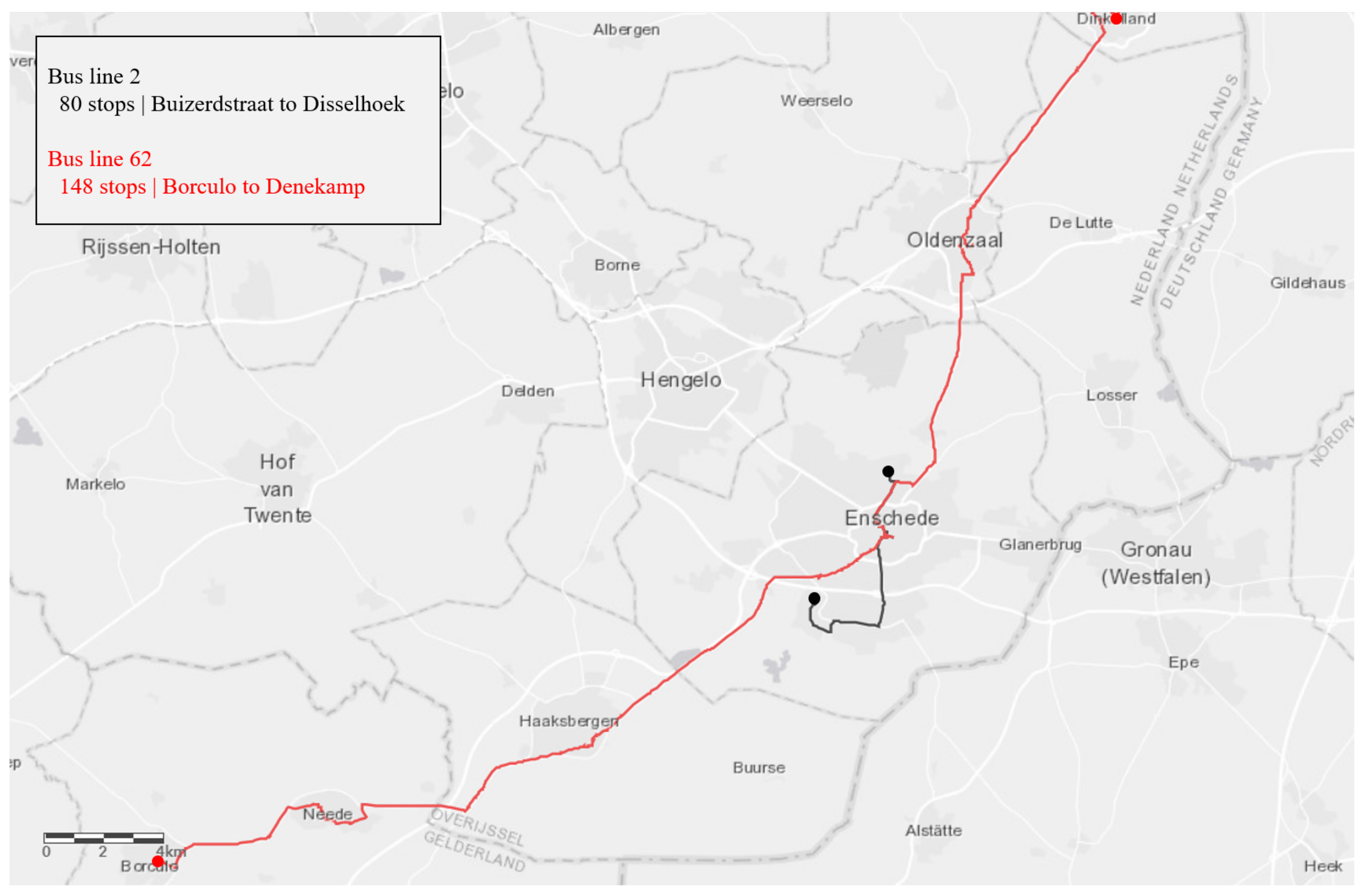
The case study involves two lines of the bus network in Twente: lines 2 and 62. The two lines were selected because they have specific line segments with abnormally high passenger demand levels that exceed the pandemic-imposed capacity, and these segments can benefit from the use of extra service frequencies. Line 2 connects the southern districts of Enschede with the northern districts. Line 62 starts from Denekamp and goes to Borculo via Enschede. Line 2 has a total of 40 stops and visits stops in one round-trip. The route is around 13 km long and the average round-trip time in the morning peak is about min. For line 62, the average round-trip time is around min. Line 62 serves in one round-trip stops. For both lines, a layover time of 10 min is included in the round-trip times.
Lines 2 and 62 are operated by Keolis Nederland, which provides the public transport service in Twente. The number of available buses that can be assigned to these lines is 16. To ensure that social distancing measures are adhered to, the pandemic-imposed capacity is set to
passengers per vehicle for lines 2 and 62. The topology of the two bus lines is presented in
Figure 2. Note that the two lines do not have passenger demand transfers, and our model assumption of no shared line corridors that result in passenger transfers is maintained.
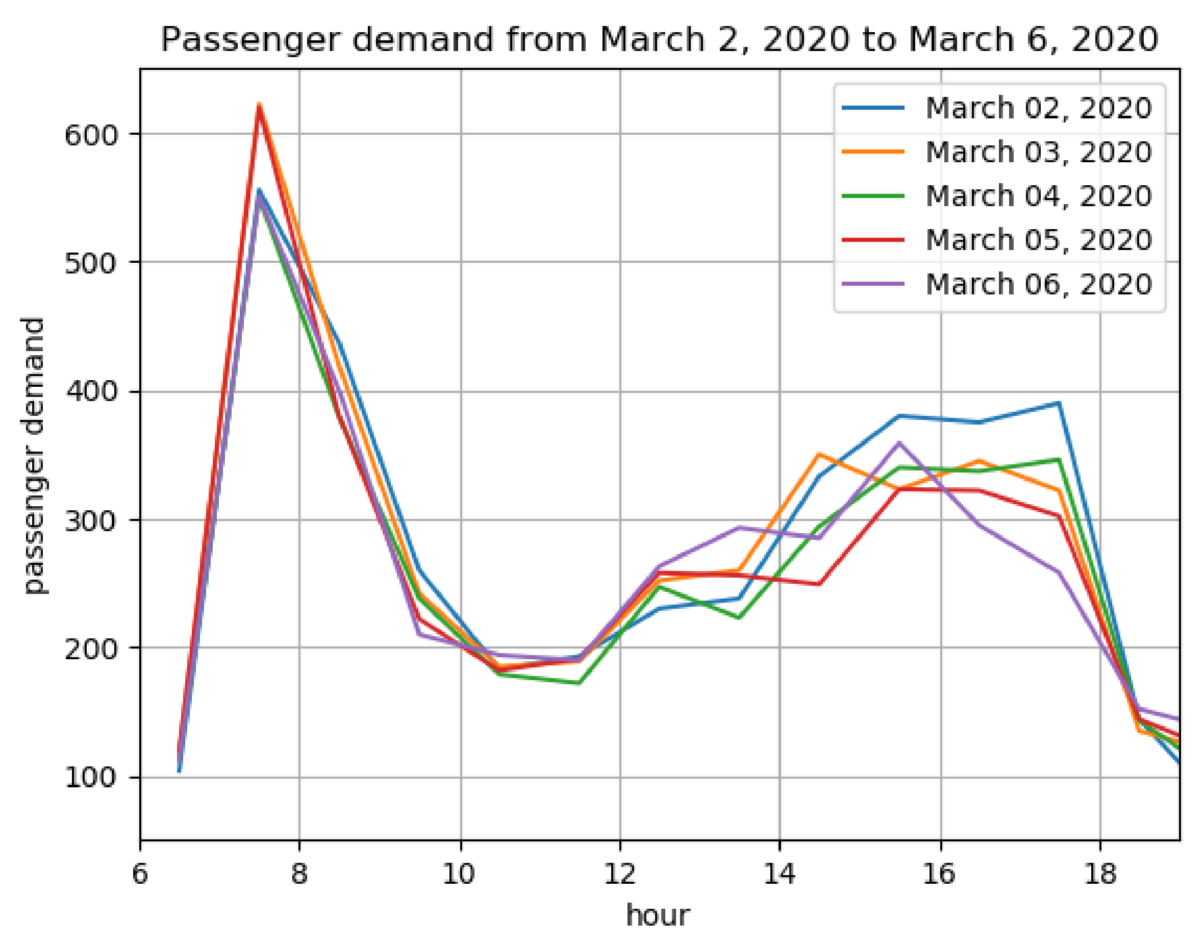
In this study, we consider a peak period in which the hourly demand exceeds the pandemic-imposed capacity.
Figure 3 and
Figure 4 show the total passenger demand for the weekdays in the first week of March 2020. For line 2, the passenger demand is at its peak in the morning between 8 and 9 a.m. for each day in that week. For line 62, this peak occurs between 7 and 8 a.m. All peak hours during the examined week exceed the pandemic-imposed capacity, and the choice was made to use the demand between 8 and 9 a.m. on Monday, 2 March 2020.
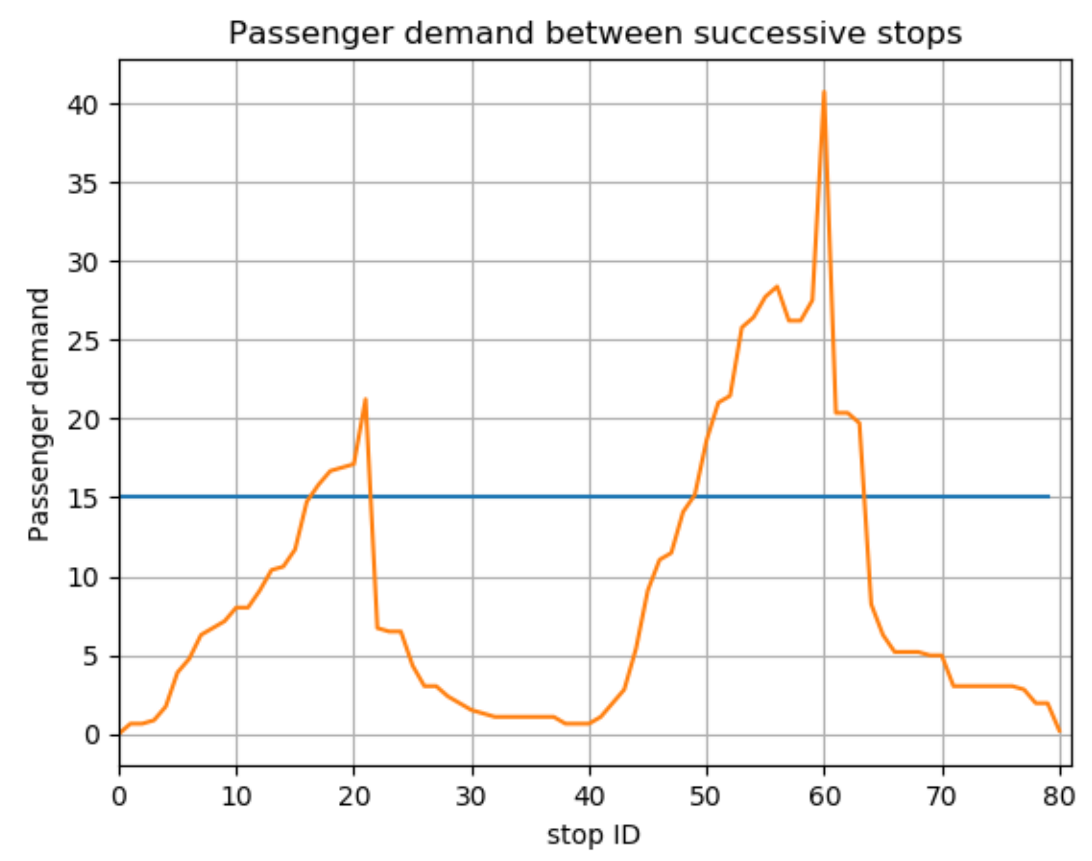
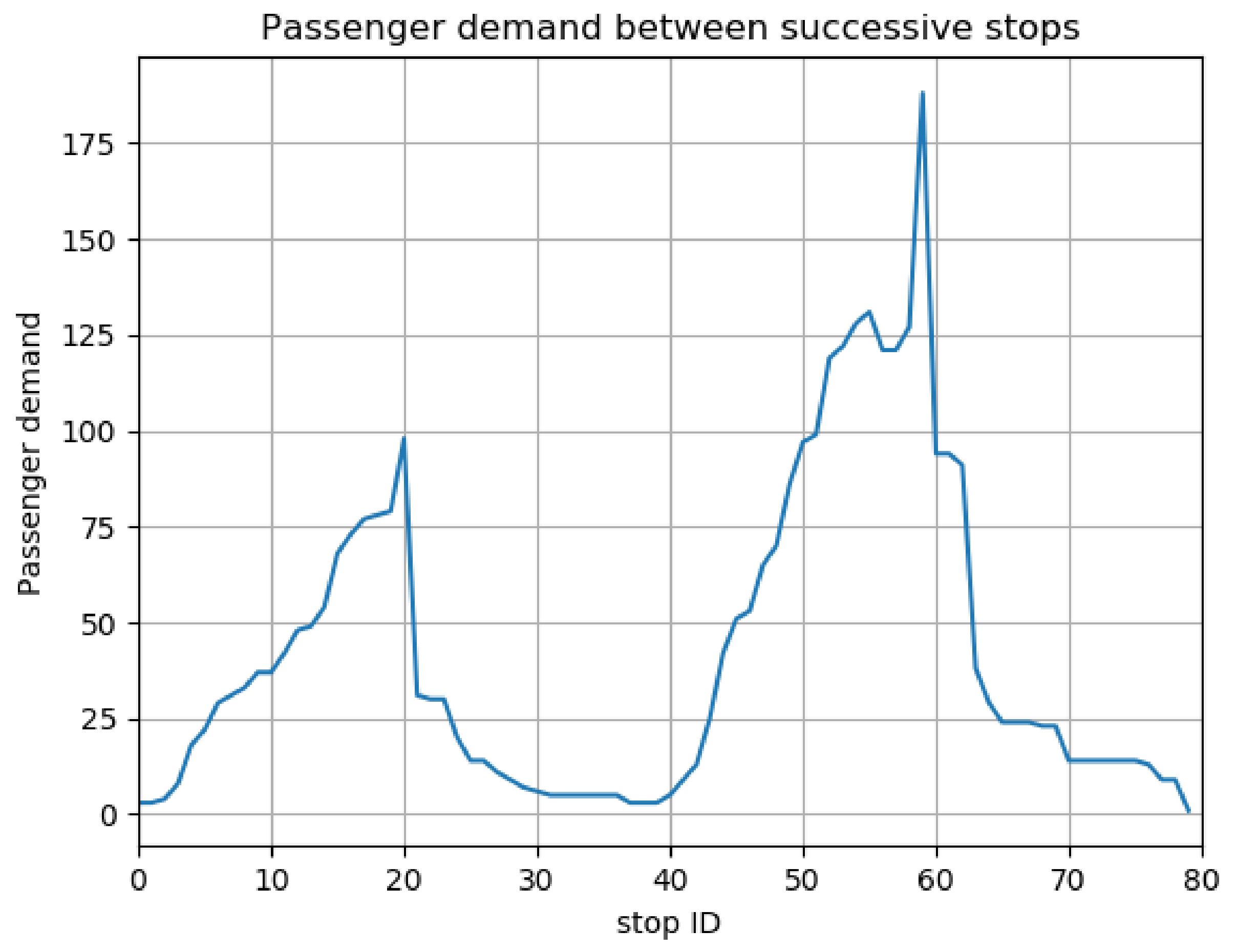
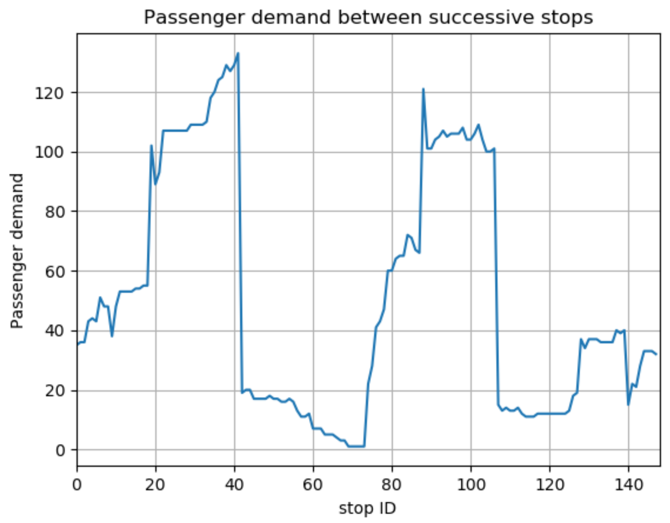
The demand between all stops for both lines 2 and 62 in the considered time period is presented in
Figure 5 and
Figure 6. In total, 757 passengers have to be served, of which 437 passengers are willing to use line 62 and 320 passengers are willing to use line 2. Both lines 2 and 62 are bi-directional and the same stop appears in both directions. The x-axis of
Figure 5 and
Figure 6 represents the stops on a line for one round-trip. For line 2, stops 1 and 80 represent Enschede Buizerdstraat. Stops 40 and 41 represent the other end of the line, which is Enschede Disselhoek. The central station of Enschede is located at stops 21 and 60.
For line 62, stops 1 and 148 represent Borculo bus station. The other end, Denekamp Onder de Linden, corresponds to stops 74 and 75. Other points of interest are the bus station of Haaksbergen (stops 20 and 129) and the central station of Enschede (stops 42 and 107).
There are a total of seven passenger types using the public transport network of Twente: adults, students, seniors, children, teenagers, business, and anonymous. The latter user group defines the passengers that do not disclose their user group information, e.g., passengers who buy paper tickets or have a smart card that is not registered to a user group. Each user type
has to pay a different minimum fare price,
, when entering a bus. In addition, each group has a different fare charge for each kilometer traveled,
. The fare prices for each user type are presented in
Table 3.
The user group ‘adults’ has the highest share in the passenger demand, with a share of 65% of the passenger demand on line 62 and 63% on line 2. The demand share of the other user groups in the passenger demand for line 2 and line 62 can also be found in
Table 3 under the columns
and
, respectively.
As previously discussed, the examined time period is the morning peak hour from 8 to 9 a.m. on Monday 2 March 2020. This hour was selected because the passenger demand is higher and this might lead to passengers that cannot be accommodated due to the pandemic-imposed capacity. As a baseline, the model of [
14] will be considered. The baseline model is a frequency setting model that sets the frequencies of public transport lines while considering the pandemic-imposed capacity limitations. The baseline model does not consider sublines (e.g., short-turning lines), and it can be used as a benchmark in order to study the effect of the service patterns that are proposed by our model. Both the benchmark model and our model that considers short-turning options and is described in Equations (
12)–(
17) are implemented in the same network using the same input values (parameters). Namely, the cost for deploying an additional bus,
W, is set to
. The maximum time headways between successive bus trips to guarantee a minimum service level are
min and
min, respectively. The minimum headway that avoids bus bunching is set to
min. The joint frequency of all service patterns on a line should also comply with the same minimum headway, as described in Equation (
5).
After applying the baseline model of [
14], including the different user types and boarding priority (Equation (
11)), to the data of 2 March 2020, the following results were obtained:
there are seven buses assigned to line 2 and nine buses assigned to line 62.
the headway of line 2 is 13 min. The headway of line 62 is 24 min.
the number of refused passenger boardings per line is 74 and 173, corresponding to 24% and 40% of the total passenger demand, respectively.
the objective function has a value of 309.94.
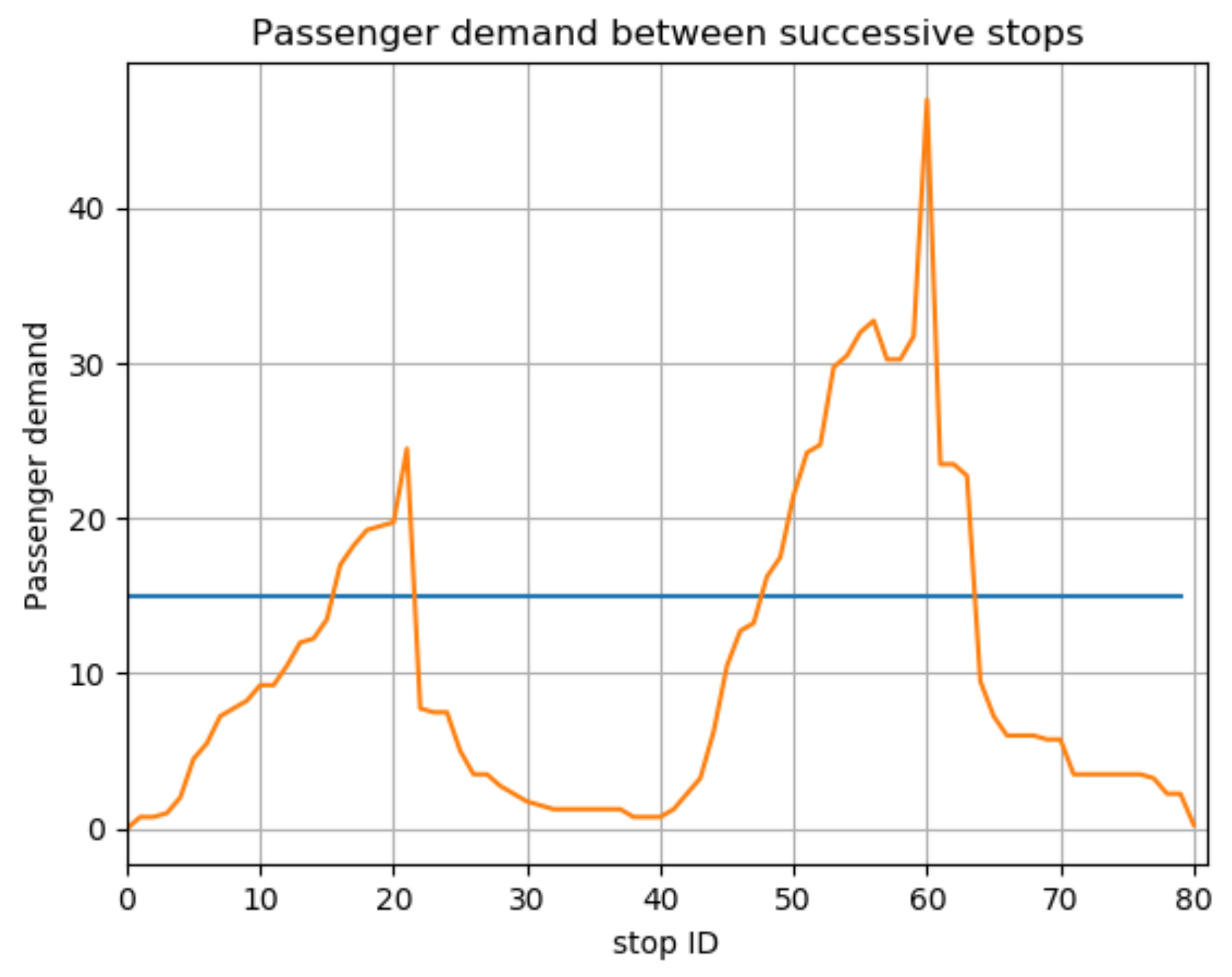
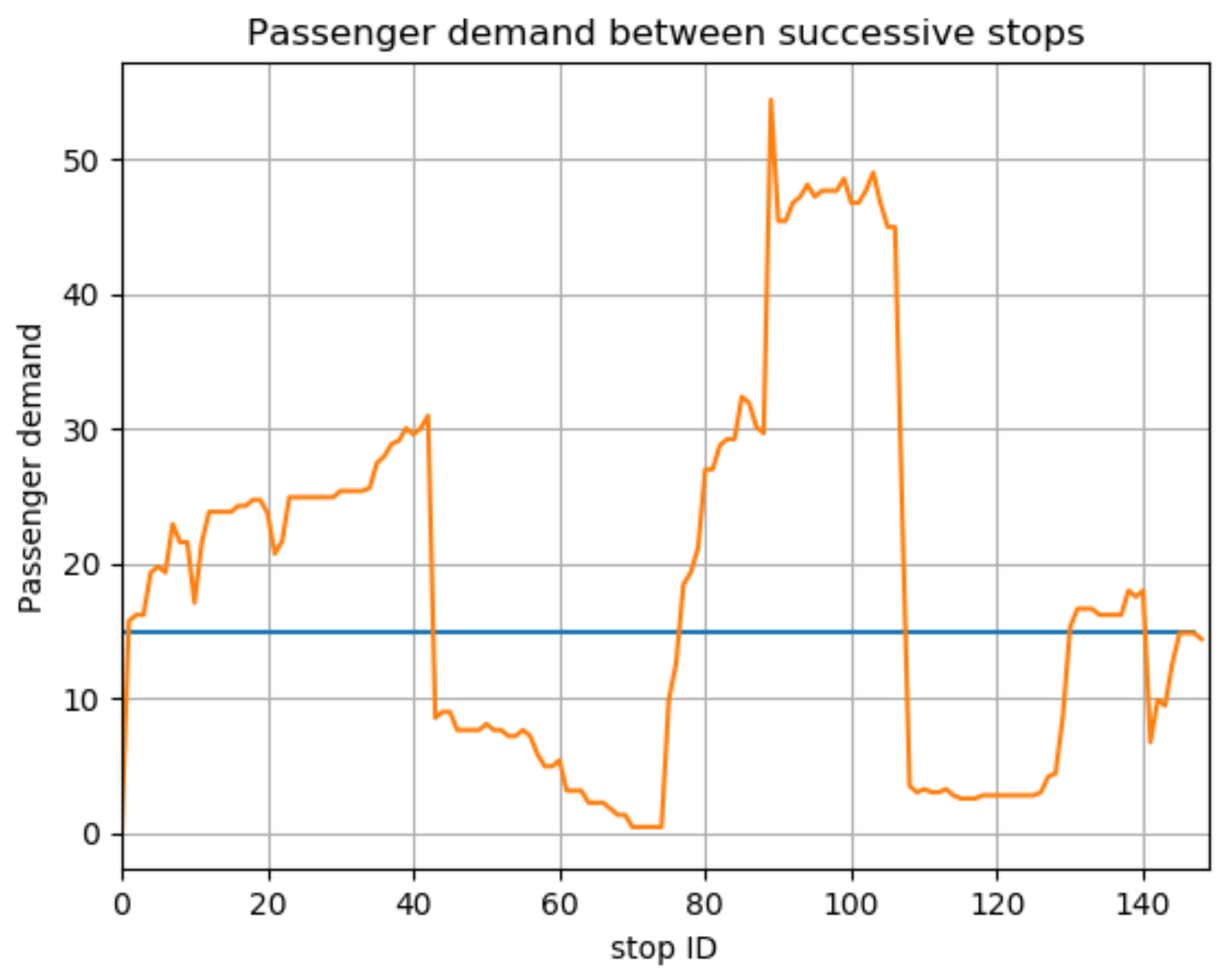
The average in-vehicle passenger demand between the stops is shown in
Figure 7 and
Figure 8. As can be seen, there are two peaks in the passenger demand for line 2. The first peak corresponds to the line segment from Enschede Hulsmaatstraat (stop 17) towards Enschede Centraal Station (stop 21). The second peak is bigger than the first and corresponds to the line segment from Enschede Disselhoek (stop 41) to Enschede Centraal Station (stop 60).
Line 62 shows a similar trend. The first capacity violation starts right after the bus station of Borculo (stop 1) and the peak starts at Haaksbergen Busstation (stop 20) and ends at the central station of Enschede (stop 42). The second peak is from Denekamp (stop 75) until the central station of Enschede (stop 107). It is clear from the aforementioned figures that short-tuning lines might provide operational benefits in terms of running costs because they can offer higher service frequencies to the high-demand line segments without having to serve the low-demand areas.
4.2. Service Pattern Selection of Short-Turning Lines
Given the passenger demand patterns in our case study, we restrict the number of short-turning lines to at most two per original line. As the service patterns on a line are most useful to line segments for which demand exceeds the supply, short-turning lines will serve the stops where the pandemic-imposed capacity is exceeded [
13].
For line 2, this means that two alternatives are considered. The first alternative is the round-trip between Enschede Buizerdstraat (stop 1) and Enschede Centraal Station. This short-turning line has a round-trip travel time of 50 min (including 10 min of layover time). The other considered short-turning line is the line between Enschede Disselhoek and Enschede Centraal Station. This short-turning line has a round-trip time of 54 min, including 10 min layover time.
For line 62, the first short-turning line that is considered is the round-trip between Haaksbergen station and Enschede Centraal Station. This service pattern has a round-trip time of 58 min, including 10 min layover time. The second short-turning line is the round-trip between Denekamp Onder de Linden and Enschede Centraal Station. This round-trip is 100 min, including 10 min layover time.
To summarize, given the passenger demand patterns in our case study, we consider the four short-turning lines tailored to the line segments with higher demand levels and the two originally planned lines. Some of these short-turning lines might be proven beneficial when assigning vehicles to them, while others might yield smaller benefits. To investigate this, we create several combinations of the potential short-turning lines. In each of these combinations, all originally planned lines are active (at least one vehicle will be assigned to them) and some of the short-turning lines are deemed active or inactive. The configurations that contain the investigated combinations are presented in
Table 4.
4.3. Frequency Settings Involving Short-Turning Lines
Our proposed mathematical model that sets the optimal frequencies of bus lines while considering short-turning sublines is programmed in Python 3.7.4 and solved using Gurobi 9.1.0. Gurobi 9.1.0 is an optimization solver that can solve mixed-integer quadratic programs to optimality. The results when solving our mathematical program expressed in Equations (
12)–(
17) are the values of the decision variables
(assigned buses) and
(inverse of the assigned frequency) for the considered bus lines
l and subline routes
r for each line
l. The optimal results for each considered configuration are presented in
Table 5. In the table, the headway variables
,
,
and
are rounded up to the nearest integer.
The results show the optimal allocation of buses and the corresponding headways for a selected configuration. In the baseline configuration, there seven assigned buses to the original line 2 and nine buses assigned to the original line 62.
Furthermore, the results show that the objective function value always increases if no short-turning line is used on line 2. If a short-turning line is used, then the best alternative in terms of the objective function value is the short-turning line serving the stops between Buizerdstraat and Enschede Centraal Station.
Considering line 62, the short-turning line between Denekamp and Enschede has the highest objective function value. This could be caused by the relatively long round-trip travel time of the short-turning line between Denekamp and Enschede.
The best objective function performance is obtained with configuration 3. This is also the only configuration that improves the objective function value compared to the baseline model that does not consider short-turnings.
Figure 9 and
Figure 10 show the average in-vehicle passenger load for lines 2 and 62 when adopting configuration 3. The effect of this configuration can be seen at the line segment between Haaksbergen and Enschede on line 62, where the peak is now significantly lower compared to
Figure 8.
Finally,
Table 6 shows the number of passengers that are not served at each configuration because of the pandemic-imposed capacity limitations. These values are obtained from the model results, as
and
represent the number of accommodated passengers and unaccommodated passengers on line
l, respectively.
Interestingly, the total number of unserved passengers in configuration 3 increases compared to the baseline model. This increase in unserved passengers can be explained by the objective function of our mathematical model, as the goal is to minimize the revenue losses that are affected by the unserved passenger kilometers and not by the total number of unserved passengers. The used number of buses is equal in the baseline model and configuration 3, but the allocation of buses exhibits a slight modification since configuration 3 assigns one more bus to line 62 and one bus less to line 2. As a result, more passengers on line 62 can be served in configuration 3, implying fewer unserved passengers on line 62 for this configuration. The improvement in the objective function value of configuration 3 compared to the baseline is an outcome of the reduced revenue loss per unserved passenger, which depends on the user type and the travel distance of unserved passengers. In more detail, as the distances between the stops of line 62 are generally higher than the distances between the stops of line 2, refusing boarding to a passenger who is willing to use line 62 results (on average) in a higher revenue loss.
4.4. Sensitivity of the Optimal Frequency Setting to Demand Variations
As passenger demand is stochastic, it should be validated that the optimal frequencies maintain an acceptable performance when passenger demand varies over time. A simulation study has been conducted to examine the sensitivity of the optimal frequency setting to demand variations.
The sensitivity analysis consists of 100 Monte Carlo simulations, each one of which considers a different passenger demand profile. For each simulation, a passenger demand matrix
B was created by generating passenger demand for each element
in the matrix
B. When generating the passenger demand for each simulation scenario, it is assumed that the sampled passenger demand is normally distributed. The mean of the normal distribution of an element
is assumed to be the passenger demand from the deterministic problem that is reported in
Figure 5 and
Figure 6. In addition, the standard deviation of the normal distribution is set as equal to 50% of the mean. Furthermore, the normal distribution is bounded by a maximum and a minimum value to prevent extreme outliers during the sampling process.
The performance of the most promising configuration of lines, sublines and corresponding frequency settings (configuration 3) is evaluated in the 100 simulation scenarios. In addition, we evaluate the performance of applying the baseline configuration in the same 100 simulation scenarios. The average objective function value and corresponding standard deviation that summarize the performances of configuration 3 and the baseline configuration are shown in
Table 7. The table shows that, when applied in 100 different demand scenarios, configuration 3 performs better than the baseline configuration.
5. Conclusions
In this study, we present a mixed-integer quadratic program that optimizes the service frequencies for original and short-turning lines considering the pandemic-imposed capacity limits and the revenue losses due to unserved passengers. The proposed model was applied on two bus lines in the public transport network of Twente, the Netherlands. The results show that our solution improves the performance of the objective function that considers the vehicle running costs and the revenue losses due to unserved passengers. This improvement is demonstrated when comparing our solution with the baseline model of [
14] that did not permit short-turnings. The benefit of our model can be explained by the reduction in vehicle running costs because we use more vehicles for targeted short-turning lines that serve high-demand line segments and the reduction in refused boardings for passengers that travel long distances.
Based on the results of our study, policymakers should consider alternative options to reduce the operational costs and the revenue losses due to unserved passengers. In the era of COVID-19, short-turning options should be considered to allocate more resources to segments of service lines with higher passenger loads. This, however, will require policymakers to employ different frequencies at different segments of the same line. Communicating this information to passengers and adapting the schedules of bus drivers to conform with the suggested modifications are important elements that should be taken into consideration in the decision making process.
The findings of this study demonstrate that introducing short-turning lines can result in a more efficient use of the existing resources and a better accommodation of the existing passenger demand. This improvement, however, has limitations given that the number of available resources is fixed. Because in-vehicle overcrowding cannot be completely avoided in the case of limited supply, additional planning measures, such as the acquisition of more vehicles that can facilitate the passenger demand at the maximum load points of the lines, should be considered (see [
6,
12]).
In terms of limitations, our model can be applied to service lines with a homogeneous fleet of vehicles. In addition, our model is only applicable to public transport networks with service lines that do not have passenger transfers. Finally, our model can be applied to case studies with passenger demand that is inelastic to service frequency changes.
In future research, the allowance of more than two short-turning lines per line could be considered. In this study, we considered two potential short-turning lines per original line because of the specific passenger demand profile of our case study. This, however, might differ from case study to case study. Our approach can also be expanded to lines that perform passenger transfers. For this, one should determine the timetables of the short-turning lines and the dispatching times of each vehicle.


