Forecasting Sea-Level Trends over the Persian Gulf from Multi-Mission Satellite Altimetry Using Machine Learning

Highlights

What are the main findings?

• Multi-mission satellite altimetry combined with machine learning accurately captures sea-level trends in the Persian Gulf.
• The proposed machine learning models outperform traditional statistical approaches in trend estimation and prediction accuracy.

What are the implications of the main findings?

• The results provide a reliable framework for monitoring sea-level rise in semi-enclosed and data-scarce marine regions.
• The approach supports coastal risk assessment and long-term planning under climate change conditions.

Abstract

One of the most significant impacts of climate change is sea-level rise, which is increasingly threatening to the coastal setting, infrastructure, and socioeconomic systems. Since a change at the sea level is spatially non-uniform and highly modulated by local oceanographic and climatic events, local or regional-scale measurements are necessary—especially in semi-enclosed basins. This paper examines the long-term variability of sea levels throughout the Persian Gulf and illustrates a strong spatial variance of the trends over the past and the future. Using three decades of satellite-derived observations, regional sea-level trends were estimated from monthly sea-level anomaly (SLA) data, which were also used to generate future projections to 2100. The analysis shows that the rate of sea-level rise along the UAE–Oman stretch is 3.88 mm year⁻¹ and that of the Strait of Hormuz is 5.23 mm year⁻¹, with a mean of 4.44 mm year⁻¹ in the basin. Statistical forecasts of sea-level change were projected by a statistical forecasting scheme with high predictive ability with the optimal configuration of an average of 0.0391 m, an RMSE of 0.0492 m, and an R² of 0.80 when independent validation was conducted. It is estimated that by 2100, the average rise of the sea level in the Persian Gulf is about 0.30–0.40 m, and the peak rise in sea level is at the Strait of Hormuz. Since these projections are based on statistical extrapolation rather than physics-based climate models, they are interpreted within the uncertainty envelope defined by IPCC AR6 scenarios. This study presents a unique, regionally resolved viewpoint on sea-level rise that is relevant to coastal risk management and adaptation planning in semi-enclosed marine basins by connecting robust statistical performance with physically interpretable regional patterns.

1. Introduction

One of the most devastating effects of climate change is sea-level rise (SLR), which is a long-term risk to coastal habitats, infrastructure, freshwater, and human settlements. An increase in sea level leads to long-term tidal flooding, irreversible submergence of land, infiltration of salt water into aquifers and agricultural soils, erosion of the coastline, and loss of coastal ecosystems like mangroves and wetlands. According to recent climate model projections, ocean thermal expansion and faster ice-sheet melt will result in a persistent rise in global sea level throughout centuries, even in moderate scenarios of reducing emission levels [1]. Consequently, coastal lowland areas will become subject to rising physical, ecological, and socioeconomic stresses in the 21st century. The reaction of the coastline towards increasing sea levels has already come into play at a global level. A report by Luijendijk et al. (2018) and Mentaschi et al. (2018) also found extensive shoreline recession of between 1 and 3 m in 1984–2015, as well as a few decimetres annually [2,3]. During the same time span, around 160 km² of land was washed away along the Atlantic and over 460 km² of land along the Indian Ocean coastlines.

On a regional level, Addo and Addo (2016) discovered that Ghana was experiencing a decline of close to 80% of its coastline between 1974 and 1996 [4]. The IPCC (2021) estimates that the majority of sandy coasts across the world will continue to recede through the 21st century, with some local accretion possibly occurring in eastern Southern Africa and western Madagascar [5]. Changes in sea level cannot be considered to be spatially homogeneous since local oceanography, evaporation, atmospheric pressure systems, vertical land movement, and circulation patterns can play a significant role in regional patterns. The Persian Gulf is a semi-enclosed basin with a high rate of evaporation, limited exchange with the open sea, and a complicated coastline geomorphology that makes it especially vulnerable to changes in the sea level. Therefore, the indicators of global averages cannot be relied on to indicate the magnitude of SLR in the Gulf, and an area-specific evaluation is needed to reflect local variability as well as risks.

Satellite radar altimetry is now the main instrument used in the measurement of long-term sea-level changes at both regional and global levels. Since 1992, sea-surface height has been continuously cross-calibrated with missions including TOPEX/Poseidon, Jason-1/2/3, ERS-2, GFO, Envisat, CryoSat-2, Sentinel-3, and Sentinel-6 MF. The Persian Gulf increased at a rate of 4.4 ± 0.4 mm/year on average between 1993 and 2022 (NOAA), which is higher than the global average [6]. Even though the contribution of the glacial isostatic adjustment (GIA) towards global sea-level rise is due to a long-term vertical motion of the land, it is usually not included in operational estimates of the sea level to ensure consistency between satellite altimetry and tide-gauge observations. The Sea Level Projection Tool of NASA incorporates IPCC AR6 projections, which allow for mapping of a region of future sea-level conditions consistently [7]. The Persian Gulf showed a rise in surface during 2020 of between 4 and 5 mm/year as compared to 1995–2014 bases. In parallel, CNES operates multi-mission altimetry, operates AVISO, and provides seasonal corrections and time filters to obtain reference global mean sea-level datasets. An average increase was seen in the Northern Hemisphere and the Indian Ocean of 3.2 mm/year and 3.45 mm/year, respectively, between 1993 and 2023, showing the effects of climatic and circulation-related variations in the basins.

Earlier works in the Persian Gulf have been dependent on the records of tide gauges to measure the rise or fall of the sea level [8,9,10,11,12,13]. Preliminary reports of the 1980s and 1990s indicated rates of 1.7 to 2.4 mm/year. Hassanzadeh et al. (2007) obtained 2.34 mm/year in eleven stations, and Alothman et al. (2010) obtained 2.42 mm/year ± 0.21 and 0.46 mm/year⁻¹ vertical land motion, respectively [10,11]. Follow-up reports revealed an increase in the rates on Mina Salman and Doha to a high of 2.8 mm/year during 1993–2013 [13]. Sea-level variability in the Gulf was measured more accurately because satellite altimetry was incorporated. Siddig et al. (2019) also discovered altimetry-based trends of 3.6 + 0.4 mm/year, which surpassed gauge-based estimates (1.6 to 3.4 mm/year) [14]. They were substantiated by Siddig et al. (2021), who employed long-term records until 2018 [15]. Abdulla and Al-Subhi (2021) found an acceleration in SLR, after 2000, and mean rates were reported to exceed 4.4 mm/year in the southern Gulf, and mean increases of 39 cm by 2100 under RCP8.5 were observed [16].

Local vulnerability reports also confirm the effects of SLR. Using a model of inundation on the Failaka Island in the future, Albanai (2020) made estimates that more than 69% of the island was likely to be submerged under three meters of rise [17]. The validation of models with ground elevation data showed a high R² (0.8019), which indicated that the model-predicted and observed elevations highly agree, and Kuwait is at a high risk of being exposed to rising sea levels. In addition to observations, predictive modelling is now required to enable long-term management of coastal risks. Classical statistical techniques like ARIMA are able to model linear trends and low-frequency variations [18,19] but fail when the forcing is nonlinear. Nonlinear dynamics and time dependencies are better addressed using machine-learning models, including Support Vector Regression, Random Forest, and LSTM [20,21,22]. Although the amount of literature on sea-level variability in the Persian Gulf is growing, there are still several valuable limitations that cannot be resolved. Most early tests had been based largely on sparse tidal gauge networks that are not uniformly spaced and are locally affected by local vertical–lateral movement and are inadequate to reflect the spatial variation of basin scales. Recent satellite altimetry-based types of studies have enhanced regional coverage, though most studies have been constrained to short-period time spans, a few missions, or basin-wide averages of trends, which fail to reveal sub-regional variations within this semi-closed and dynamically complex system. Moreover, most of the extant literature uses linear or mildly nonlinear statistical methods that do not remain faithful to non-stationary behaviour, seasonality, and transit development of long records of sea-level anomalies. Although the achievement of machine-learning techniques in global and open-ocean environments has been actively pursued, there is limited use of machine-learning techniques in the Persian Gulf, especially with long and homogenized datasets of multi-mission altimetry.

This study fills these gaps by combining three decades (1993–2023) of uniformly processed multi-mission satellite altimetry through RADS with additional statistical and machine-learning systems. The analysis involves a systematic cross-sub-region assessment of the linear trends and nonlinear temporal dynamics in the Persian Gulf by ranking methods of simple linear regression, robust fit regression, and the Neural Prophet model. Implementation of Neural Prophet, where regressors are not used outside the algorithm, allows expressing seasonal variability and the gradual evolution of trends explicitly and without hiding additional costs or resources. Taken together, these methodological and conceptual efforts give the Persian Gulf a more spatially resolved, temporally robust, and policy-relevant characterization of sea-level change that was not previously available.

2. Study Area and Data

2.1. Study Area

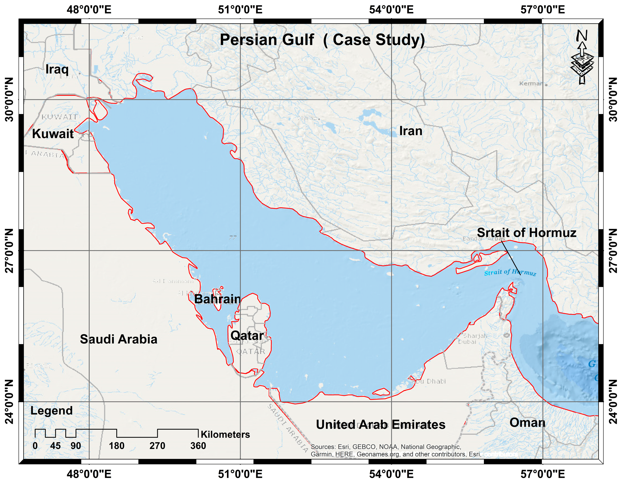
The Persian Gulf (also known as the Arabic Gulf) is an inland sea with an area of approximately 251,000 km², with a length of 816 km, and with a width ranging from 250 to 300 km, located between 24° N ≤ Latitude ≤ 30° N and 48° E ≤ Longitude ≤ 56° E, covering the entire Persian Gulf, as shown in Figure 1. The Gulf’s narrowest point is the Strait of Hormuz, which is 56 km wide. The Persian Gulf is a shallow body of water with a maximum depth of nearly 94 m and an average depth of less than 50 m. The eight nations that share the Gulf’s coasts are Iraq, Kuwait, the KSA, Bahrain, Qatar, the UAE, Oman, and Iran. The Gulf is joined to the Indian Ocean and the Sea of Oman through the Strait of Hormuz. The Persian Gulf is a semi-closed, largely shallow basin, whose limited semi-enclosed basin’s sea level with the open Indian Ocean via the Strait of Hormuz renders the gulf sea level extremely sensitive to the forces of the atmosphere, steric variations, and redistributions of mass [23,24]. Water depths that are usually less than 40 m intensify the coastal reaction to smaller alterations in sea levels, augmenting the susceptibility of the low-lying shoreline [25]. Spatial heterogeneous sea-level fluctuations are also caused by strong seasonal winds, large rates of evaporation, and background circulation of basins that cannot be well represented by sparse networks of tide gauges [26]. The Persian Gulf is specifically favourable to multi-mission satellite altimetry and regional sea-level estimations that run on data [12].

2.2. Altimeter Data

The results of multi-mission satellite altimetry were the source of the sea-level anomaly (SLA) data and were obtained through the Radar Altimeter Database System (RADS), which offers a single database of structure in any processing and harmonizing of past and present altimeter missions. In this work, RADS was taken to provide a uniform correction, bias, and quality control of all the missions before regional analysis. Measurements of the altimeter range were obtained, and then variants like atmospheric effects, geophysical effects, and instrumental effects were taken into consideration so as to eliminate non-oceanic variants before the estimation of SLA. These corrections involved ionospheric and troposphere corrections, tide corrections, sea-state corrections, and dynamic atmospheric effects. Since some of the existing RADS correction models are global, regionally related corrections have been chosen to consider the original oceanographic and bathymetric aspects of the Persian Gulf.

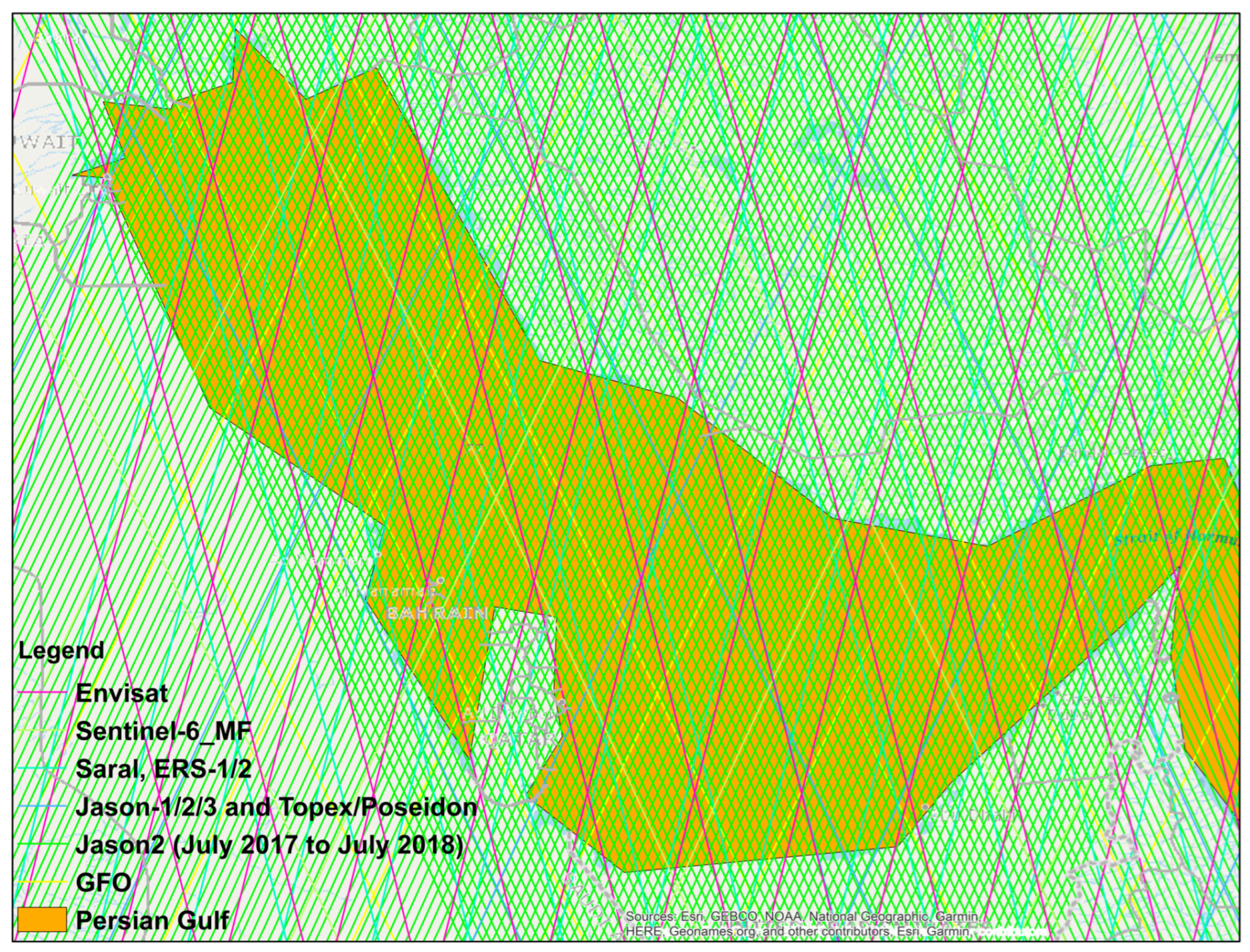
Inter-mission biases were reduced in order to make the different satellite missions consistent with dual crossover minimization analysis that allowed for the alignment of the European Space agency (ESA) class altimeters with NASA-class orbital references [27,28]. After crossover correction, SLA data were filtered and gridded with a Gaussian weighting function (2.0) to a grid with a 0.25° × 0.25° latitude–longitude grid. The use of temporal and spatial weighting was based on a nine-day cutoff window and a rectangular spatial meshwork which minimized noise but retained regional sea-level signals. Monitoring solutions of DSA were further summarized into monthly averages to facilitate long-term trend analysis of DSA and sea-level forecasts of the regions. This strategy of processing guarantees a consistency of multi-mission, strong SLA quality control and is appropriate for regional-scale sea-level assessment in a semi-enclosed basin like the Persian Gulf. Figure 2 illustrates the spatial coverage and ground tracks of multiple satellite altimetry missions (TOPEX/Poseidon, Jason-1/2/3, Envisat, ERS-1/2, SARAL, Sentinel-6 MF, and GFO) over the Persian Gulf.

For this study, a total of eleven satellite altimeter missions were utilised. These missions include TOPEX/Poseidon, Jason-1, Jason-2, Jason-3, ERS-2, Geosat Follow On (GFO), Envisat-1, Cryosat-2, SARAL, and Sentinel-3A. The total number of satellite missions utilised in this study covers 30 years. The data collected by satellite altimetry covers the time period beginning in January 1993 and ending in December 2023. Through the use of the Radar Altimeter Database System (RADS), satellite altimetry data were effectively extracted and processed. A tabular representation of the multi-mission satellite altimetry data is presented in

Table 1. Summary of all satellite altimetry data used.

Satellite	Sponsor	Period
TOPEX	NASA/Cnes	January 1993–July 2002
Jason-1	NASA/Cnes	January 2002–June 2013
Jason-2	NASA/Cnes	July 2008–October 2019
Jason-3	NASA/Cnes	January 2016–Present
ERS-1	ESA	January 1993–June 1996
ERS-2	ESA	April 1995–July 2011
Envisat	ESA	May 2002–April 2012
CryoSat-2	ESA	July 2010–Present
Saral	ESA	March 2013–December 2021
GFO	NASA/Cnes	1998–2008
Sentinel-3A	ESA	February 2016–Present

. The altimetry data that were chosen for this study are presented in detail.

3. Methods

3.1. Trend Analysis Using Simple Linear Regression and Robust Fit Regression Model Versus Neural Prophet from Machine Learning

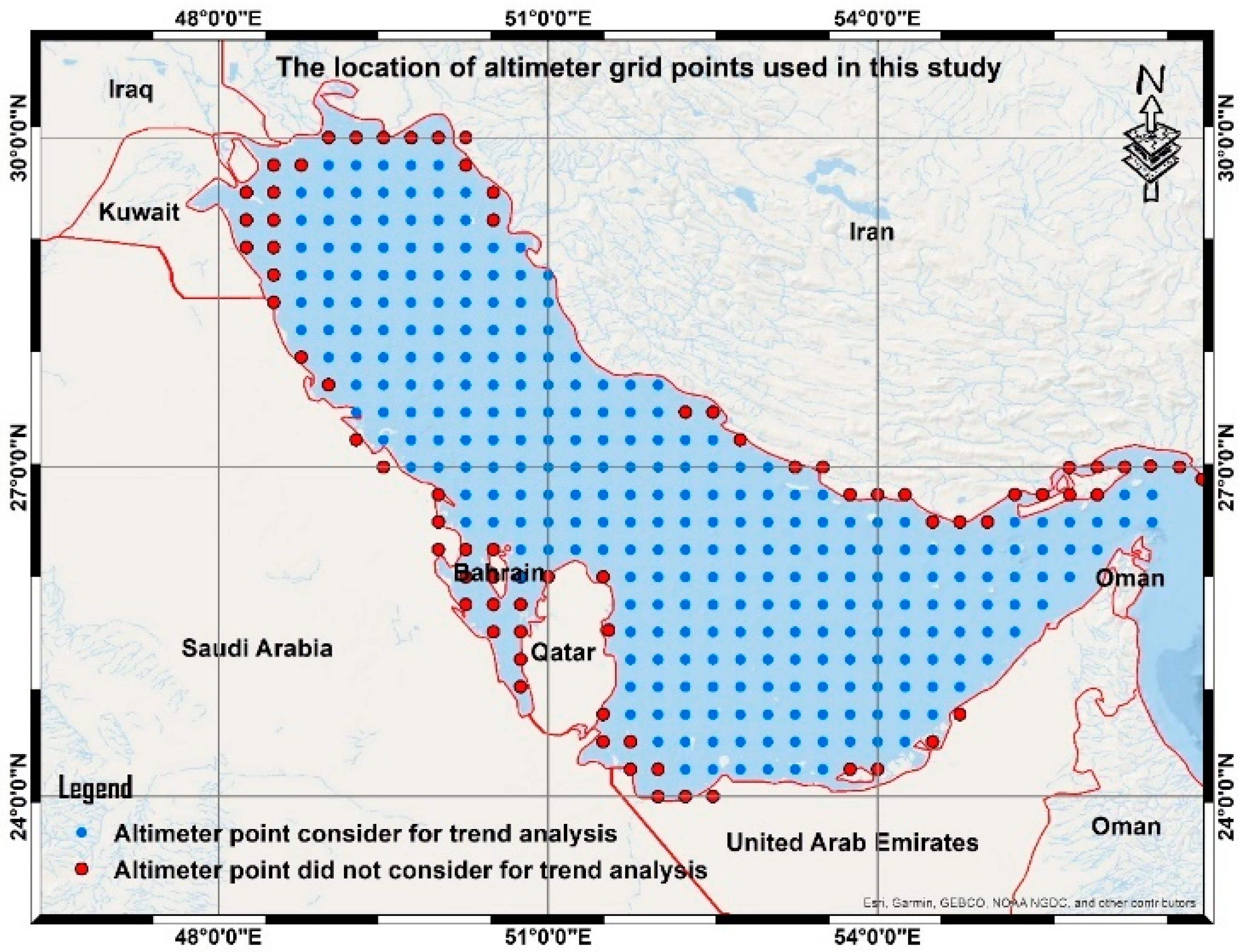
The trends at the sea level were determined based on long-term satellite altimetry records that determine the change in the height of the ocean surface over a period of time. The future sea-level change was analysed and projected using three complementary methods, which are simple linear regression, robust regression, and Neural Prophet. Linear regression has the benefit of giving an average rate of sea-level rise on a long-term average, and robust regression minimizes the effect of extreme values or short-term variability. Neural Prophet is a machine-learning-based time-series model that was employed to model nonlinear trends and seasonal variability in the data. Combining the above approaches enables transparent trend estimation as well as flexibility in forecasting and cross-comparison of outcomes. To interpret spatial and temporal variations in absolute sea level, long-term trends were analysed using satellite altimetry observations. Trend analysis was performed using the datasets obtained from 290 selected points, focusing on deep-sea and offshore areas. As explained by Anderson and Scharroo (2011), satellite altimetry-derived sea-level anomalies in coastal regions exhibit the largest residual errors [29]. Referring to Figure 3, every blue dot in the map represents an altimeter grid point used for computing absolute sea-level trends for the Persian Gulf, and all points marked in red were excluded. The equation for the simple linear regression model is given as follows [30]:

$$Y_i = {\mathit{\beta }}_0 + {\mathit{\beta }}_1{X}_i + {\mathit{\epsilon }}_i$$

(1)

where β represents monthly average sea-level changes from one period to another, ε represents the measurement standard error, and $X_i$ and $Y_i$ are the independent and dependent variables, respectively.

Based on the trend linearly plotted onto the model equation, a fitted linear trend was determined. The equation indicates whether the trend for sea-level rise has increased or decreased over the years. Subsequently, this study completed the sea-level rise forecasting process using the obtained equation. The sea-level rate for the future was obtained using this equation:

Ŷ = ƅt + c

(2)

where Ŷ is the projected value of the Y variable for t, b is the gradient value, c is the Y-intercept (estimated value of Y when t = 0), and t is the number of years that need to be projected.

In this study, robust fit regression analysis has been used to quantify the time-series of the sea-level trend. Robust fit analysis is a basic statistical technique for determining solutions and detecting outliers at the same time. An Iteratively Reweighted Least Squares (IRLSs) technique will be used to fit a linear trend to the annual sea level of each station in this robust fit strategy [31]. The weights of measurements are changed based on deviations from the trend line. After that, the trend line is refitted. The procedure is repeated until the solution is found. The adopted bi-square weight function readjusts the weights of the observations ($W_i$), whose connection with normalised residuals ($U_i$) can be written as follows [31]:

$$W_i = f\left(x\right) = \left\{\begin{array}{c}{(1 - ({U_I)}^2)}^2 \left|U_i\right| < 1\\ 0 \left|U_i\right| \ge 1\end{array}\right.$$

(3)

where $U_i = {\displaystyle \frac{r_i}{K.S.\sqrt{1 - h_i}}}$, $r_i$ is the residuals, $h_i$ is the leverage, S is the mean absolute deviation divided by a factor of 0.6745 to make it an unbiased estimator of standard deviation, and K is a tuning constant whose default value of 4.685 provides 95% asymptotic efficiency as the ordinary least squares assuming a Gaussian distribution.

Neural Prophet was used as an augmented forecasting system based on deep learning to learn temporal variations in Persian Gulf sea-level anomalies. Neural Prophet is a scaled-up version of the original phase-agnostic Prophet formulation created by Taylor and Letham (2017) [32] that introduces the concept of neural network building blocks to the framework which enables the model to capture nonlinear trends and dynamic seasonal structures [33]. The model breaks down the time-series into trends, seasonal factors, and noise according to an additive representation:

$${ y}_t = g\left(t\right) + s\left(t\right) + h\left(t\right) + \epsilon \left(t\right)$$

(4)

where g(t) describes a piecewise-linear trend (or “growth term”), s(t) describes the various seasonal patterns, h(t) captures the holiday effects, and ε(t) is a white noise error term [32]. In this study, monthly sea-level anomaly time-series based on satellite altimetry do not have any significant holiday-type events. Thus, in any of our experiments, we did not specify a holiday calendar and essentially set h(t) = 0. Only trend and seasonality components were used in the Prophet implementation, and the holiday component was turned off. Although Neural Prophet has high predictive accuracy, it has its own limitations, which should not be overlooked. Prophet is a machine-learned time-series prediction model that learns the tendencies and seasonality only based on past observations and makes no direct attempt to model physical climatic forcing processes, including ocean thermal expansion, glacier and ice-sheet mass loss, or atmospheric–ocean interactions [33,34]. Consequently, its projections are the statistical extrapolation of past patterns that may not entirely reflect non-stationary behaviour related to accelerating climate change [5].

Anomalies of monthly sea-level records calculated through multi-mission satellite altimetry, from January 1993 to December 2023, were extracted from the Radar Altimeter Database System (RADS) and used to train the model. To maintain the spatial heterogeneity and not smooth the local dynamics into a global solution, separate Neural Prophet models were built in each sub-region of the Persian Gulf coastline. The piecewise linear growth function was used to depict non-stationary sea-level development to reflect gradual acceleration and local trend divergence. The monthly temporal resolution directly supplied seasonal cycles and allowed the model to mimic intra-annual and annual sea-level changes in semi-enclosed basins like the Persian Gulf [35,36]. The inherent predictability of altimetry observations was assessed without external regressors. The training of the models was performed by stochastic gradient optimisation with automatic backpropagation using the computational graph engine of PyTorch [33]. At every iteration, model parameters such as change points, trend coefficients, and seasonal weights were optimised by minimising the loss of the mean squared error (MSE) between observed and predicted values of SLAs. The optimisation was performed in several iterative epochs until convergence. Fitting was conducted with the fit() routine, which reads time value pairs in the form of timestamp-indexed sequences. The Mean Absolute Error (MAE), Mean Squared Error (MSE), Root Mean Squared Error (RMSE), Mean Absolute Percentage Error (MAPE), and coefficient of determination (R²) were used as the model validation methods, as performed in other climate and environmental forecasting research [37,38]. The indicators of performance were reported on a regional basis, which directly compared simple linear regression and robust fit regression. Neural Prophet was always found to have higher predictive power, especially in areas where nonlinear trends and strong seasonality are observed, which validates the recent forecasting research finding that identifies Neural Prophet as being effective in non-stationary contexts [36].

3.2. Sea-Level Quantification and Projection

Historical observations of sea-level and climatic factors that contribute to sea-level changes are utilised in modelling and analysis approaches. During the last few years, simple linear regression as well as some robust linear techniques have been popularly employed to examine and sometimes forecast sea-level variations at different spatial scopes [12,14,39]. Moreover, it has recently been applied for prediction using various machine-learning techniques with Neural Prophet. Since this is seldom used in sea-level forecasting, the results of this study indicate that it can be used effectively. For example, water temperature and turbidity changes of a seasonal nature caused by climate change were forecast in the Ganga River using Neural Prophet, which produced better results than the Seasonal ARIMA model [37].

Neural Prophet has been used in recent times in the forecasting of temperature data [35,36,38]. It proved to be efficient with regard to computational time in comparison to other techniques and was the best model to deal with multicomponent seasonality, interannual trends, temporal variations, long-term seasonal component forecasting, and anomaly detection. There was another instance that experimented with the use of Neural Prophet in sea-level forecasting and compared this to that of simple and robust linear regression models.

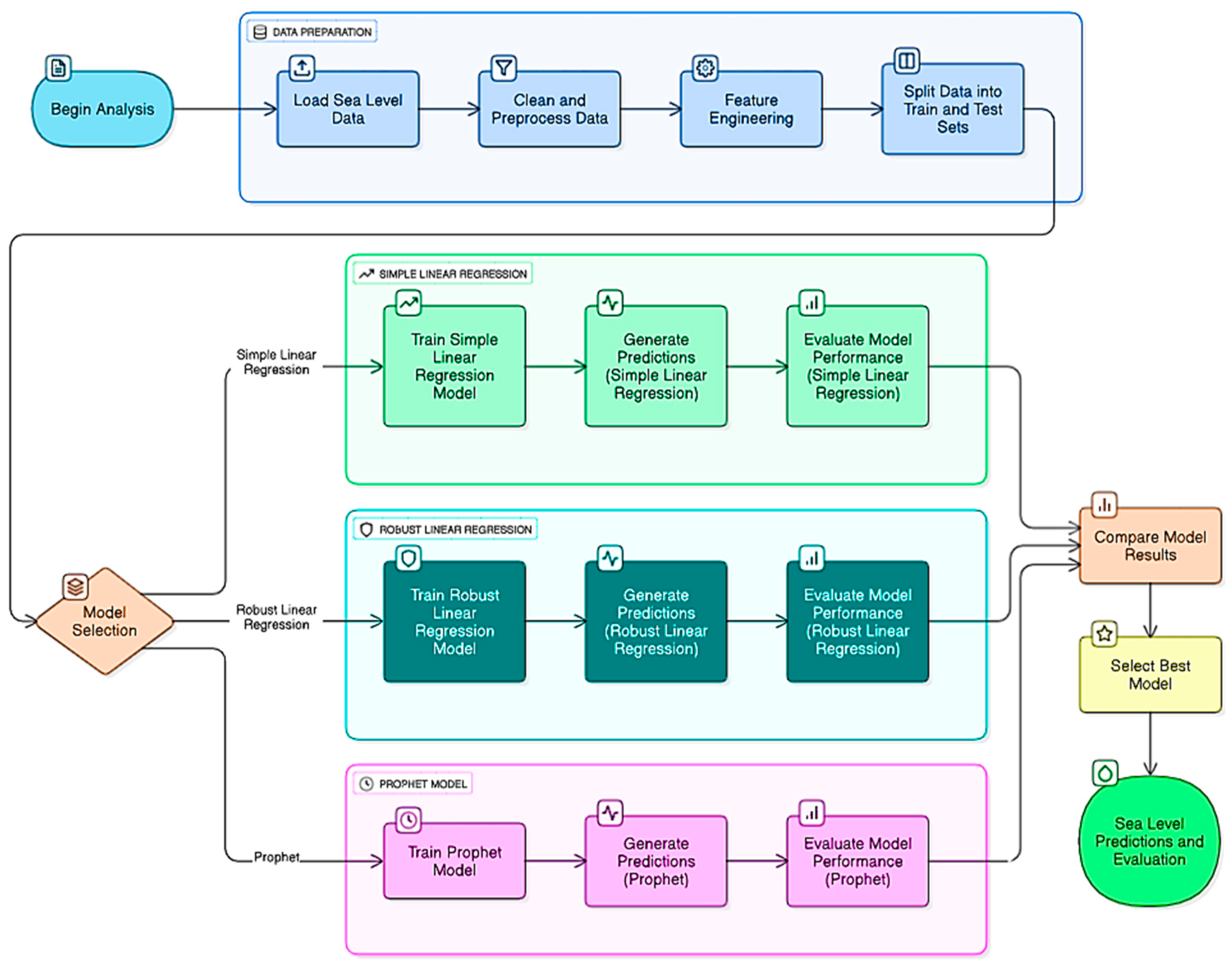
Three analysis methods were used in this study: simple linear regression, robust fit regression, and Neural Prophet. These analyses were applied to identify trends in annual mean sea-level datasets over the Persian Gulf. The modelling methodology for sea-level prediction is shown in Figure 4. The robust model, which is more resistant to outliers than simple linear regression, estimates the linear trend more reliably, but it presupposes a linear relationship and does not capture complicated nonlinear patterns or seasonality. Instead, Facebook built Neural Prophet to forecast time-series data. It handles time-series data with severe seasonal effects and historical data with missing values or outliers. It breaks time data into trends, seasonality, and holidays. Neural Prophet is developed for seasonal time-series data, is robust to missing data and outliers, and can incorporate known future events (holidays). Neural Prophet can be harder to understand and tune than linear models. The decomposition presupposes additive or multiplicative components, which may not accurately represent the process. Time-series data quality and properties determine its performance. The time-series split was used to divide the entire satellite altimetry time-series (January 1993–December 2023) in a manner that enables the time integrity of the time-series, as shown in Figure 4. The training data (January 1993–December 2016) was only utilised in the development of the model and estimation of the parameters. In the case of the linear regression model, this entailed the estimation of the slope and the intercept of the trend line. In the case of robust regression, the Iteratively Reweighted Least Squares (IRLSs) algorithm was used on the training set to down-weight the outliers and achieve a stable linear trend. Neural Prophet was optimised with the help of stochastic gradient descent, and the regression models were fitted with the least-squares and robust reweighted methods, respectively. None of the stages of model calibration used the testing data (January 2017–December 2023). Rather, they were only to be used in an independent performance assessment. Observed sea-level anomalies and model predictions based on the trained models were compared to compute error measures.

Figure 4 presents an entire process of sea-level prediction and model verification. The first stage involves data preparation, where data at the sea level are loaded, cleaned, and preprocessed, and the data with the relevant features are engineered, and then, the dataset is divided into a training and a testing set. This is followed by the application of three modelling methods simultaneously which are simple linear regression, robust linear regression, and the Prophet forecasting model. All models have a similar series of actions, which include training the model, future predictions of sea level, and the statistical measures of the model. A system comparison of the results of all three models is then carried out to evaluate their comparative accuracy and strength. On this comparison, the most performing model is chosen. Lastly, the selected model is utilized in sea-level prediction and evaluation that aids in credible long-term sea-level increment assessments.

4. Results and Discussion

4.1. Sea-Level Rate Analysis Using Simple Linear Regression and Robust Fit

A linear trend of absolute sea level has been quantified using both simple linear regression and robust fit regression to project sea-level rise in the Persian Gulf. In this section, the time-series of monthly sea-level anomalies derived from satellite altimetry data are plotted, with the objective of quantifying the rate of sea-level change using the robust fit regression technique across the Persian Gulf countries. The analysis process, using simple linear regression and robust fit regression, divided the Persian Gulf into six main regions: the Hormuz Straits, Iran coast, Iraq and Kuwait coasts, Kingdom of Saudi Arabia coasts, Qatar and Bahrain coasts, and UAE and Oman coasts. The eastern side of the Persian Gulf includes the Iranian coast, while the northern part includes Iraq and part of the Iranian coast as well. The eastern side includes several coastal countries: Kuwait, Saudi Arabia, Qatar, and Bahrain. The southern part includes the UAE and Oman, as shown in Figure 5. Therefore, the point of sea-level anomaly extraction in this study is more focused on the offshore and deep ocean areas by considering them to be within the Persian Gulf, which is the research area of interest.

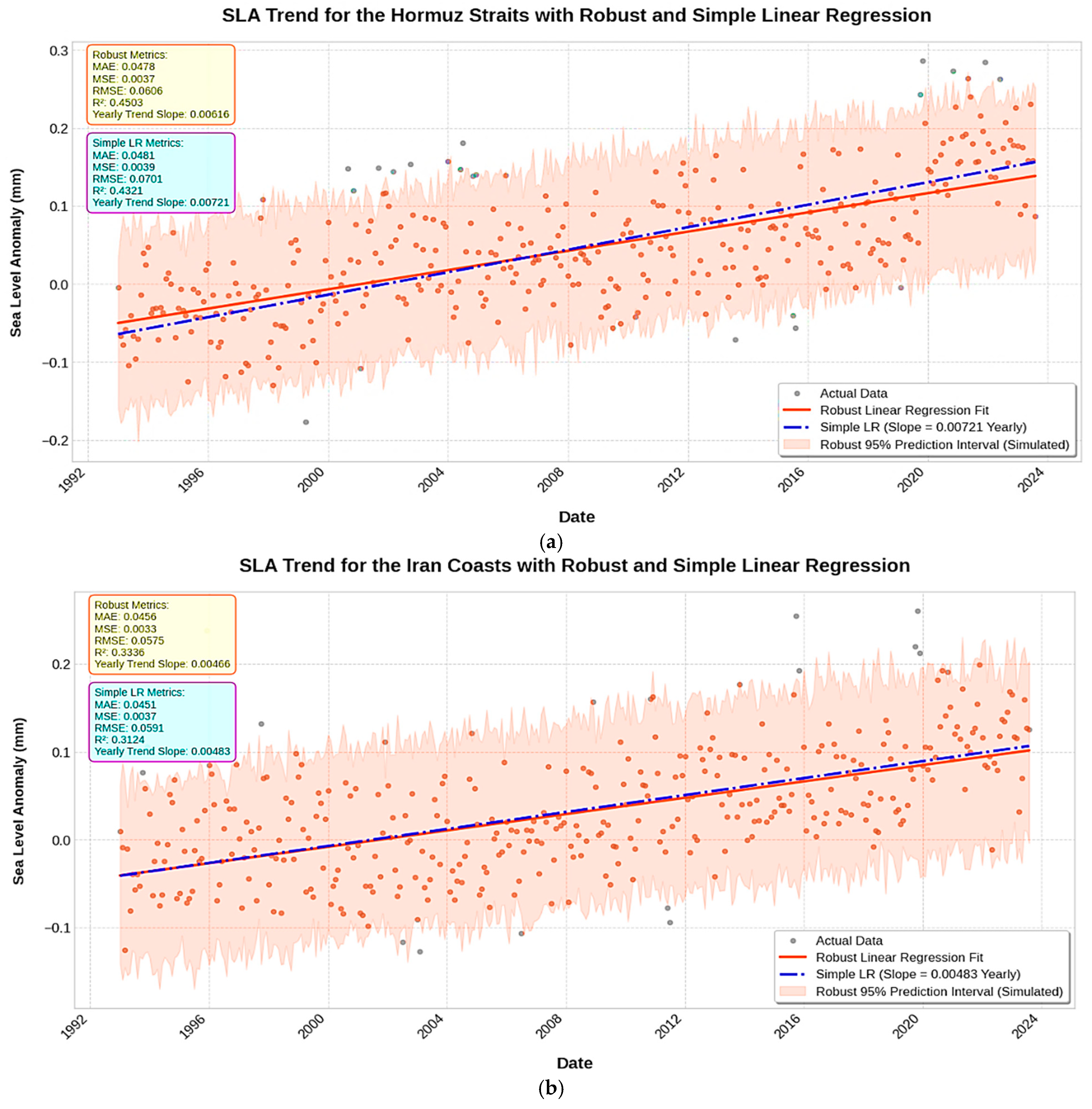
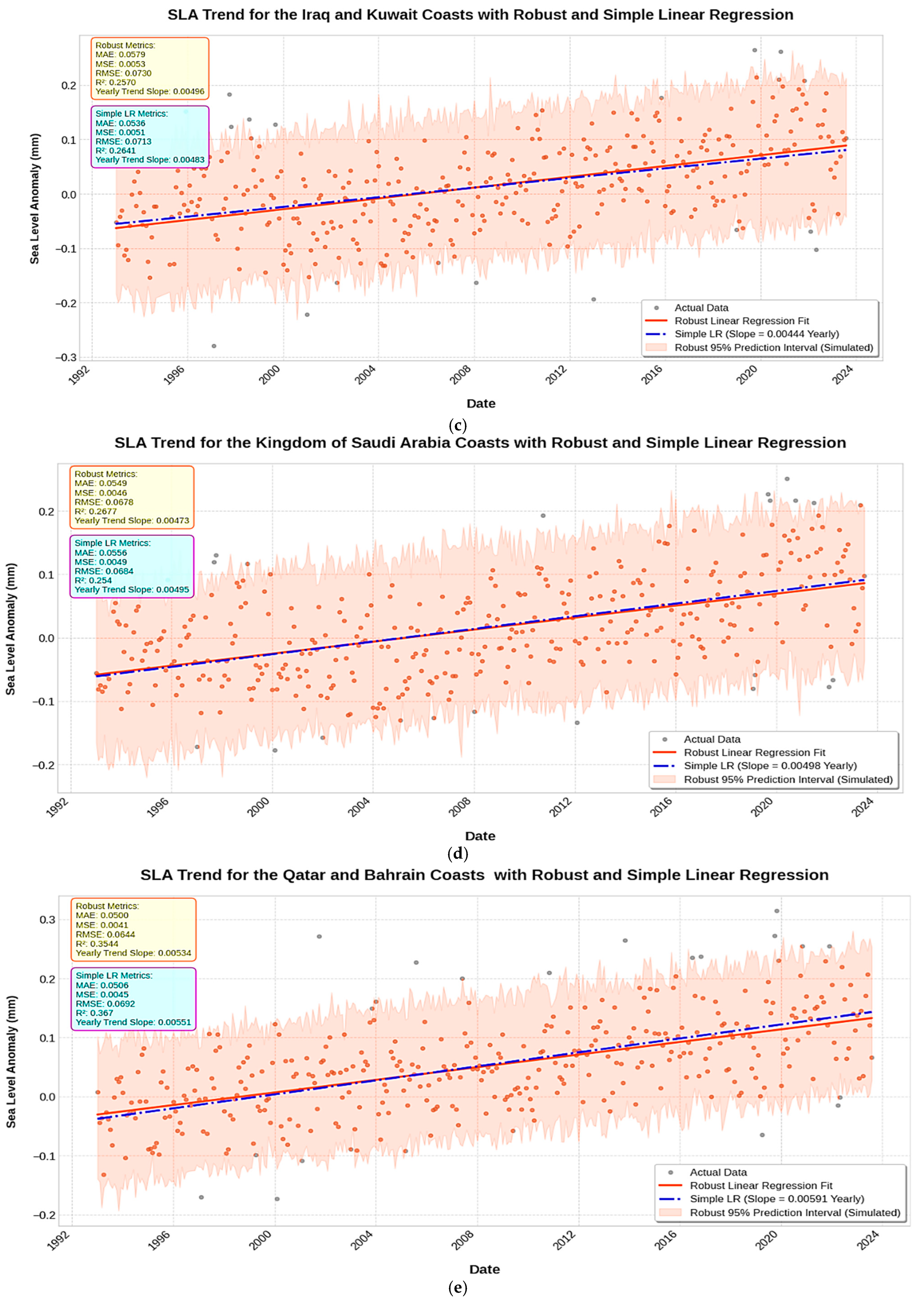
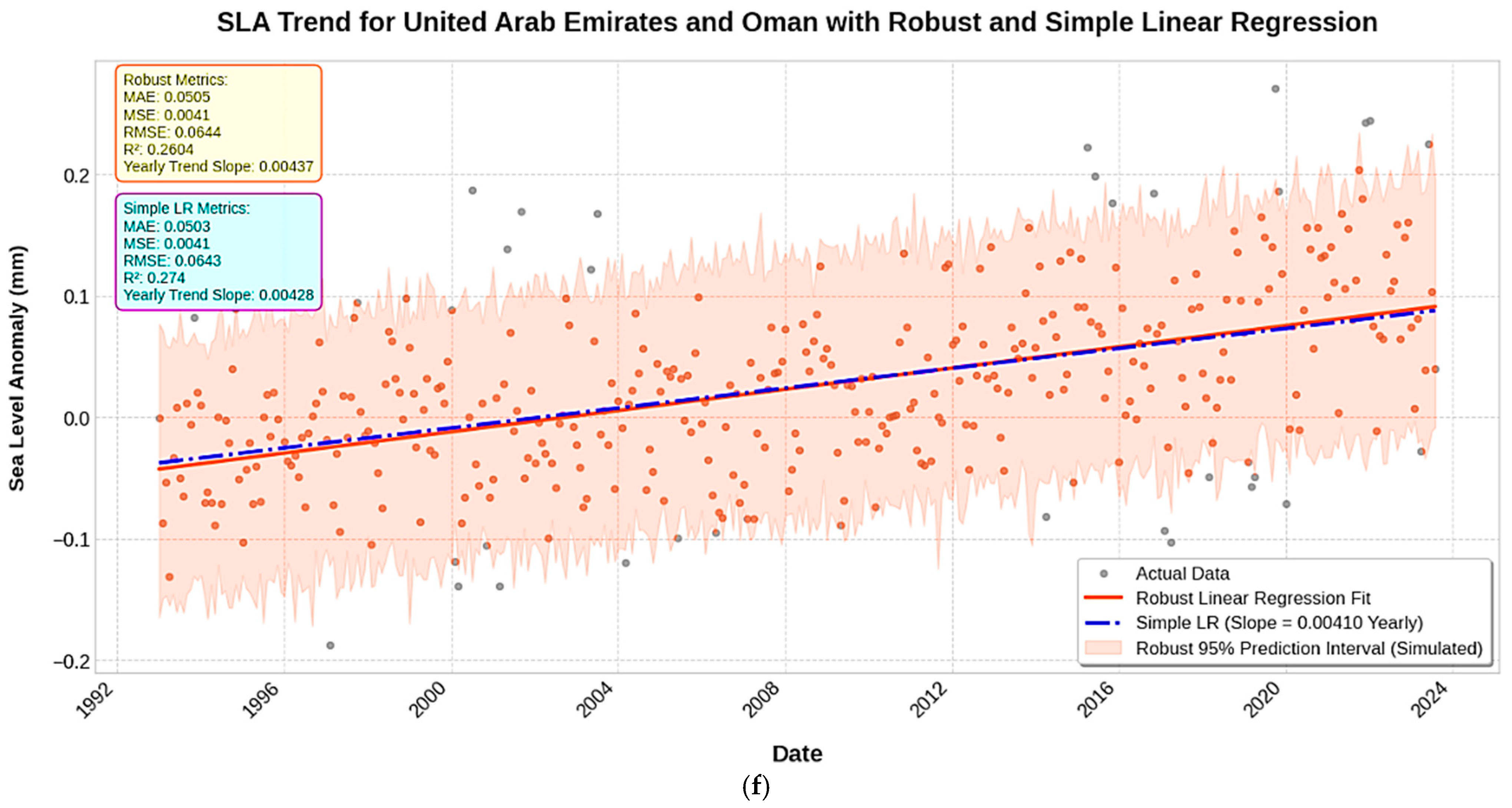
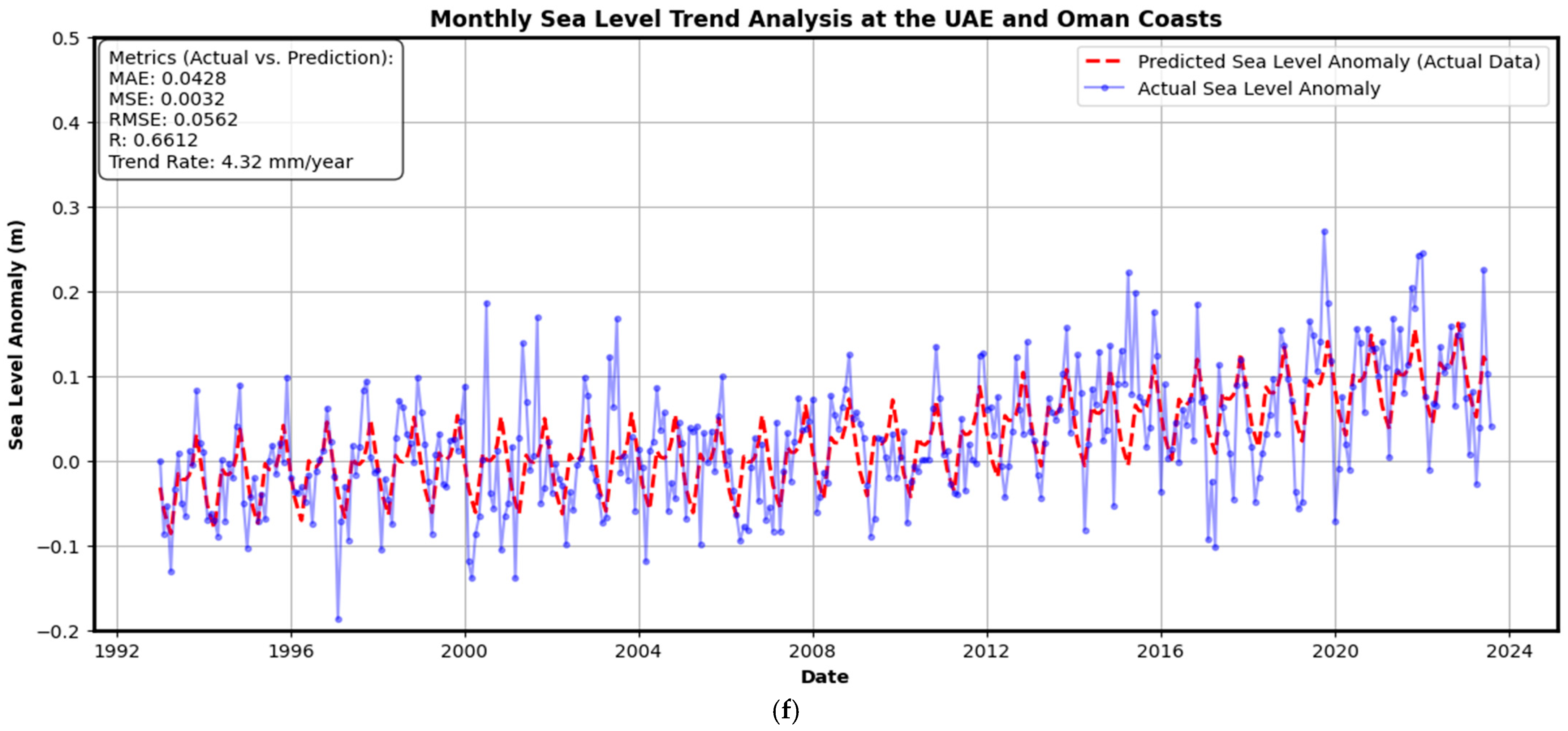
Figure 5 shows how monthly sea-level anomalies (SLAs) based on satellite altimetry have evolved long term across 6 representative coastal sectors around the Persian Gulf and has been assessed using simple linear regression (blue line) and robust linear regression (red line). In the Strait of Hormuz (Figure 5a), a significant and stable positive SLA pattern is found, which is due to the open-ocean effects and exchange with the Gulf of Oman, and the strong regression is a more refined estimate, as it provides the impact of extreme values. Figure 6b shows that the sea level is steadily rising with moderate variance along the Iranian coasts and that the two-regression models show close consistency, which means that there is consistent long-term signal of an increase. The short-term variations and broader uncertainty bands of the Iraq and Kuwait coasts (Figure 5c) are typical of shallow and low-lying waters on the north of the Gulf; however, both regression methods reveal a statistically significant upward trend. In the case of the Kingdom of Saudi Arabia coasts (Figure 5d), the variability of SLAs is relatively moderate, and the almost parallel regression lines indicate a small effect of outlier and a linear increase in sea level. A strong and consistent upward trend is exhibited in the Qatar and Bahrain region (Figure 5e) with a high concentration of the observations around the fitted lines, showing that there is a high level of consistency in the observed sea-level rise. Lastly, the coasts of the United Arab Emirates and Oman (Figure 5f) are characterized by observable interannual variability because these regions are more open to the influence of open-ocean processes, but the long-term signal is positive and strong in both regression methods. On the whole, Figure 5a,f are consistent in showing a basin-wide sea-level rise signal, and the high quality of the regression strategy is specifically useful in minimizing the impact of outliers and maximizing the trend accuracy in the altimetry analysis of the coastlines.

Table 2. Summary of statistical metrics between actual and predicted sea level using robust regression within the period of 1993 to 2023.

Region	MAE (m)	MSE (m2)	RMSE (m)	R2 Value	Sea-Level Rate (mm/Year)
Hormuz Straits	0.0475	0.003	0.063	0.45	5.54 ± 0.35
Iran coasts	0.0641	0.003	0.0035	0.25	4.30 ± 0.31
Iraq and Kuwait coasts	0.0581	0.005	0.071	0.27	4.75 ± 0.4
Kingdom of Saudi Arabia coasts	0.0551	0.004	0.0636	0.26	4.61 ± 0.39
Qatar and Bahrain coasts	0.0527	0.004	0.0632	0.38	4.41 ± 0.29
UAE and Oman coasts	0.0502	0.004	0.0662	0.28	4.12 ± 0.3
Average	0.0546	0.004	0.055	0.33	4.62 ± 0.34

and

Table 3. A summary of statistical indices of the actual and predicted sea level using simple linear regression for the period of 1993–2023.

Region	MAE (m)	MSE (m2)	RMSE (m)	R2 Value	Sea-Level Rate (mm/Year)
Hormuz Straits	0.0491	0.004	0.071	0.43	6.68
Iran coasts	0.0471	0.004	0.058	0.32	4.62
Iraq and Kuwait coasts	0.0542	0.005	0.07	0.29	4.63
Kingdom of Saudi Arabia coasts	0.0568	0.005	0.0725	0.24	4.86
Qatar and Bahrain coasts	0.0524	0.004	0.0695	0.34	4.59
UAE and Oman coasts	0.0501	0.004	0.0601	0.29	4.01
Average	0.052	0.004	0.066	0.32	4.90

provide a synthesis of the quantitative results of sea-level trend analysis across the Persian Gulf as a robust regression model and simple linear regression of the 1993–2023 record of satellite altimetry observations and demonstrates a sustained basin-wide increase in mean sea level. In all sub-regions, the two models show relatively minor prediction errors, where the values of MAE and RMSE are usually in the range of 0.05–0.06 m and 0.06–0.07 m, respectively, affirming a strong agreement between observed and modelled sea-level anomalies. The coefficients of determination (R²) lie between about 0.24 and 0.45, which is the moderate level of explanatory power, and demonstrates a strong spatial heterogeneity of sea-level behaviour caused by regional oceanographic and atmospheric processes. Three estimates of the sea-level rise are in the range of 4.0 to 6.7 mm/year, all of which the Hormuz Straits have had the highest rates (approximately 6.5–6.7 mm/year) and better model performance. The other coastal sectors have lower R² values, indicating more short run variability and local effects which cannot be modelled completely by the linear trend models. The strong regression estimates give slightly more conservative estimates of the trend with a regional average of about 4.6 mm/year, and simple linear regression estimates a slightly higher average of about 4.9 mm/year across the basin. Generally, the quantitative findings in both tables are consistent in confirming an accelerated sea-level rise of about 45 mm/year throughout the Persian Gulf and also indicate marked regional differences in the intensity of the trend and model dependability that is crucial in the interpretation of coastal exposure and flood-risk measurements.

The Persian Gulf region has shown an overall rise in sea level, as presented in Table 3, which reports positive trends across all selected sub-areas of the Gulf based on simple linear regression analysis. The lowest rate of sea level rise was recorded on the coasts of Oman and the UAE, at 4.01 mm/year, while the Strait of Hormuz stood highest, with 6.68 mm/year. In a fusion of all measurements of rates along the Persian Gulf shoreline, the robust fit regression method gave an average and consistent sea level trend of 4.90 mm/year.

4.2. Sea-Level Rate Analysis Using Prophet’s Model

A strong and flexible time-series forecasting framework is offered by Neural Prophet, which provides handling seasonality, trends, and external regressors for analysing and predicting time-series data. In this study, machine learning was applied to analyse sea-level anomalies through time for the forecasting of its future values. The training of Neural Prophet of machine learning was carried out using such data, with Neural Prophet being a more improved version of Facebook’s Prophet Methodology. Dictated by a functioning hybrid framework model based on PyTorch (https://pytorch.org/), it provides full automation whilst letting users adjust and tune datasets per their liking [33]. This Python (https://www.python.org/) script trains a time-series forecasting model using Neural Prophet on the data contained in the DataFrame (df). The Prophet object for training the model is initialised first by assigning the variable name ‘m’. The fit() method then trains the model, taking the DataFrame (df) containing the time-series data as its main argument. Another optional argument, freq, indicates data frequency—in this case, set to “M” for monthly intervals.

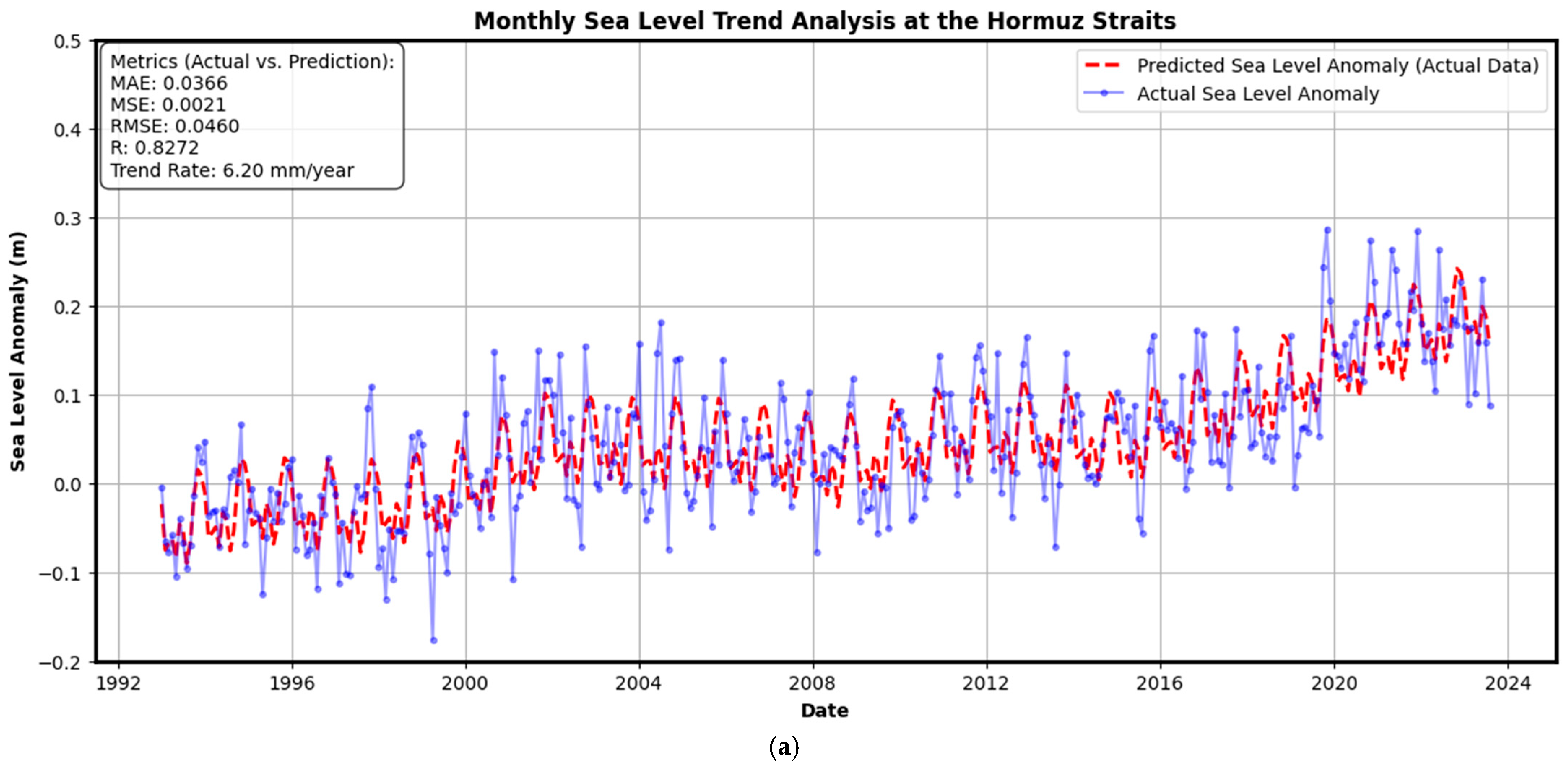
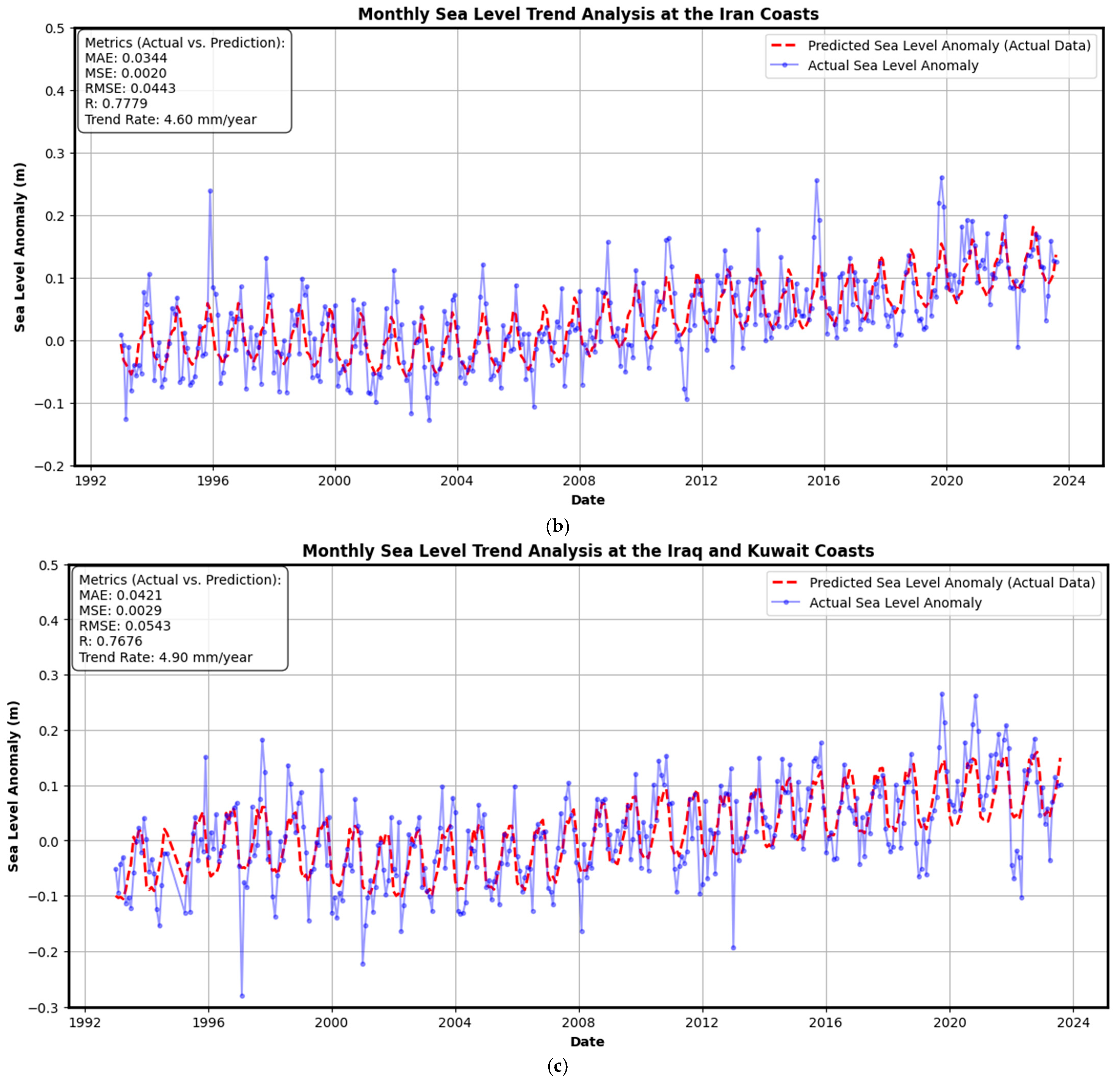
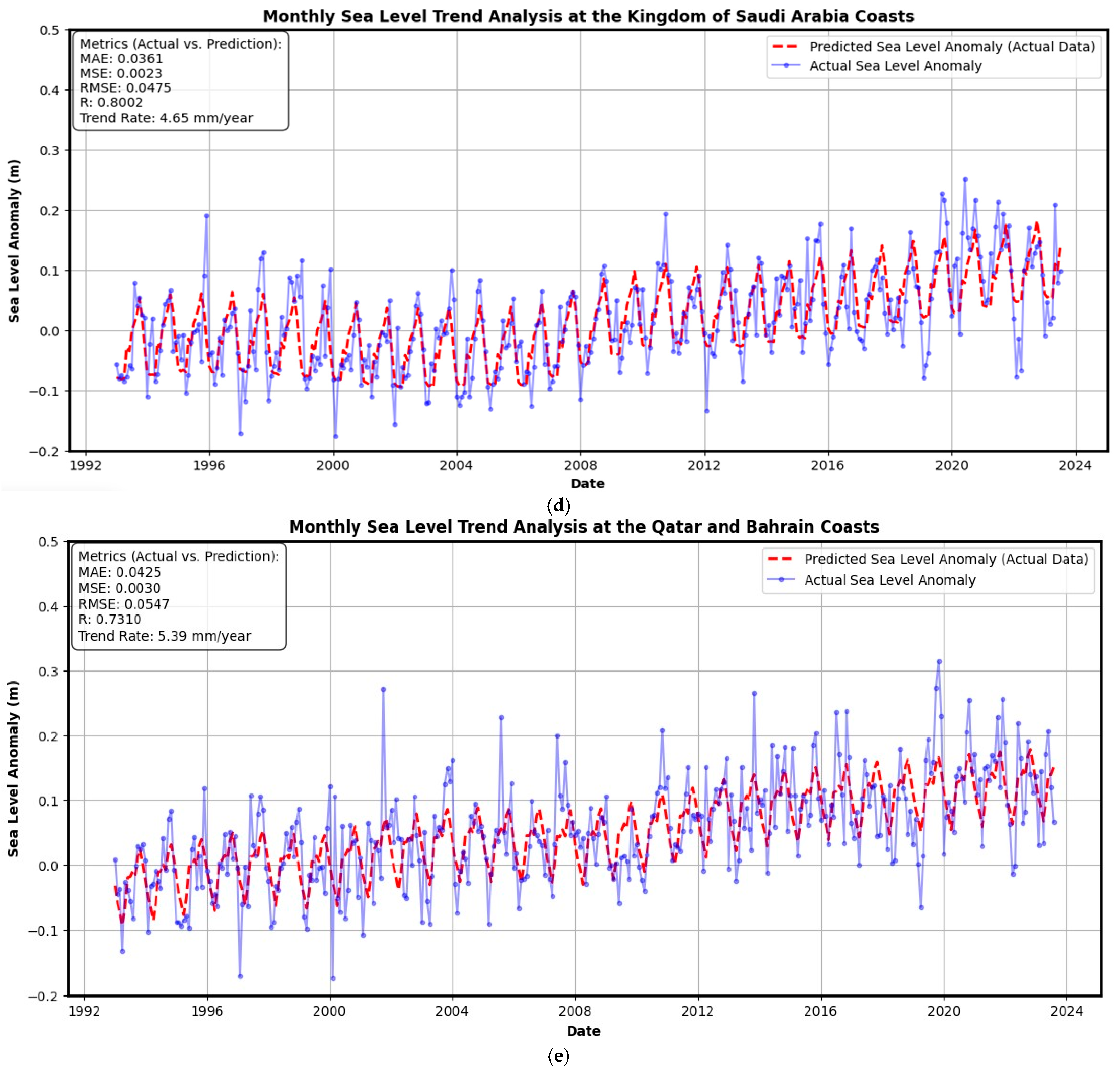
The variable, metrics, stores results from model training, like the cost function, error metrics, performance indicators, etc. The first ten rows of metrics show a performance summary for the model. With this script, Neural Prophet is trained with time-series data present in the DataFrame (df), and performance metrics are output to best fit the training data and assert the application of the model on new data. The Python script applies the fit() function after initialising the full Neural Prophet model in order to iteratively set the parameters for aligning the model with the time-series data. Throughout training, the method of stochastic gradient optimisation is employed by Neural Prophet to minimise the difference between forecasted and actual values. The highest absolute sea-level rise is envisaged by the prophet for the area of the Strait of Hormuz from 1993–2023, with the mean sea-level rise recorded as 5.23 mm/year at the station under consideration (Figure 6). The metric scores of MAE, MSE, RMSE, MAPE, and R² stand at 0.036, 0.002, 0.044, and 0.89, respectively. For the Iranian coast, the mean rise in sea level at the selected measurement point is 4.38 mm/year, while the values of the corresponding parameters are 0.0341, 0.002, 0.0437, and 0.8. Second comes Iraq–Kuwait with a rise of 4.46 mm/year, while the statistical measurements stand at 0.0456, 0.003, 0.0523, and 0.79. Saudi Arabia, on the other hand, stands at an average absolute sea-level rise of 4.41 mm/year, while the parameters are, respectively, 0.0361, 0.002, 0.047, and 0.87. Measurement stations along the Qatar and Bahrain coasts recorded an average of 4.29 mm/year, with statistical values of 0.0432, 0.002, 0.054, and 0.75, as shown in

Table 4. Summary of statistical metrics between actual and predicted sea level using Neural Prophet within the period of 1993 to 2023.

Region	MAE (m)	MSE (m2)	RMSE (m)	R2 Value	Sea-Level Rate (mm/Year)
Hormuz Straits	0.0364	0.002	0.0443	0.89	5.23
Iran coasts	0.0314	0.002	0.0437	0.8	4.38
Iraq and Kuwait coasts	0.0456	0.003	0.0523	0.79	4.46
Kingdom of Saudi Arabia coasts	0.0361	0.002	0.0471	0.87	4.41
Qatar and Bahrain coasts	0.0432	0.002	0.0536	0.75	4.29
UAE and Oman coasts	0.0421	0.003	0.0541	0.68	3.88
Average	0.0391	0.002	0.0492	0.8	4.44

. Finally, the UAE and Oman coasts exhibited the lowest rise, averaging 3.88 mm/year, with measures of 0.0421, 0.003, 0.0541, and 0.68, respectively.

Neural Prophet is logically better fitted to time-series analysis than simple or robust linear regression because linear models imply a unique and fixed linear trend and cannot interpret complicated time structures. Conversely, Neural Prophet splits the time-series into trend, seasonality, and noise terms, whereas the trend can vary gradually through a piecewise linear expression, thus reflecting gradual trends, seasonality, and interannual variability that define sea-level anomaly (SLA) records on a monthly basis, patterns that cannot be modeled sufficiently with a single straight line. This methodological benefit is well-evidenced in the quantitative outcome of the study whereby Neural Prophet had the highest average performance in all analysed regions, giving the lowest error measures (MAE = 0.0391 m and RMSE = 0.0492 m) and highest explanatory power (R² = 0.80) against simple linear regression (MAE = 0.052 m, RMSE = 0.066 m, and R² = 0.32) and robust regression (MAE). These findings can be associated with the approximate 25% decrease in error measures, as well as the significant increase in explanatory power. This is due to the fact that Neural Prophet is an interpretable hybrid model that is made up of time-series components which are additive and deep-learning features that are executed in PyTorch. The literature has shown that it has proven to be effective compared to the traditional Prophet model with different real-life time-series datasets [33]. Moreover, there are a number of applied papers that have demonstrated effective work with Neural Prophet on nonlinear time-series with seasonal variations, such as predicting solar-energy [40] and other applications related to dynamic systems [41]. Prophet-based models and other frameworks have been indicated as appropriate in the study of sea-level variability in conjunction with the same studies employing models based on machine learning and neural networks showing superior performance and hence stronger literature support in comparison with linear models [42], thus giving credence to the results of this research.

The observed rates of rising sea levels above the global average in the Persian Gulf can be viewed as a local manifestation of globally recorded climate-related sea-level change which is modulated by oceanographic and circulation processes on a basin scale. Human impact has been estimated by IPCC AR6 as the most significant cause of the measured rise in global mean sea level since at least 1971, mainly by ocean thermal expansion and loss of mass in land-iced masses. Contributions to the long-term sea-level change at the global scale include a glacial isostatic adjustment (GIA) of about 0.2–0.5 mm year⁻¹, highlighting this category of contribution at the global scale, which is often omitted in operational sea-level rise estimates so that the methodologies of satellite altimetry and tide-gauge records are consistent. Such a standardized structure incorporates the Sea Level Projection Tool of NASA, including IPCC AR6 projections, and shows that in 2020, the Persian Gulf had a higher surface sea-level increase of 45 mm per year⁻¹ than that of 1995–2014, supporting the notion of acceleration in similar decades. Simultaneously, global reference sea-level records realized using multi-mission satellite altimetry by CNES, as part of the AVISO programme, imposes common seasonal adjustments and temporal low-pass filters, uncovering spatially variant yet accelerating sea-level increase patterns across ocean basins. Here, the elevated rates in the Persian Gulf highlight the significance of scale-based assessments, or regional-level assessments, based on the fact that minor swings around the global average will result in disproportionately high coastal effects in low-gradient, shallow environments, which necessitates the importance of area-specific adaptation and coastal risk planning.

The findings of this study indicate the increasing contribution of data-driven techniques in the complement of traditional sea-level assessment techniques, especially in areas where in situ measurements and high-resolution physical models are sparse over time. Using the Neural Prophet model with the en bloc of the multi-decadal satellite altimetry measurements, this paper shows that machine-learning predictors are capable of delivering factual, consistent understanding of long-term sea-level behaviour and how this may change over time. Although these methods do not substitute the more physical-based climate or hydrodynamic models, these methods provide a viable decision-support system to determine relative trends, temporal variations, and realistic potential risk paths. In this regard, it is possible to note that the suggested methodology can be used to facilitate the support of early-stage coastal planning and prioritisation planning in the Persian Gulf and other low-relief coastal areas that are getting more and more vulnerable to sea-level rise.

4.3. Projection of Regional Sea-Level Rise Trend Using Prophet’s Model

The future prediction of the Persian Gulf sea level in this research is grounded on statistical extrapolation of the trends provided by the altimeter instead of physically constrained climate forecasting. These projections are conditional, scenario-instances of future extrapolation of statistically persistent behaviour of the sea-level behaviour seen throughout the satellite altimetry era (1993–2023) within a specified temporal horizon of up to 2100.

The sea-level time-series of the Persian Gulf can be well approximated as a linear trend over 30 years of records, including seasonal variability. Quadric and nonlinear formulations yielded tests with no statistically significant acceleration terms at a 95% confidence level, which means that acceleration cannot be determined with robustness based on the current record length. In both cases, therefore, the regression-based approaches yield a more or less linear long-term path, as well as the Prophet setup adopted here. Also, the Neural Prophet model in this paper was applied using a piecewise-linear trend formulation, which provides the ability to change the trend gradually but without the addition of physically inspired acceleration associated with forcing by greenhouse gases or cryospheric feedback. It is pointed out that such results are not to be taken as physically complete climate projections. They do not directly explain the variations in greenhouse gas emission, ice-sheet mass balance, or ocean circulation. Instead, they give a baseline projection based on conditioning on historical behaviour continuation and should be understood in parallel with scenario-based projections, like IPCC AR6.

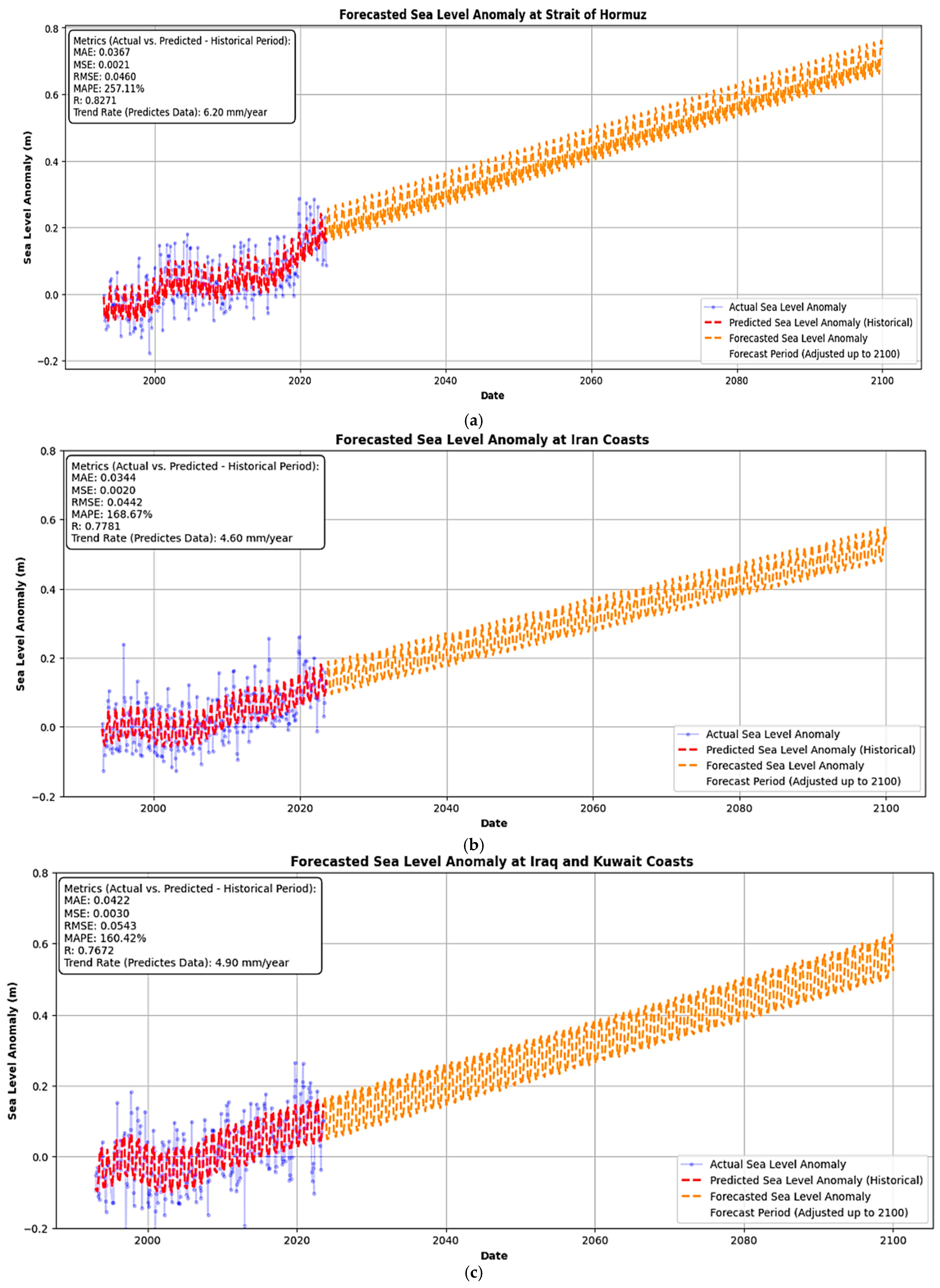
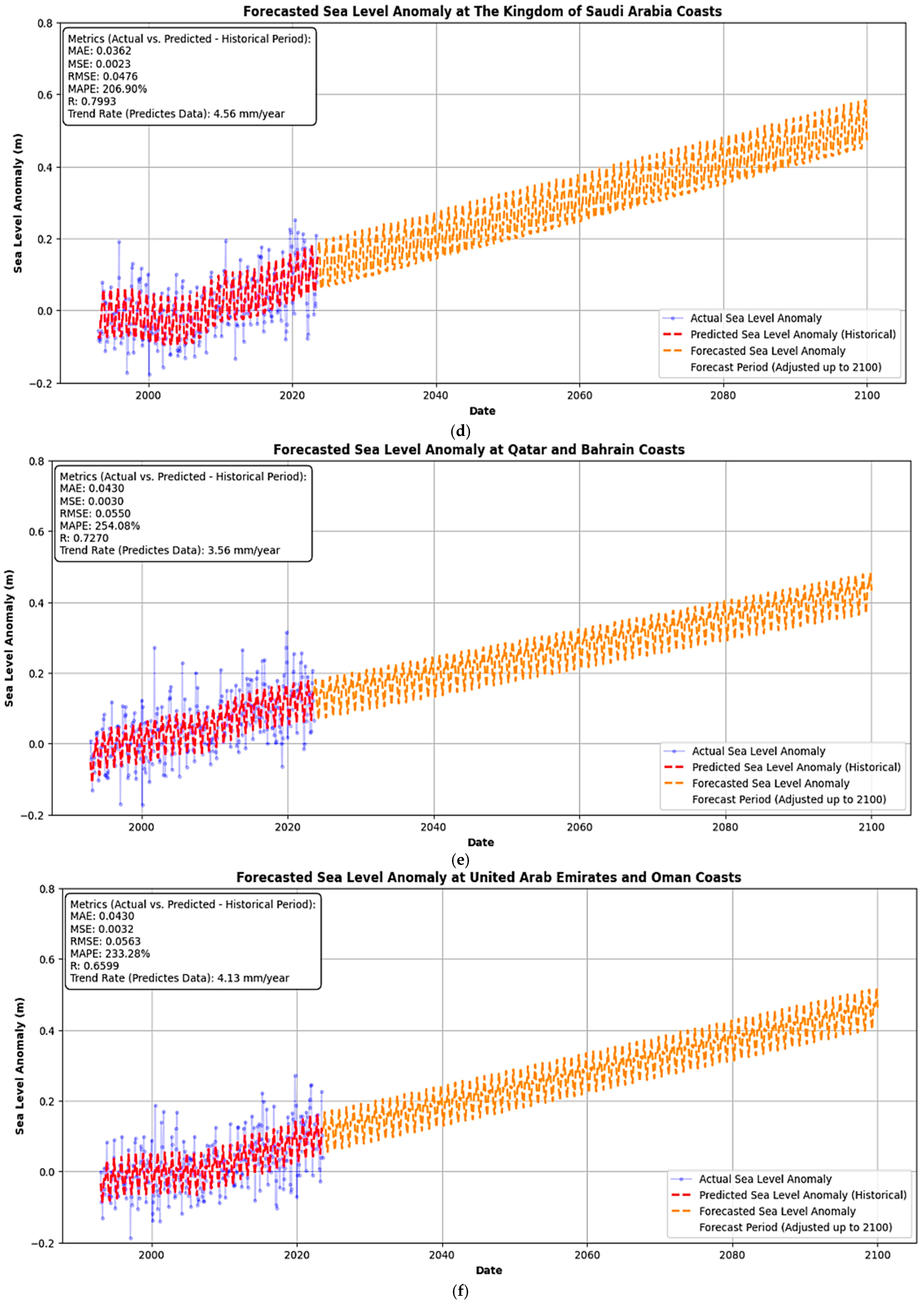
No statistically significant acceleration terms were found to have a 95-percent confidence level, meaning that the largest long-term sea-level signal during the course of observation is well characterized by a linear trend. In this regard, simple linear and robust regression models give a proper description of the data (first order) in a physical manner. The levels of uncertainty were measured by the 95% confidence limits of the slope of trend involving these regression equations and extrapolated to the estimated sea-level heights in 2040, 2060, 2080, and 2100. This was due to the application of Neural Prophet, which did not force nonlinear behaviour on the model; rather, it offered a flexible time-series model which can capture both linear behaviour trends and seasonal variability, as well as stochastic elements. The predictive uncertainty of Neural Prophet was estimated based on the internal uncertainty of the model, the output of which is the prediction intervals along with the median forecast. When acceleration is not statistically significant, Neural Prophet projections inherently approach almost linear extrapolation, as the regression results would do. The key projected sea-level trajectories are therefore tabulated in Figure 7, and the ranges of uncertainty are reported in numbers and discussed in the text instead of being represented graphically. On the whole, the mean increase in sea level in the Arabian Gulf by 2100 is projected to be in the range of about 0.30−0.40 m, with more in the Strait of Hormuz and less in the UAE–Oman coasts. These spatial variations indicate whole-basin circulation patterns and regional oceanographic forcing and largely conform to large-scale oceanographic evaluations. In real life, the findings show that the Persian Gulf in terms of sea level has been slowly increasing throughout the years during the observation period and that individual states along the coast show a variation. On overlaying these estimated sea-level shifts with elevation measurements taken at coastal areas, extensive lowlands (especially along flat and highly populated coasts) are evidenced as becoming more vulnerable to flooding. The spatial patterns that were determined in this research point at regions of priority that might be in need of adaptation efforts like coastal protection or land-use planning.

Figure 7 is a rundown of the Neural Prophet historical fitting and future forecasting of the six representative locations around the Persian Gulf of the mean sea-level anomaly up to the year 2100: the Strait of Hormuz, Iran coasts, Iraq coasts, Kuwait coasts, Saudi Arabia coasts, Qatar coasts, Bahrain coasts, and Oman coasts. It is estimated that the mean sea level is set to increase by 2100 to about 0.38–0.40 m in the Strait of Hormuz, 0.34–0.36 m in the Iran coasts, 0.35–0.37 m in the Iraq–Kuwait coasts, 0.33–0.35 m in the Saudi Arabia coasts, 0.29–0.31 m in the Qatar–Bahrain coasts, and 0.29–0.31 m in the UAE–Oman coasts, showing a definite increase. The high-performance metrics of low MAE and RMSE, small values of the MSE, low MAPE (usually not more than 5), and high coefficients of determination (R² = 0.75–0.90) in all the locations support the high convergence between observed and fitted values in every sub-figure (a–f). These findings validate that Neural Prophet is stable and useful in forecasting long-term sea-level changes and seasonal changes, hence it has strong ability and validity in long-term prediction of sea-level variations in the Persian Gulf.

Table 5. Mean of sea-level rise projections (in meters) around the Persian Gulf.

Persian Gulf	Year
	2040	2060	2080	2100
Hormuz Straits	0.089	0.194	0.298	0.403
Iran coasts	0.074	0.162	0.249	0.337
Iraq and Kuwait coasts	0.076	0.165	0.254	0.344
Kingdom of Saudi Arabia coasts	0.075	0.164	0.252	0.341
Qatar and Bahrain coasts	0.073	0.159	0.244	0.33
United Arab Emirates and Oman coasts	0.066	0.144	0.221	0.299

shows the future projections of the average height of the sea level in six Persian Gulf coastline areas at four-time projections (2040, 2060, 2080, and 2100) and indicates that the sea level significantly increases over the 21st century in all areas but with a near parallel slope. The Strait of Hormuz is the most proactive at all time steps with a high value of approximately 0.40 m projected by 2100 which indicates its excessive interaction with the open-ocean dynamics. The Iran and Iraq–Kuwait coasts come next with end-century rises of about 0.35–0.37 m, meaning that there is high susceptibility in the northern Gulf where the coastal topography is normally flat and low-lying. On the Saudi Arabia coasts, the sea level is estimated to increase consistently to about 0.34–0.35 m by the year 2100, indicating high long-term exposure in spite of less temporal fluctuations. The coasts of Qatar and Bahrain have slightly lower yet substantial increases, and they are expected to be about 0.32–0.33 m towards the end of the century. By far, the lowest projected values are noted in the UAE coasts, which are almost 0.30 m in 2100 but still show an evident positive trend. It is worth noting that even the mid-century projections (2040–2060) will show increases enough to increase tidal floodings, coastal erosion, and saltwater intrusion. Even with inter-regional differences in the order of a few centimetres, even these smaller differences can cause large differences in the inundation in low-gradient coastal environments. Generally, the Table 5 findings validate the strong spatial heterogeneity of sea-level rise throughout the Persian Gulf and sufficiently support a sound quantitative foundation of inundation models, exposure, and coastal adaptation, as well as region-specific models.

According to Table 5, the most projected increase in sea level is in the Strait of Hormuz (0.403 m by 2100). This is also in line with the fact that it is the deepest and most actively connected area of the Gulf, being the primary gateway of exchanging water with the Gulf of Oman where a decline in friction of the seabed and the robust exchange of the boundaries are instrumental in fully imparting the signals of the sea level [24]. The rest of the Persian Gulf is predominantly shallow, with an average depth of about 35 m [23]. The western and northern shelves are shallow and have increased bottom friction and shelf-dominated processes that attenuate and slow out the sea-level reaction. This geographic location concurs with a lower estimated sea-level rise that is experienced in other Gulf sub-regions, with ranges between 0.299–0.344 m.

Moreover, the semi-enclosed (characterized by limited interaction with the open sea), highly seasonal, and deep-water residence times of the Gulf allow for spatially coherent but non-uniform patterns of sea levels. Areas nearer to the open boundary (eastern Gulf and Hormuz) are more entrained to an open-ocean dynamic sea level and gradient pressure exchange effects, whilst the more distant interior shelves show a lessening dynamic response. The physical foundation of Table 5 is reinforced through this interpretation connection of the statistically identified regional variations to the known hydrodynamic controls, shallow-bathymetry modulation, and gateway-constrained exchange in the Gulf.

4.4. Validation of Satellite Altimetry Results

The accuracy of satellite altimetry in this study was validated by systematic comparison with high-quality tide-gauge observations from the Central Persian Gulf, using the Mina Salman (Bahrain) and Kangan (Iran) stations as reference benchmarks. These two stations were selected because many other regional tide gauges are affected by vertical instability, incomplete records, or questionable reliability, particularly those installed on offshore oil platforms, which introduce artificial sea-level signals due to platform subsidence, as mentioned in the Permanent Service for Mean Sea Level (PSMSL). In order to establish similarity between the datasets, monthly satellite sea-level anomalies (SLAs) were observed at sites close to the tide-gauge locations in the RADS multi-mission altimetry system. The two datasets were depth-reduced to the same mean sea-level (MSL) datum, and the anomalies obtained in the satellites could be easily compared to the in situ measurements. Each station was calculated as the mean value of the sea level over the long term and the individual tide-gauge anomaly as a deviation of the long-term mean to provide a common reference frame on which datasets can be compared. Statistical consistency between datasets was assessed by correlation and diagnostics of residual distributions. There was a high correlation between satellite altimetry and tide gauges at Mina Salman (R² = 0.761, STD = 0.029 m) and Kangan (R² = 0.741, STD = 0.041 m), indicating that satellite observations can accurately recreate the measured variability of the coastal sea level in the Persian Gulf.

The vertical land motion (VLM) of the Mina Salman station and Kangan station has been determined by calculating the difference in the trend between the tide-gauge and satellite altimetry (Tide Gauge (TG); Altimetry (ALT)). The estimated VLM rates at the Mina Salman are about −0.9 mm/year⁻¹ and at the Kangan, about −0.85 mm/year⁻¹, with the negative sign indicating a slight land uplift which causes the difference between the relative sea-level rise as recorded by the tide gauges and the absolute sea-level rise recorded by satellite-based altimetry. Since the TG trend estimates are uncertain (say between 1.30 mm/year and 1.95 mm/year at Mina Salman and Kangan, respectively), these values of VLM can only be taken as indicative and not absolute geodetic corrections, especially as the records are comparatively brief, and noisier values are usually found at the coast. On extrapolation to 2100 (supposing these rates of increase continue to apply rates as inferred in 2023), the forecast VLM is that of an extra relative sea-level difference of about 0.07 m at Mina Salman and 0.065 m at Kangan. These compensations, although slight relative to the regional average rates of change in the absolute sea level of about 4 mm year ⁻¹, can be used relative to the coastal effects and inundation analysis in low places. Notably, the deduced VLM magnitudes hold similar sign and magnitude comparisons with past GNSS-based research in the Arabian Gulf, including Al-Othmani (2014) [12], which indicated small vertical rates within the scale of ≤1 mm year at the Bahrain and Kuwait stations.

The computed rates of vertical land motion (VLM) based on the differences between the tide-gauge and the satellite altimetry trends (−0.9 mm/year–−0.85 mm/year) indicate the overall effective vertical land motion at the positions of the tide gauges and must not be deemed as a glacial isostatic adjustment (GIA) only. Vertical land movement is a product of a combination of several processes being added together, such as GIA, deformation of the Tectonics, compaction of sediments, and anthropogenic influence, but GIA is not the only part of the observed signal [43]. Since GIA is only a portion of the total VLM signal and site-specific GIA corrections are not applied directly in this work, the possible GIA contribution is instead solved by using a sensitivity framework by assuming a plausible GIA-related vertical rate of =−0.3 mm year⁻¹, in line with global GIA model estimates which do not include former ice-sheet regions [44,45]. Based on this assumption, GIA has been estimated to contribute to relative sea-level changes in the range of ±0.02–0.03 m by the year 2100. Despite its smallness in comparison with the estimated sea-level rise of the ocean, this contribution has been directly included in the uncertainty framework of interpretation in the coastal context. Vertical land motion (VLM) and glacial isostatic adjustment (GIA) corrections were not applied to the satellite altimetry records, as altimetry measures absolute sea-level changes in a geocentric reference frame. These corrections are relevant only for tide-gauge observations or when converting an absolute sea-level rise to a relative sea-level change in a coastal context.

4.5. Comparison with Global-Scale Sea-Level Rise Studies

The rates of the sea-level rise (SLR) obtained in this study have a high level of coherence with historical and modern data obtained at the regional and global levels. The Neural Prophet output shows that the Persian Gulf has an average SLR of 4.44 mm/year, with local peaks of over 5.2 mm/year at the Strait of Hormuz. NOAA (2025) and Abdulla and Al-Subhi (2021) both say that the basin is rising at an accelerated rate of 4.9 ± 0.4 mm/year and 4.29 mm/year, respectively [6,16]. Earlier studies using tide gauges found lower rates, such as 2.1 mm/year [8] and 2.42 mm/year [11]. These studies had small spatial coverage and low starting acceleration. Recent combinations of altimetry and tide gauges show a clear negative trend, with an estimate of 3.6 ± 0.4 mm/year [14], which matches the pattern noted here. It is acknowledged that there exists a methodological deficiency: Neural Prophet does not explicitly simulate greenhouse gas forcing or ice-sheet dynamics, resulting in predictions that are merely statistical extrapolations of observed behaviour rather than physics-based scenarios. However, the projected rise of about 0.30–0.40 m in the region is more in line with the intermediate pathways than the IPCC AR6 estimates of 0.43 m (SSP1–2.6) to 0.84 m (SSP5–8.5) at 2100 [46]. This shows that the global climate assessment is more accurate, but it is less accurate for the region. The integration of Neural Prophet outputs, satellite altimetry data, and IPCC AR6 scenario envelopes demonstrates that the Persian Gulf exhibits an accelerated rate of sea-level rise relative to global averages. The consistent regularity of these results enhances the model’s dependability and underscores the importance of local adaptation planning along the Gulf coastline. Neural Prophet does not explicitly offer greenhouse gas forcing, cryospheric dynamics, or steric expansion physics; therefore, forecasts are statistical extrapolations of observable patterns rather than scenario-driven climate simulations. Results were compared to IPCC AR6 scenarios to ensure conformity with physically based global projections.

Irrespective of its contributions, there are a number of limitations that this study warrants. The statistical extrapolation used to give the sea-level projections fails to explicitly reflect such things as the physical processes of climate change including ocean circulation, ice-sheet dynamics, or vertical land motion. Moreover, imprecision in digital elevation and topography of the coastline can affect the calculated area of inundation especially at the low-relief coastal areas. Although the hydrological approach of connectivity minimizes unrealistic inland floods, flooding flaws still continue to be a source of error. These constraints emphasise that the results should be interpreted as the possible risk cases but not deterministic predictions, and the results should be enhanced with future studies integrating physical modelling, better elevation estimates, and local subsidence measurements.

5. Conclusions

This study offers a regionally resolved evaluation of the present fluctuation and sea-level forecast in the Persian Gulf through a combination of three decades of homogenized multi-mission satellite altimetry and supplementary statistical and machine-learning systems. Instead of using the sparsely recorded tide gauges along the coast, or average sea-level behaviour estimates across a basin, the analysis measures sub-regional variations in how the basin responds to a long-term rise and shows coherent but spatially heterogeneous patterns of long-term rise behaviour. One of the main contributions of this work consists of the comparative analysis of linear, robust, and machine-learning-based trend formulations on the basis of uniform observational data. Although more traditional regression models are able to deliver explicit predictions of the first-order estimates of long-term sea-level rise, it is clear that Neural Prophet has distinct benefits in the non-stationary time evolution and seasonal organization of time, without any physical aids for acceleration. This concordance of independent methods of models makes it more certain that the observed trends are robust factors on a basin scale but not artifacts of plastic models. Geographically, the findings indicate that there is no spatial homogeneity in changing the sea level at the Persian Gulf, with the region being more sensitive at the Strait of Hormuz and less responsive to the shallow northern and western shelves. These characteristics are in agreement with established oceanographic conditions, such as limited exchange with the ocean, with bathymetry being shallow, and with high seasonal forcing hence the significance of regional-scale analysis in the transfer of global sea-level conditions to local risk evaluation. Even though the projections given here are statistical extrapolations given the historical behaviour, these can serve as a good baseline for near- and long-term coastal planning of regions where there are limited data. Combined with scenario-based climate predictions, this approach provides a pragmatic and reproducible system of determining regions of increased susceptibility, contributing to adaptation planning at an early phase and ranking coastal management interventions. This has a direct implication on the coastal management and policy formulation in the Persian Gulf region. To start with, the projections of high-risk inundation areas must receive priority in zoning regulations along the coastline, especially low-lying and hydrologically interdependent regions where even a slight rise in the sea level may lead to massive floods on inland regions. Second, long-term development strategies should include adaptation (setback lines, elevation-driven land-use planning, and strengthening of critical infrastructure corridors, e.g., ports, transportation networks, and energy facilities). Third, nature-based measures such as coastal wetlands and intertidal zone protection and restoration can offer affordable buffering to gradual sea-level rise along with other ecological advantages. Lastly, the results indicate the usefulness of incorporating satellite altimetry-based sea-level measurements and high-resolution elevation data into national risk assessment systems of coastal risks, which allows for re-assessing the risk of being submerged as new information is obtained. Despite the fact that the projections used in this paper are statistical and not physically based climate simulations, they offer plausible evidence demonstrating that near- to mid-term coastal adaptation planning needs to be conducted especially in data-sparse areas of the Persian Gulf.

In this study, three main types of data were employed to support the spatial and temporal analysis of sea-level variability. The first dataset (Supplementary S1) consists of satellite orbit route information, which was converted into a shapefile format and integrated within a Geographic Information System (GIS) environment to represent the spatial coverage of satellite observation tracks over the study area Figure 2. The second dataset (Supplementary S2) comprises Sea Level Anomaly (SLA) data derived from the Radar Altimeter Database System (RADS), which were utilised in Figure 5, Figure 6 and Figure 7 to analyse temporal sea-level variations and processed using the Google Colab platform. The third dataset (Supplementary S3) includes tide gauge station records, which were applied in Section 4.4 for the purpose of validating and cross-checking the satellite altimetry–derived sea-level measurements, thereby enhancing the reliability and robustness of the study results.

References

1. Melet, A.; van de Wal, R.; Amores, A.; Arns, A.; Chaigneau, A.A.; Dinu, I.; Haigh, I.D.; Hermans, T.H.J.; Lionello, P.; Marcos, M.; et al. Sea Level Rise in Europe: Observations and projections. In Sea Level Rise in Europe: 1st Assessment Report of the Knowledge Hub on Sea Level Rise (SLRE1); van den Hurk, B., Pinardi, N., Kiefer, T., Larkin, K., Manderscheid, P., Richter, K., Eds.; Copernicus Publications: Göttingen, Germany, 2024. [Google Scholar] [CrossRef]
2. Luijendijk, A.; Hagenaars, G.; Ranasinghe, R.; Baart, F.; Donchyts, G.; Aarninkhof, S. The State of the World’s Beaches. Sci. Rep. 2018, 8, 6641. [Google Scholar] [CrossRef]
3. Mentaschi, L.; Vousdoukas, M.I.; Pekel, J.-F.; Voukouvalas, E.; Feyen, L. Global long-term observations of coastal erosion and accretion. Sci. Rep. 2018, 8, 12876. [Google Scholar] [CrossRef]
4. Addo, K.A.; Addo, I.A. Coastal erosion management in Accra: Combining local knowledge and empirical research. J. Disaster Risk Stud. 2016, 8, 274. [Google Scholar] [CrossRef]
5. IPCC. Climate Change 2021: The Physical Science Basis Contribution of Working Group I to the Sixth Assessment Report of the Intergovernmental Panel on Climate Change; Masson-Delmotte, V.P., Zhai, A., Pirani, S.L., Connors, C., Péan, S., Berger, N., Caud, Y., Chen, L., Goldfarb, M.I., Gomis, M., et al., Eds.; Cambridge University Press: Cambridge, UK, 2021. [Google Scholar] [CrossRef]
6. NOAA. Ocean Topography and Cryosphere Branch/Laboratory for Satellite Altimetry/Sea Level Rise. 2025. Available online: https://www.star.nesdis.noaa.gov/socd/lsa/SeaLevelRise/LSA_SLR_timeseries_regional.php (accessed on 1 January 2025).
7. NASA. IPCC 6th Assessment Report Sea Level Projections Tool. 2025. Available online: https://sealevel.nasa.gov/ipcc-ar6-sea-level-projection-tool (accessed on 1 January 2025).
8. Sultan, S.A.R.; Ahmad, F.; Elghribi, N.M.; Al-Subhi, A.M. An analysis of Arabian Gulf monthly mean sea level. Cont. Shelf Res. 1996, 15, 1471–1482. [Google Scholar] [CrossRef]
9. Sultan, S.A.R.; Moamar, M.O.; El-Ghribi, N.M.; Williams, R. Sea level changes along the Saudi Coast of the Arabian Gulf Indian. J. Mar. Sci. 2000, 29, 191–200. [Google Scholar]
10. Hassanzadeh, S.; Kiasatpour, A.; Hosseinibalam, F. Sea-level response to atmospheric forcing along the north coast of Persian Gulf. Meteorol. Atmos. Phys. 2007, 95, 223–237. [Google Scholar] [CrossRef]
11. Alothman, A.O.; Ayhan, M.E.; Arabia, S. Detection of sea level rise within the Arabian Gulf using space based GNSS measurements and insitu tide gauge data: Preliminary results. In Change, Impacts, Vulnerability & Adaptation; Environment Agency-Abu Dhabi: Abu Dhabi, United Arab Emirates, 2010. [Google Scholar]
12. Alothman, A.O.; Bos, M.S.; Fernandes, R.M.S.; Ayhan, M.E. Sea level rise in the north-western part of the Arabian Gulf. J. Geodyn. 2014, 81, 105–110. [Google Scholar] [CrossRef]
13. Shehadi, M.A. Vulnerability of Mangroves to Sea Level Rise in Qatar: Assessment and Identification of Vulnerable Mangroves Areas. Master’s Thesis, Qatar University, Doha, Qatar, 2015. [Google Scholar]
14. Siddig, N.A.; Al-Subhi, A.M.; Alsaafani, M.A. Tide and mean sea level trend in the west coast of the Arabian Gulf from tide gauges and multi-missions satellite altimeter. Oceanologia 2019, 61, 401–411. [Google Scholar] [CrossRef]
15. Siddig, N.A.; Al-Subhi, A.M.; Alsaafani, M.A.; Alraddadi, T.M. Applying Empirical Orthogonal Function and Determination Coefficient Methods for Determining Major Contributing Factors of Satellite Sea Level Anomalies Variability in the Arabian Gulf. Arab. J. Sci. Eng. 2021, 47, 619–628. [Google Scholar] [CrossRef]
16. Abdulla, C.P.; Al-Subhi, A.M. Is the Red Sea Sea-Level Rising at a Faster Rate than the Global Average? An Analysis Based on Satellite Altimetry Data. Remote Sens. 2021, 13, 3489. [Google Scholar] [CrossRef]
17. Albanai, J. Sea level rise projections for Failaka Island in the State of Kuwait. Trans. Marit. Sci. 2020, 9, 236–247. [Google Scholar] [CrossRef]
18. Barbosa, S.M.; Silva, M.E.; Fernandes, M.J. Long-term sea level variability: A statistical approach using time series analysis. J. Geophys. Res. Ocean. 2008, 113, C11010. [Google Scholar] [CrossRef]
19. Hyndman, R.J.; Athanasopoulos, G. Forecasting: Principles and Practice, 2nd ed.; OTexts: Melbourne, Australia, 2018; Available online: https://otexts.com/fpp2/ (accessed on 1 January 2025).
20. Bahari, N.A.A.B.S.; Ahmed, A.N.; Chong, K.L.; Lai, V.; Huang, Y.F.; Koo, C.H.; Ng, J.L.; El-Shafie, A. Predicting Sea Level Rise Using Artificial Intelligence: A Review. Arch. Comput. Methods Eng. 2023, 30, 4045–4062. [Google Scholar] [CrossRef]
21. Rajabi-Kiasari, S.; Delpeche-Ellmann, N.; Ellmann, A.; Soomere, T. Forecasting sea level maxima using Machine learning with explainability and extreme value analysis. Int. J. Appl. Earth Obs. Geoinf. 2026, 146, 105064. [Google Scholar] [CrossRef]
22. Uluocak, I. Comparative study of multivariate hybrid neural networks for global sea level prediction through 2050. Environ. Earth Sci. 2025, 84, 79. [Google Scholar] [CrossRef]
23. Reynolds, R.M. Physical oceanography of the Persian Gulf, Strait of Hormuz, and the Gulf of Oman. Mar. Pollut. Bull. 1993, 27, 35–59. [Google Scholar] [CrossRef]
24. Sheppard, C.; Al-Husiani, M.; Al-Jamali, F.; Al-Yamani, F.; Baldwin, R.; Bishop, J.; Benzoni, F.; Dutrieux, E.; Dulvy, N.K.; Durvasula, S.R.V.; et al. The Gulf: A young sea in decline. Mar. Pollut. Bull. 2010, 60, 13–38. [Google Scholar] [CrossRef]
25. Swift, S.A.; Bower, A.S. Formation and circulation of dense water in the Persian Gulf. J. Geophys. Res. Ocean. 2003, 108, 3004. [Google Scholar] [CrossRef]
26. Yao, F.; Johns, W.E. A HYCOM modeling study of the Persian Gulf: 1. Model configuration and surface circulation. J. Geophys. Res. Ocean. 2010, 115, C11017. [Google Scholar] [CrossRef]
27. Schrama, E.J.O. The Role of Orbit Errors in Processing of Satellite Altimeter Data; Publications on Geodesy, New Series, No. 33; Netherlands Geodetic Commission: Delft, The Netherlands, 1989; ISBN 90-6132-239. [Google Scholar]
28. Trisirisatayawong, I.; Naeije, M.; Simons, W.; Fenoglio-Marc, L. Sea level change in the Gulf of Thailand from GPS-corrected tide gauge data and multi-satellite altimetry. Glob. Planet. Change 2011, 76, 137–151. [Google Scholar] [CrossRef]
29. Andersen, O.B.; Scharroo, R. Range and geophysical corrections in coastal regions: And implications for mean sea surface determination. In Coastal Altimetry; Springer: Berlin/Heidelberg, Germany, 2011; pp. 103–145. [Google Scholar]
30. Samuels, P.; Gilchrist, M. Simple Linear Regression; Cambridge University Press: Cambridge, UK, 2014; Available online: https://www.researchgate.net/publication/275018503_Simple_Linear_Regression (accessed on 1 January 2025).
31. Holland, P.W.; Welsch, R.E. Robust regression using iteratively reweighted leastsquares. Commun. Stat.-Theory Methods 1977, 6, 813–827. [Google Scholar] [CrossRef]
32. Taylor, S.J.; Letham, B. Forecasting at scale. Am. Stat. 2017, 72, 37–45. [Google Scholar] [CrossRef]
33. Triebe, O.; Hewamalage, H.; Pilyugina, P.; Laptev, N.; Bergmeir, C.; Rajagopal, R. NeuralProphet: Explainable Forecasting at Scale. arXiv 2021, arXiv:2111.15397. [Google Scholar] [CrossRef]
34. Hyndman, R.J.; Athanasopoulos, G. Forecasting: Principles and Practice, 3rd ed.; OTexts: Melbourne, Australia, 2021; Available online: https://OTexts.com/fpp3 (accessed on 1 January 2025).
35. Haris, M.D.; Adytia, D.; Ramadhan, A.W. Air temperature forecasting with long short-term memory and prophet: A case study of Jakarta, Indonesia. In Proceedings of the 2022 International Conference on Data Science and Its Applications (ICoDSA), Bandung, Indonesia, 6–7 July 2022; pp. 251–256. [Google Scholar] [CrossRef]
36. Toharudin, T.; Pontoh, R.S.; Caraka, R.E.; Zahroh, S.; Lee, Y.; Chen, R.C. Employing long short-term memory and Facebook prophet model in air temperature forecasting. Commun. Stat. Simul. Comput. 2023, 52, 279–290. [Google Scholar] [CrossRef]
37. Das, N.; Sagar, A.; Bhattacharjee, R.; Agnihotri, A.K.; Ohri, A.; Gaur, S. Time series forecasting of temperature and turbidity due to global warming in river ganga at and around Varanasi, India. Environ. Monit. Assess. 2022, 194, 617. [Google Scholar] [CrossRef]
38. Elseidi, M. A hybrid Facebook prophet-ARIMA framework for forecasting high-frequency temperature data. Model. Earth Syst. Environ. 2024, 10, 1–13. [Google Scholar] [CrossRef]
39. Din, A.H.M. Sea Level Rise Estimation and Interpretation in Malaysian Region Using Multi-Sensor Techniques. Ph.D. Thesis, Universiti Teknologi Malaysia, Johor Bahru, Malaysia, 2014. [Google Scholar]
40. Arias Velásquez, R.M. A case study of NeuralProphet and nonlinear evaluation for high-accuracy short-term forecasting in a photovoltaic solar plant. Heliyon 2022, 8, e10437. [Google Scholar] [CrossRef]
41. Tahir, H.; Din, A.H.M.; Hussein, T.S. Future Coastal Inundation Risk Map for Iraq by the Application of GIS and Remote Sensing. Earth 2026, 7, 8. [Google Scholar] [CrossRef]
42. Sinha, S.; Fasullo, J.; Nerem, R.S.; Monteleoni, C. Multidecadal Sea Level Prediction Using Neural Networks and Spectral Clustering on Climate Model Large Ensembles and Satellite Altimeter Data. Artif. Intell. Earth Syst. 2024, 3, e230089. [Google Scholar] [CrossRef]
43. Hammond, W.C.; Blewitt, G.; Li, Z.; Plag, H.-P.; Kreemer, C. GPS imaging of global vertical land motion for studies of sea level rise. J. Geophys. Res. Solid Earth 2021, 126, e2021JB022355. [Google Scholar] [CrossRef]
44. Peltier, W.R. Global glacial isostasy and the surface of the ice-age Earth: The ICE-5G(VM2) model and GRACE. Annu. Rev. Earth Planet. Sci. 2004, 32, 111–149. [Google Scholar] [CrossRef]
45. Spada, G. Glacial isostatic adjustment and contemporary sea level rise: An overview. Surv. Geophys. 2017, 38, 153–185. [Google Scholar] [CrossRef]
46. IPCC. Climate Change 2022: Impacts Adaptation, and Vulnerability Contribution of Working Group II to the Sixth Assessment Report of the Intergovernmental Panel on Climate Change; Pörtner, H.-O., Roberts, D.C., Tignor, M., Poloczanska, E.S., Mintenbeck, K., Alegría, A., Craig, M., Langsdorf, S., Löschke, S., Möller, V., et al., Eds.; Cambridge University Press: Cambridge, UK; New York, NY, USA, 2022; p. 3056. [Google Scholar] [CrossRef]
Figure 1. Case study.
Geomatics 06 00009 g001
Figure 2. Altimeter tracks of Jason-1/2/3, Topex, Envisat, Sentinel6_MF, Saral, ERS1/2, and GFO for the Persian Gulf.
Geomatics 06 00009 g002
Figure 3. The location of altimeter grid points used in this study (blue colour) to derive sea-level anomalies for four areas over the Persian Gulf.
Geomatics 06 00009 g003
Figure 4. Sea-level anomaly prediction methodology by three models.
Geomatics 06 00009 g004
Figure 5. The analysis of monthly sea-level trends for (a) the Strait of Hormuz (Lat: 26.25, Long: 56.00), (b) Iran coasts (Lat: 27.75, Long: 52), (c) Iraq and Kuwait coasts (Lat: 28.75, Long: 49.00), (d) Kingdom of Saudi Arabia coasts (Lat: 28.00, Long: 50.25), (e) Qatar and Bahrain coasts (Lat: 26.5, Long: 51.50), and (f) United Arab Emirates and Oman coasts (Lat: 26, Long: 56.5) using the robust fit regression technique with linear trends superimposed with a red line, whereas the simple fit regression technique is superimposed with a blue line. MAE and RMSE retain the same physical unit as the original measurements (meters), while MSE is expressed in squared units (m2) because it is computed as the mean of squared residuals.
Geomatics 06 00009 g005aGeomatics 06 00009 g005bGeomatics 06 00009 g005c
Figure 6. Monthly sea-level trend analysis for (a) the Strait of Hormuz at (Lat: 26.25, Long: 56.00), (b) Iran coasts at (Lat: 27.75, Long: 52), (c) Iraq and Kuwait coasts at (Lat: 28.75, Long: 49.00), (d) Kingdom of Saudi Arabia coasts at (Lat: 28.00, Long: 50.25), (e) Qatar and Bahrain coasts at (Lat: 26.5, Long: 51.50), and (f) United Arab Emirates and Oman coasts at (Lat: 26, Long: 56.5) by Neural Prophet. MAE and RMSE retain the same physical unit as the original measurements (meters), while MSE is expressed in squared units (m2) because it is computed as the mean of squared residuals.
Geomatics 06 00009 g006aGeomatics 06 00009 g006bGeomatics 06 00009 g006cGeomatics 06 00009 g006d
Figure 7. Forecasted mean sea-level trends for (a) the Strait of Hormuz at (Lat: 26.25, Long: 56.25), (b) Iran coasts at (Lat: 27.75, Long: 52), (c) Iraq and Kuwait coasts at (Lat: 29.5, Long: 48.75), (d) Kingdom of Saudi Arabia coasts at (Lat: 28, Long: 49.25), (e) Qatar and Bahrain coasts at (Lat: 25, Long: 51.75), and (f) United Arab Emirates and Oman coasts at (Lat: 26, Long: 56.5) by Neural Prophet. Evaluation metrics (MSE) are stated in squared units (m2) as derived from squared residuals, while MAPE is unitless and provided as a percentage (%) to reflect relative error magnitude. MAE and RMSE use the same physical unit as observations (meters).
Geomatics 06 00009 g007aGeomatics 06 00009 g007b