Article

An Integrated Remote Sensing and Machine Learning Approach to Assess the Impact of Soil Salinity on Rice Yield in Northeastern Thailand

by
Jurawan Nontapon
1,
Neti Srihanu
2,
Niwat Bhumiphan
3,
Nopanom Kaewhanam
1,
Anongrit Kangrang
1,
Umesh Bhurtyal
4,
Niraj KC
5,
Siwa Kaewplang
1,* and
Alfredo Huete
6
1
Faculty of Engineering, Mahasarakham University, Kantharawichai District, Maha Sarakham 44150, Thailand
2
Faculty of Engineering, Northeastern University, Khon Kaen 40000, Thailand
3
Faculty of Technology and Engineering, Udon Thani Rajabhat University, Sam Phrao Subdistrict, Mueang District, Udon Thani 41000, Thailand
4
Department of Geomatics Engineering, Pashchimanchal Campus, Tribhuvan University, Kaski 33700, Nepal
5
Institute of Engineering and IT, Lumbini Technological University (LTU), Nepalgunj 21900, Nepal
6
School of Life Sciences, University of Technology Sydney, Sydney, NSW 2007, Australia
*
Author to whom correspondence should be addressed.
Geomatics 2025, 5(4), 80; https://doi.org/10.3390/geomatics5040080
Submission received: 6 September 2025 / Revised: 23 November 2025 / Accepted: 9 December 2025 / Published: 13 December 2025

Abstract

The Northeast region of Thailand covers approximately 16.89 million hectares, with about 6.17 million hectares of seasonal rice cultivation and 2.85 million hectares affected by soil salinity—a major constraint to agricultural productivity in this region. This study develops an integrated data fusion framework combining multi-temporal Landsat-8 and Sentinel-2 imagery to train machine learning (ML) models for the prediction of rice yield and soil salinity, allowing for an analysis of their relationship. The field data comprised 380 rice yield and 625 soil electrical conductivity (EC) samples collected in 2023. Three ML models—Random Forest (RF), Classification and Regression Trees (CART), and Support Vector Regression (SVR)—were applied for variable reduction and optimal predictor selection. RF achieved the highest accuracy for yield prediction (R2 = 0.86, RMSE = 0.19 t ha−1) and salinity estimation (R2 = 0.93, RMSE = 0.87 dS/m) when using fused Landsat–Sentinel data. Spatial analysis of 5000 matched points showed a strong negative relationship between seedling stage EC and yield (R2 = 0.71), with yields declining sharply above 5 dS/m and remaining below 1.5 t ha−1 beyond 15 dS/m. These results demonstrate the potential of multi-sensor fusion and ensemble ML approaches for precise soil salinity monitoring and sustainable rice production.

1. Introduction

Soil salinity is a critical global issue, affecting over 20% of irrigated lands due to both natural processes and human activities [1]. Aggravated by climate change and the mismanagement of water and land resources, it leads to declining crop yields and land degradation [2]. Globally, soil salinity and alkalinity threaten agricultural sustainability and food security, particularly in arid and semi-arid regions.
Rice (Oryza sativa L.), one of the world’s most important staple crops, is highly sensitive to salt stress. Excess salinity disrupts osmotic balance and nutrient uptake, inhibiting germination, tillering, and grain filling [3,4,5]. During dry seasons, strong evaporation and inadequate drainage accelerate salt accumulation on the soil surface, severely reducing productivity in paddy fields [6,7,8]. Empirical studies have shown that rice yield declines sharply when soil electrical conductivity (ECe) exceeds 3.0 dS/m, with further reductions observed between 3.9 and 6.5 dS/m [9,10,11]. Although improved rice varieties, nutrient management [12], and irrigation adjustments [13] have mitigated salinity impacts, efficient and large-scale monitoring of salinity stress remains a persistent challenge.
Field-based salinity assessments are accurate but spatially limited and resource-intensive. Remote sensing (RS) provides a scalable alternative, enabling continuous monitoring of crop growth and soil conditions. Previous studies successfully used vegetation indices such as NDVI and EVI derived from Landsat, Sentinel, and MODIS imagery to estimate rice yield with high precision (R2 > 0.8, RMSE = 0.18–0.25 t ha−1) [14,15,16,17,18,19,20,21]. When integrated with ML algorithms such as RF, SVR, and Artificial Neural Networks (ANNs), these approaches effectively captured nonlinear relationships between spectral features and yield outcomes [17,18,19,20].
Multi-source remote sensing has progressed rapidly. Integrating optical and radar data (MODIS, Sentinel-1, Landsat-8, Sentinel-2) with ML models (RF, CatBoost) and fusion techniques (STARFM, FSDAF) enhances yield prediction (R2 = 0.70–0.89; RMSE < 0.5 t ha−1) [22,23,24,25,26], while deep learning models (BiLSTM, U-Net) using Sentinel-1 time series achieved superior accuracy (R2 = 0.92–0.98) [27]. These achievements have established ML–RS integration as a robust framework for agricultural yield prediction. The ensemble architecture of the Random Forest (RF) model enables the integration of signals from multiple spectral regions (red, green, and NIR) and effectively captures nonlinear relationships between plant stress and spectral reflectance [28,29]. Parallel advancements have been achieved in soil salinity estimation. Studies employing Landsat-8 and Sentinel-2 imagery combined with spectral indices—such as the Salinity Index (SI), NDSI, and COSRI—and ML algorithms have reported strong performance (R2 = 0.67–0.98; RMSE = 1.8–7.3 dS/m) [24,30,31,32,33,34,35,36,37,38]. Aksoy et al. [29] found that the CART model achieved R2 = 0.98 using Sentinel-2A data, while Haq et al. [32] showed that RF performed best (R2 = 0.94, RMSE = 1.89 dS/m). These studies demonstrate the high potential of satellite–ML approaches for accurate soil salinity mapping. More recent research integrating optical, radar, thermal, and terrain features with ML algorithms (RF, SVR, CNN) further improved mapping accuracy to R2 up to 0.96 [35,36,37].
However, most existing studies have treated rice yield prediction and soil salinity mapping as independent research topics, thereby overlooking their mutual influence. As a result, the physiological mechanisms linking salinity stress to yield reduction—such as osmotic imbalance, chlorophyll degradation, and biomass suppression—remain poorly represented in remote sensing-based models. Additionally, tropical paddy systems, which experience dynamic interactions between monsoonal flooding, evaporation, and irrigation, have received far less attention than arid or coastal environments. A systematic framework that jointly quantifies these relationships is still lacking.
To bridge these gaps, this study proposes an integrated remote sensing and machine learning framework that simultaneously predicts rice yield and soil electrical conductivity (EC) using fused Sentinel-2 and Landsat-8 imagery. Three ML algorithms—RF, SVR, and CART—were employed to assess the predictive performance of spectral indices related to vegetation and salinity. By interpreting machine learning variable importance in terms of crop physiological stress, the framework establishes a novel spectral–physiological linkage that connects canopy reflectance with underlying salinity-induced processes.
This study is among the first to jointly model rice yield and soil salinity within a tropical paddy ecosystem, providing an integrated perspective on their bidirectional interactions. Furthermore, the fusion of Sentinel-2 and Landsat-8 data enhances both spatial resolution and predictive robustness, enabling scalable applications for precision agriculture, salinity risk mapping, and sustainable land management across tropical rice-growing regions. Therefore, this study contributes to bridging the gap between crop physiology and remote sensing-based modeling through a unified framework for tropical rice ecosystems. The specific objectives are to:
(i)
evaluate the effectiveness of time-series Sentinel-2 and Landsat-8 data combined with vegetation indices (NDVI, EVI) and ML algorithms for rice yield prediction;
(ii)
assess the integration of Sentinel-2 and Landsat-8 with salinity-related indices for EC estimation; and
(iii)
examine how soil salinity during the seedling stage affects rice yield.

2. Method

2.1. Study Area

The study area is located in Northeast Thailand (14°09′55″–18°26′50″ N, 101°23′50″–105°38′35″ E) (Figure 1), which covers approximately 16.89 million hectares and represents the country’s largest agricultural region. This area is characterized by gently undulating terrain and diverse agro-climatic conditions across the Korat Plateau. The elevation ranges from 62 to 213 m above sea level, descending from the Phetchabun Mountains in the west to the Mekong River in the east. The region is divided into two major plains: the southern Korat Plain (drained by the Mun and Chi rivers) and the northern Sakon Nakhon Plain (drained by the Loei and Songkhram rivers), separated by the Phu Phan Mountains. The climate is tropical savanna, with average annual temperatures ranging from 19.6 °C to 30.2 °C. Precipitation ranges between 1270 and 2000 mm, mostly concentrated during the May–October rainy season and presenting an uneven rainfall distribution. The Northeast region of Thailand is predominantly characterized by sandy soils, leading to low fertility and high susceptibility to erosion. These factors contribute to lower agricultural productivity compared with other regions of the country. Approximately 2.85 million hectares (16.7%) of the study area are affected by soil salinity [39], comprising 1.41% highly saline soils, 3.47% moderately saline soils, and 11.8% slightly saline soils. In addition, approximately 3.10 million hectares (18.2%) are at risk of further salinization. Most soils are sandy with underlying salt bearing layers, which exacerbate salinity problems during the dry season and particularly affect rice growth during the reproductive stages. The Northeast plays a vital role in national rice production, accounting for more than 60% of the country’s seasonal rice cultivation area (≈6.17 million hectares) and producing 12–14 million tons annually. Consequently, soil salinity represents a major threat to rice productivity and the security of farmers’ livelihoods in this region. The map of soil salt-crust distribution in Northeast Thailand shown in Figure 1 was kindly provided in shapefile format by the Land Development Department (LDD), Ministry of Agriculture and Cooperatives, Thailand, under the data-sharing policy for academic and research purposes. The dataset can be requested through the official website at http://sql.ldd.go.th/ldddata/mapsoilA8.html, accessed on 10 February 2024.

2.2. Rice Growth Phenology and the Role of Vegetation Indices NDVI and EVI

According to the crop calendar, rainfed rice in Northeastern Thailand typically follows a growth cycle from planting in June–July to harvesting in December. The crop progresses through four main stages—nursery, vegetative, reproductive, and maturity—lasting approximately 5–6 months, depending on the rice variety and environmental conditions [40,41].
Throughout this cycle, the crop’s spectral reflectance changes and NDVI and EVI values increase during the Greenup stage and peak in October during the heading phase. These values then stabilize or decline during the ripening stage, due to reduced leaf area and stem moisture. Maturity is reached in November, and harvest takes place in December (see Figure 2 for details). Vegetation indices such as NDVI and EVI are widely utilized for monitoring the growth stages of rice [19,42]. NDVI remains low during early development due to sparse vegetation, then increases with chlorophyll accumulation and canopy expansion. Near-infrared reflectance rises as foliage and tillers develop, but NDVI declines at maturity due to biomass reduction and grain filling [43]. However, NDVI tends to saturate in dense vegetation, making it less effective in characterizing later stages. EVI was developed to overcome this limitation by reducing saturation and improving the correlation with biomass [44]. While NDVI is useful for early-stage monitoring, EVI performs better in areas with high vegetation density by correcting for atmospheric effects and background noise. Therefore, the choice between NDVI and EVI depends on the growth stage and environmental conditions, with EVI offering better distinction in later, denser stages [45].

2.3. Field Data Collection Strategy

2.3.1. Rice Yield Ground Truth Data Collection

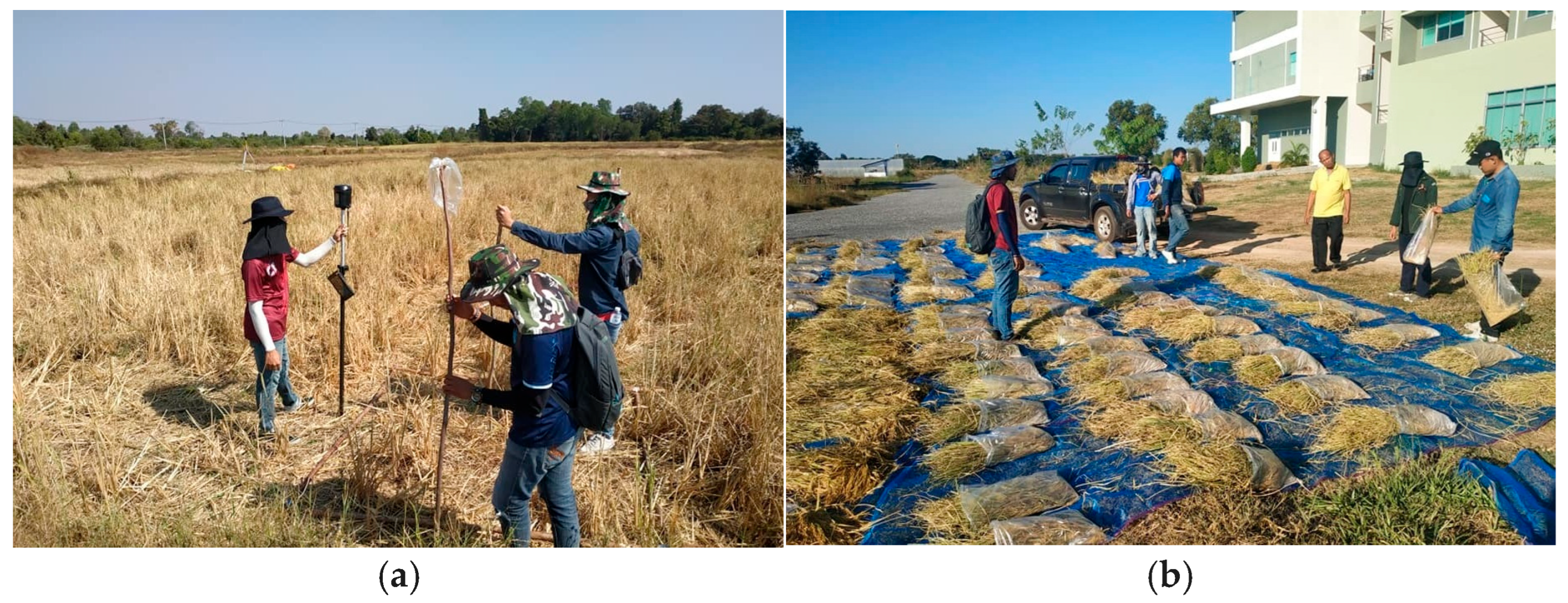
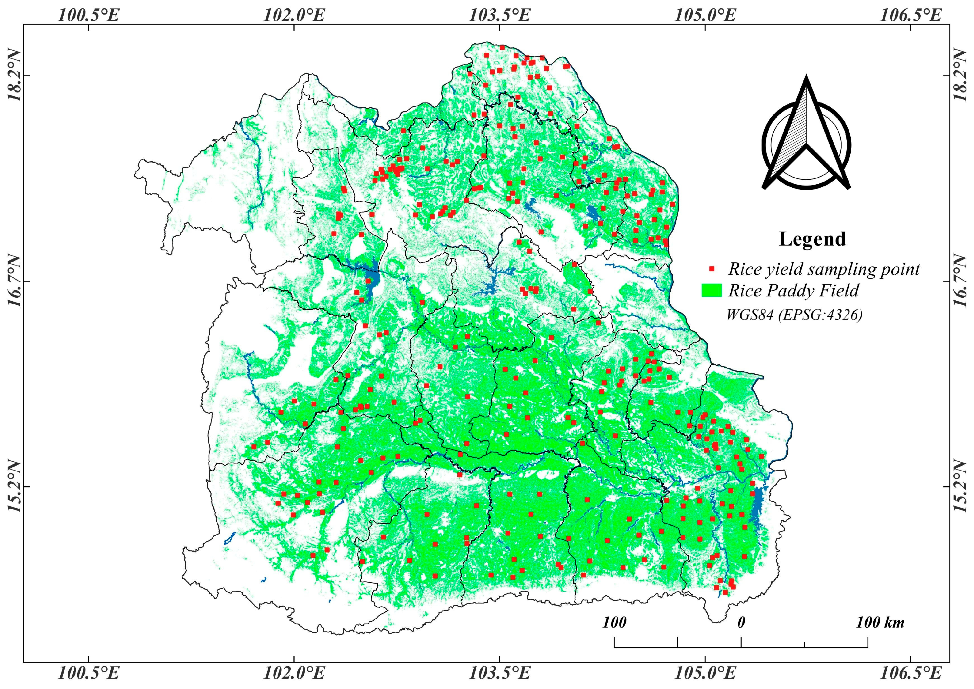
A total of 380 rice yield samples were collected from farm plots harvested between November and December 2023, each covering at least 0.8 hectares to ensure yield representativeness. Plot locations were recorded using RTK GNSS with sub 5 cm accuracy, reducing spatial error and improving alignment with environmental variables such as soil salinity (Figure 3a). Yield data were obtained using a standard post-harvest field weighing method, with plot selection designed to capture variation in salinity conditions. Sample preparation, including sorting and weighing procedures, was conducted uniformly across all plots (Figure 3b). In addition, field data collection was supported by several private rice mills in the area, which facilitated comprehensive and reliable data acquisition. The dataset, compiled at the farm plot level, was used for modeling and validation purposes. The wide spatial distribution of sampling points (as illustrated in Figure 4) enabled the determination of substantial variability in rice yield across the study area, ranging from 0.62 to 4.20 t ha−1, with an average of 2.80 t ha−1 and a standard deviation of 0.50 t ha−1. This heterogeneity reflects the influences of soil salinity, irrigation practices, and microclimatic factors on rice productivity in Northeastern Thailand.

2.3.2. Soil Salinity Data Collection

Field surveys were conducted in Northeastern Thailand during two distinct seasons—namely, the dry season (February–April 2023) and the rainy season (June–August 2023)—in order to capture the seasonal dynamics of soil salinity. High evaporation rates during the dry season led to the accumulation of salt at the surface, while heavy rainfall during the rainy season leached salts deeper into the soil. Monitoring both periods enhances our understanding of the variations in salinity, supporting improved soil management practices and predictive modeling. A total of 625 electrical conductivity (EC) samples were collected from a depth of 0–20 cm, with increased sampling density in areas of extreme salinity to better capture spatial heterogeneity. All sampling locations were georeferenced using RTK GNSS with sub 5 cm accuracy, as shown in Figure 5a,b. Observed EC values ranged from 2.86 to 22.58 dS/m, with an average of 5.94 dS/m and a standard deviation of 3.85 dS/m. Soil salinity was assessed using a 1:5 soil to water extract (EC1:5), with electrical conductivity measured at 25 °C using a Multi 3420 Set B conductivity meter. The determination of soil electrical conductivity for all samples was carried out in the laboratory of the Faculty of Engineering, Mahasarakham University. To enable comparison with international standards (ECe), the EC1:5 values were calibrated against saturated paste extract data using a regression model developed specifically for inland salt affected soils in Northeast Thailand, as demonstrated by Leksungnoen et al. [46].
Soil samples were collected from major agricultural areas including rice, cassava, and sugarcane fields, covering both upland and lowland rainfed systems. Lowland paddies, which are frequently affected by waterlogging, are typically composed of sandy or sandy loam soils with low fertility and poor drainage, making them highly prone to salinization. In these areas, rice yields are often significantly reduced or completely lost, particularly in shallow groundwater fields leading, in some cases, to their abandonment. Salinity was also observed in upland crop areas and in locations subject to inappropriate land use practices, such as conversion of forest to short term cropland and the expansion of salt pan areas. The spatial distribution of field sampling locations for electrical conductivity (EC), along with the study area’s geomorphological characteristics, is presented in Figure 6.

2.4. Remote Sensing Data Acquisition and Preprocessing

This study utilized imagery from Sentinel-2 and Landsat-8, both of which offer key spectral bands for land surface monitoring. Landsat-8 includes nine bands across the visible, near-infrared (NIR), and shortwave infrared (SWIR) regions, including coastal (443 nm), blue (485 nm), green (563 nm), red (655 nm), NIR (865 nm), SWIR1 (1610 nm), SWIR2 (2200 nm), and cirrus (1375 nm) bands (USGS Landsat Missions; accessed 10 June 2024; Northeastern Thailand). Sentinel-2 provides higher temporal resolution and 13 spectral bands, 6 of which are comparable to Landsat-8 bands (blue, green, red, NIR, SWIR1, SWIR2), along with 3 red edge bands (705, 740, 783 nm) and a narrow band NIR at 865 nm (Sentinel-2 ESA; accessed 10 June 2024; Northeastern Thailand). As presented in Table 1, spectral indices derived from these bands—including NDVI, EVI, SAVI, NDWI, and GNDVI from Landsat-8 and NDVI1, EVI, SAVI, NDWI, and SI1–SI5 from Sentinel-2—were computed using RStudio (version 2025.09.1+401). These indices are calculated as mathematical combinations of spectral bands to capture biophysical and biochemical surface properties, particularly vegetation and soil salinity characteristics.
To ensure comparability between sensors, all Sentinel-2 bands and indices (10 m resolution) were resampled to the Landsat-8 native grid at 30 m resolution using bilinear interpolation for continuous variables and nearest neighbor for binary masks (e.g., cloud and shadow). The Landsat-8 data were retained at their original 30 m resolution. All data were then reprojected to the same UTM coordinate system and pixel grid prior to fusion. This harmonization ensured consistency in spatial resolution across the fused datasets used for model training and prediction.
In addition, rice yield data, collected at the plot level, were spatially aggregated using zonal statistics to align with the resolution of the satellite based predictors. Soil electrical conductivity (EC) measurements, collected as point data in the field, were buffered with a 30 m radius (≈one Landsat-8 pixel), and the mean raster values within each buffer were extracted to reduce positional uncertainty and better capture local spatial variability. This integration ensured that the raster, plot, and point based datasets were statistically comparable before their incorporation into the machine learning models.

2.5. Machine Learning Algorithms Implemented

2.5.1. Random Forest (RF)

In this study, RStudio was used as the primary environment for model development, including training and performance evaluation. The RF models for rice yield prediction and soil salinity estimation were trained with fixed parameter settings, specifying the number of trees at 500 while other parameters were set to mtry = √p, nodesize = 5, and sampsize = the full training dataset. Data preprocessing, visualization, and model evaluation were supported by additional RStudio (version 2025.09.1+401) packages, including tidyverse [53], dplyr [54], ggplot2 [55], corrplot [56], and knitr [57]. Model performance was assessed using key evaluation metrics, including R2 and RMSE, obtained on the test dataset.

2.5.2. Classification and Regression Trees (CART)

In this study, the CART model was implemented in RStudio using the caret package [58], with the modeling method specified as “rpart”, which internally utilizes the decision tree algorithm from the rpart package [59]. Data preprocessing and visualization were performed using the tidyverse suite [53], and dynamic reporting was supported by the knitr package [60].
The Classification and Regression Tree (CART) models for both rice yield prediction and soil salinity estimation were trained using the rpart package with fixed parameter settings, including a complexity parameter (cp) of 0.001 and a minimum split of 10. The maximum tree depth was kept at the default value.

2.5.3. Support Vector Regression (SVR)

In this study, SVR models were developed for both rice yield prediction and soil salinity estimation using the radial basis function (RBF) kernel. For rice yield prediction, the SVR model was trained with the e1071 package under default parameter settings (cost = 1, epsilon = 0.1, gamma = 1/number of predictors) to ensure methodological consistency and comparability across datasets. Data manipulation and preprocessing were performed using [54], ‘tidyr’ [61], and the ‘tidyverse’ [53] suite. Visualizations were created using ‘ggplot2’ [55] and ‘corrplot’ [56], with additional support from ‘reshape2’ [62] and ‘knitr’ [60] for data reshaping and reporting. These tools ensured the efficiency of the workflow and reproducibility of the results.

2.5.4. Model Configuration and Evaluation

To ensure methodological fairness and consistency, each machine learning algorithm was configured according to its intrinsic characteristics. The RF model, known for its robustness and stability, was implemented with standard parameter settings without additional tuning. The CART model applied fixed parameters (cp = 0.001, minsplit = 10) to control model complexity and mitigate overfitting, while the SVR model used an RBF kernel with default parameters to maintain comparability across models.
All models were evaluated using 5-fold cross-validation, employing the coefficient of determination (R2) and root mean square error (RMSE) as key performance indicators. Furthermore, a stepwise variable reduction approach based on Wang et al. [63] and Wei et al. [64], integrated with Pearson correlation ranking, was applied to identify the five most influential predictors. These top predictors were subsequently re-evaluated to verify model accuracy and generalization capability.

2.6. Variable Reduction and Selection of Optimal Predictors

In this study, satellite data from Landsat-8, Sentinel-2, and their combined dataset (Fusion) were used to model both rice yield and soil salinity, measured in terms of electrical conductivity (EC). The Fusion dataset was constructed through feature level integration, in which spectral indices and variables derived from both Landsat-8 and Sentinel-2 were concatenated into a single dataset. Each dataset contained multiple spectral indices, and missing or incomplete values were handled using median imputation to ensure the completeness of data. The three datasets—Landsat-8, Sentinel-2, and Fusion—were constructed based on the source variables from each sensor. To address redundancy arising from the use of a large number of spectral indices, a variable reduction process was applied. In the first step, a wide range of indices were calculated to capture signals related to vegetation and soil salinity. Redundant or highly correlated indices were then eliminated through correlation filtering, retaining only those variables that significantly improved model performance (evaluated in terms of R2 and RMSE). This approach reduced multi collinearity, enhanced model stability and prediction accuracy, and facilitated clearer interpretation by preserving only biophysically meaningful indices. At the next stage, variable reduction and correlation graph generation were carried out to identify the most relevant predictors. The results of the variable reduction are presented as line plots showing the relationships between the number of variables and the R2 and RMSE values, as well as spatial maps of rice yield and soil salinity derived from the selected features that yielded the highest R2 and lowest RMSE. These outcomes were then combined with correlation heatmaps to select the final five optimal indices. The variable reduction process followed the approach of Wang et al. [63] and Wei et al. [64]. In each iteration, the model was retrained after removing the least significant variable, identified as the predictor with the lowest ΔR2 based on 5 fold cross-validation. This iterative retraining ensured that the importance ranking of variables was dynamically updated at every step until only two predictors remained. The subset that resulted in the highest R2 and lowest RMSE was then selected, and Pearson correlation graphs were used to further eliminate redundant or highly correlated features. In the final step, the top five variables from each dataset were selected for model evaluation and interpretation.

2.7. Data Processing and Data Analysis

2.7.1. Predicting Rice Yield Using Monthly Image Composites from Sentinel-2 and Landsat-8 Data

This study presents a robust methodology for rice yield prediction using Sentinel-2 and Landsat-8 imagery, both individually and in combination. Sentinel-2 offers high spatial resolution and frequent revisit cycles [65], while Landsat-8 provides radiometric stability [66]. The fusion of data from both sensors enables the generation of consistent vegetation indices (NDVI, EVI), thereby enhancing the accuracy of crop monitoring. Cloud masking was performed using the S2Cloudless algorithm for Sentinel-2 and the FMask algorithm for Landsat-8. Monthly median composite images were generated to minimize atmospheric noise and data gaps, providing a stable time series dataset for tracking rice growth stages from greenup to ripening.
In this study, three datasets were developed (Table 2): Dataset 1 from Landsat-8 (NDVI, EVI), Dataset 2 from Sentinel-2 (NDVI, EVI), and Dataset 3 from the fusion of NDVI and EVI obtained from both sensors. All datasets were constructed using seasonal spectral–temporal composites.
Rice yield prediction was performed using monthly median composites from August to November—a period strongly associated with crop productivity. NDVI and EVI values extracted during this window effectively reflected crop vigor and were employed as predictor variables for model development. Three machine learning algorithms—RF, SVR, and CART—were applied to estimate rice yield.
Subsequently, variable reduction and correlation graph generation were performed. The results are presented as R2 and RMSE versus variable count plots and rice yield maps derived from selected predictors that provided the highest R2 and lowest RMSE. These findings were further combined with correlation graphs to identify the five most relevant indices. Finally, the selected indices were integrated to generate rice yield maps under a k fold cross-validation framework [31] (see Figure 7).

2.7.2. Soil Salinity Mapping

This study employed a structured multi step workflow for soil salinity estimation using remote sensing imagery and machine learning models. The initial preprocessing involved cloud masking to ensure high quality, cloud free images, using the S2Cloudless algorithm for Sentinel-2 and the FMask algorithm for Landsat-8. After masking, spectral indices such as NDVI, SAVI, EVI, GNDVI, and NDWI and salinity indices SI1–SI5 were derived to capture vegetation conditions, soil properties, and moisture levels. Satellite images were selected based on dates that matched or were as close as possible to the field data collection dates, in order to maintain temporal consistency and improve the accuracy of linking remote sensing data with observed soil electrical conductivity (EC) values. Topographic covariates were excluded from the analysis due to the generally flat terrain of the study area.
Three datasets were developed to support modeling (Table 3). Dataset 1 included Landsat-8 bands (B2–B7) with relevant indices. Dataset 2 used Sentinel-2 bands (B2–B8A, B11–B12), offering higher spectral detail. Dataset 3 combined data from both sensors for enhanced spectral coverage and predictive accuracy. These datasets, coupled with field measured electrical conductivity (EC) values, served as inputs for machine learning model training and validation.
Three algorithms—RF, CART, and SVR—were implemented. Variable reduction and correlation analysis were carried out, with results presented as R2 and RMSE versus variable count plots and soil salinity maps derived from the selected predictors that yielded the highest R2 and lowest RMSE. These results were integrated with correlation graphs to identify the five most informative indices, which were subsequently combined to generate soil salinity maps within a k fold cross-validation framework [26] (see Figure 8).
Although EC estimation was applied across the broader landscape, the influence of land-cover variation was not ignored. The spectral predictors used in the machine learning models—including multi-band reflectance, vegetation indices, and salinity indices—implicitly capture surface conditions such as vegetation density, soil exposure, and canopy stress. These spectral responses allow the model to preserve soil-salinity signals across different land-cover types, ensuring that regional-scale EC mapping remains physically meaningful.

2.7.3. Procedure for Rice Yield and Soil EC Correlation Analysis

This study investigated the correlations between rice yield and soil electrical conductivity (EC), particularly in salinity prone areas where elevated EC levels reflect increased soil salinity. Salinity negatively impacts the productivity of rice by inducing osmotic stress, ion toxicity, and nutrient imbalances. A total of 5000 georeferenced test points were randomly selected across the study area to enable spatially consistent comparisons between rice yield and soil electrical conductivity (EC) values. Yield estimates were generated using the best performing machine learning model trained on Sentinel-2 and Landsat-8 imagery integrated with field data. EC values were derived from a soil salinity prediction model specifically targeting the seedling stage; namely, the phase in which rice plants are physiologically most sensitive to salinity stress. Elevated soil salinity during this early growth period can impair seed germination, root development, and initial biomass accumulation, ultimately reducing crop growth and final yield.
All data underwent preprocessing to remove outliers and erroneous values. The relationship between rice yield and EC was analyzed through a structured workflow, beginning with exploratory scatter plots followed by polynomial regression to capture nonlinear trends. A third degree polynomial model was used, and the fitted equation along with the R2 value was visualized to assess the model’s performance. The results revealed a clear negative correlation, indicating that increasing soil salinity significantly reduces rice yield across the study area.

3. Result

3.1. Rice Yield Model

3.1.1. Vegetation Index Dynamics Across Rice Growth Stages

This study analyzed monthly vegetation indices (NDVI and EVI) derived from Sentinel-2 and Landsat-8 composites to evaluate temporal dynamics in relation to rice phenology from July to December. The indices clearly reflected six major growth stages. During land preparation in July, vegetation cover was minimal (NDVI = 0.20, EVI = 0.10; SD = 0.061 and 0.026). In the greenup phase (Aug–Sep), NDVI rose from 0.40 to 0.70 and EVI from 0.25 to 0.55, with peak variability in September (SD = 0.250 and 0.228). At the reproductive stage in October, NDVI and EVI reached their maximal values (0.75 and 0.65), although spatial variation remained high (SD = 0.266 and 0.214). During ripening in November, both indices declined (NDVI = 0.55, EVI = 0.40), with reduced variability (SD = 0.115 and 0.107), indicating more uniform crop conditions. By December (harvest), NDVI and EVI further decreased to 0.40 and 0.25, respectively. These results confirmed the capacity of vegetation indices to track rice phenology and support precision agriculture applications, as illustrated in Figure 9.

3.1.2. Variable Reduction Results for Rice Yield Models

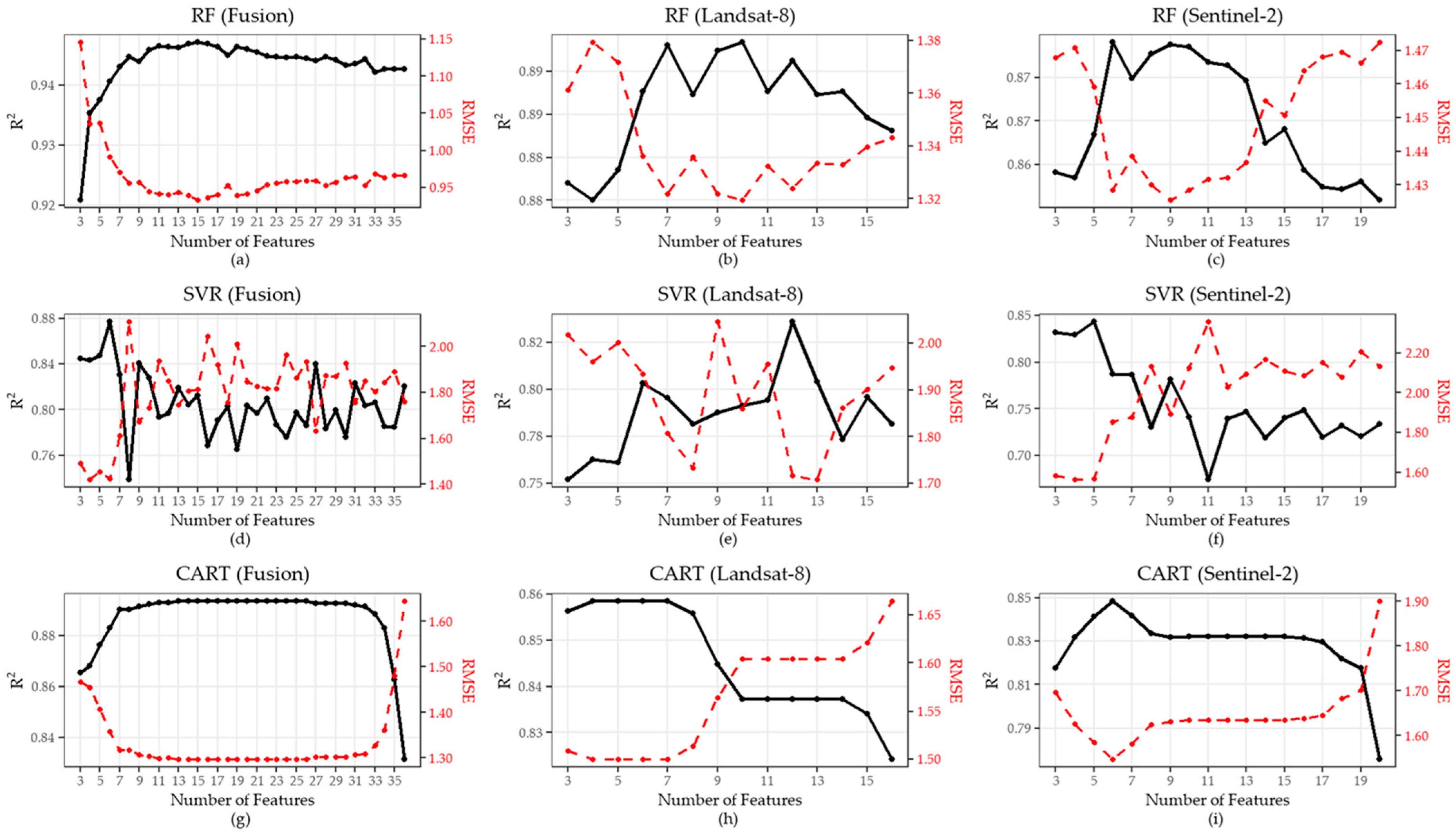
This step involved variable reduction to identify the most important predictors for rice yield prediction. The results are presented as line plots showing the relationships between the number of predictors and model performance (R2 and RMSE) for RF, CART, and SVR models. In each iteration, the least influential predictor was removed and the model was retrained with the remaining variables using 5 fold cross-validation. This process continued until only two predictors remained, after which the subset with the highest R2 and lowest RMSE was selected.
The results shown in Figure 10a–i indicated that the Random Forest model achieved steadily increasing R2 and consistently decreasing RMSE across all datasets. The Fusion dataset performed best (R2 ≈ 0.84, RMSE ≈ 0.19 with more than 10 predictors), followed by Landsat-8 (R2 = 0.80, RMSE = 0.21) and Sentinel-2 (R2 = 0.65, RMSE = 0.29). The SVR model showed similar trends, with Fusion again yielding the best results (R2 ≈ 0.83, RMSE ≈ 0.20), followed by Landsat-8 (R2 ≈ 0.72, RMSE ≈ 0.26) and Sentinel-2 (R2 ≈ 0.68, RMSE ≈ 0.31). In contrast, the CART model performed poorly and showed signs of underfitting, with Fusion reaching only R2 = 0.68 and Sentinel-2 obtaining the lowest values (R2 = 0.47, RMSE = 0.37).
In summary, the Fusion dataset consistently outperformed those derived from individual sensors; furthermore, Random Forest proved to be the most robust and accurate model, followed by SVR, while CART showed limited capability in handling the complex data.

3.1.3. Correlation Analysis of Rice Yield and Satellite Derived Variables

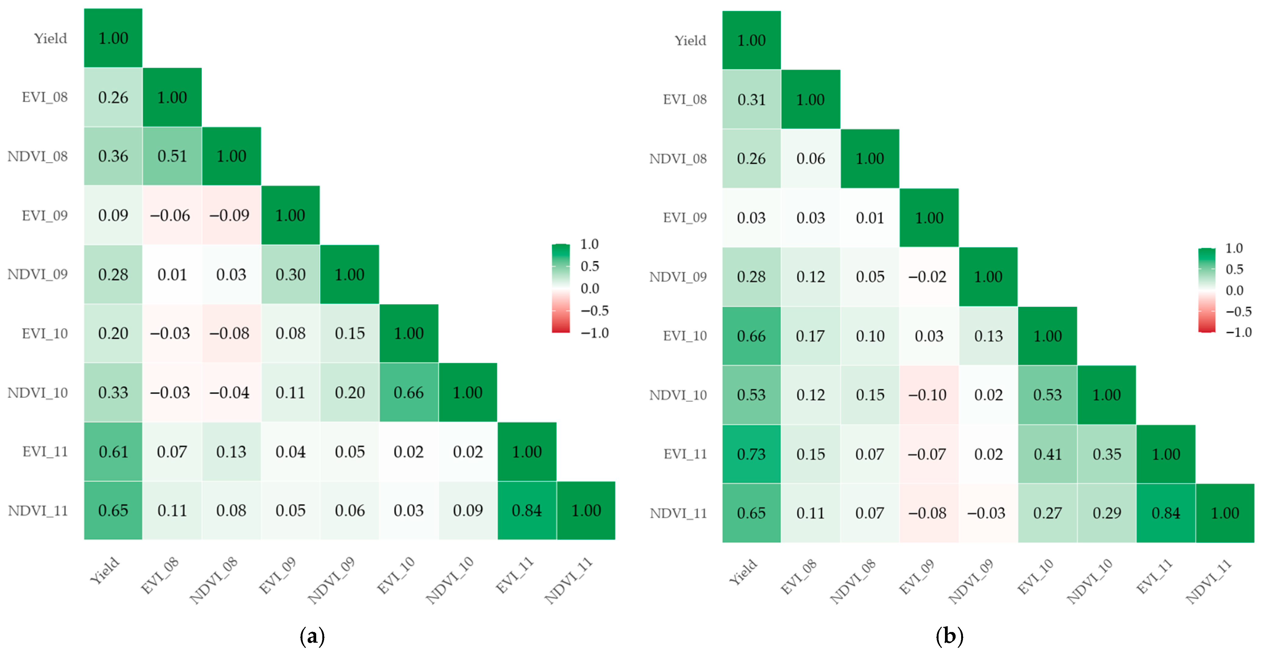
Pearson correlation analysis was performed to examine the relationships between rice yield and vegetation indices derived from Sentinel-2 and Landsat-8 data, as illustrated in Figure 11a,b. In these graphs, the suffixes denote the acquisition months, with 08 corresponding to August, 09 to September, 10 to October, and 11 to November. The correlation graphs were used not only to evaluate the direct associations between yield and vegetation indices, but also to identify and remove redundant or highly correlated features. For Sentinel-2, the strongest correlations were found in November with NDVI (r = 0.65) and EVI (r = 0.61), while earlier growth stages such as those in September and October showed weaker associations, particularly for EVI in September (r = 0.09). For Landsat-8, the highest correlation was observed for EVI in November (r = 0.73), followed by EVI in October (r = 0.66) and NDVI in November (r = 0.65). By contrast, indices from earlier months showed relatively low correlations, with the lowest value recorded for EVI in September (r = 0.03).
These results highlight that vegetation indices obtained during the reproductive to ripening stages (October–November) are the most reliable predictors of rice yield. The use of Pearson correlation graphs also enabled the elimination of redundant features, ensuring that only the most relevant indices were retained for model evaluation.
In addition to identifying the temporal patterns of yield–index relationships, the correlation analysis served as an essential diagnostic step prior to dimensionality reduction. It allowed us to evaluate multicollinearity among vegetation indices, understand the physical relevance of each predictor, and ensure that only meaningful and non-redundant variables were retained for subsequent machine learning modeling. This step strengthened both the transparency and interpretability of the variable selection process.

3.1.4. Final Feature Selection for Rice Yield Prediction

The final step of the variable reduction process was the selection of the top five predictors from each dataset (Fusion, Landsat-8, and Sentinel-2) for model evaluation and interpretation (Figure 12a–c). The results revealed that Random Forest, CART, and SVR models consistently identified vegetation indices derived during the reproductive to ripening stages (October–November) as the most influential predictors of rice yield. For Sentinel-2, NDVI and EVI from November were frequently selected across all models, confirming their strong predictive power during late growth stages. For Landsat-8 models, EVI in November, EVI in October, and NDVI in November were highlighted as key predictors, aligning with the observed high correlations between these indices and rice yield. In the Fusion dataset, a combination of indices from both sensors was selected, demonstrating the complementary contributions of Sentinel-2 and Landsat-8 to prediction accuracy.

3.1.5. Variable Importance Analysis and Model Interpretability for Rice Yield Prediction

After the final feature selection process, the importance of the remaining variables was evaluated and ranked using the Random Forest (RF) model, which showed the best performance based on the Fusion dataset. The results, presented in Figure 13, identify five key predictors derived from Landsat-8 and Sentinel-2 vegetation indices: Landsat-8 EVI_10 (100%), Sentinel-2 NDVI_10 (89.54%), Landsat-8 EVI_11 (72.44%), Sentinel-2 EVI_11 (38.11%), and Landsat-8 NDVI_09 (12.25%). Most of these indices correspond to the reproductive to ripening stages of rice growth (October–November), which exert the greatest influence on yield prediction. These predictors represent key physiological processes such as canopy greenness, chlorophyll concentration, and photosynthetic activity, all of which directly affect grain filling and yield potential.
Both the Enhanced Vegetation Index (EVI) and Normalized Difference Vegetation Index (NDVI) from Landsat-8 and Sentinel-2 exhibited high sensitivity to variations in canopy vigor and biomass accumulation, effectively reflecting the physiological condition and stress responses of the crop. The strong importance of Landsat-8 EVI (October) and Sentinel-2 NDVI (October) indicates that spectral information captured during the reproductive stage provides the most reliable yield predictors, corresponding to peak panicle development and assimilate translocation. Meanwhile, EVI (November) from both sensors captured physiological changes during the ripening phase—such as chlorophyll degradation and reduced photosynthetic activity—whereas Landsat-8 NDVI (September) represented early vegetative establishment, contributing contextual information despite its lower importance. The physiological relevance of these variables is supported by their strong contribution to the model’s performance. The dominance of EVI and NDVI during October–November corresponds to the period of maximum leaf area index (LAI) and peak photosynthetic rate reported in rice phenology studies, confirming that canopy greenness and chlorophyll activity are the main factors determining yield formation. These findings indicate that the spectral–physiological relationship captured by EVI and NDVI effectively converts canopy dynamics into quantitative variations in rice yield within the RF model. Integrating Sentinel-2′s high spectral–spatial resolution with Landsat-8’s temporal consistency enhanced cross-sensor complementarity, enabling the RF model to better capture physiological variations and growth dynamics, thereby improving interpretability and predictive accuracy in rice yield modeling.
In summary, vegetation indices derived from the late growing season, particularly EVI and NDVI from October to November, serve as critical indicators for rice yield estimation. These findings provide a robust foundation for yield forecasting, precision crop management, and advanced applications of precision agriculture across tropical rice-growing regions.

3.1.6. Model Performance for Rice Yield Prediction

Three satellite derived datasets were used in this study: Dataset 1 from Landsat-8, Dataset 2 from Sentinel-2, and Dataset 3 as a fusion of Landsat-8 and Sentinel-2 data. The performance of three machine learning models—RF, CART, and SVR—was evaluated based on the coefficient of determination (R2) and Root Mean Square Error (RMSE) values.
The RF model consistently outperformed CART and SVR across all datasets. On Dataset 1, RF achieved a training R2 of 0.96 with an RMSE of 0.10, while the validation results remained high with an R2 of 0.82 and an RMSE of 0.21. CART produced weaker validation results, with an R2 of 0.68 and an RMSE of 0.28; while SVR showed similar performance with an R2 of 0.65 and an RMSE of 0.37. Dataset 2 was more challenging: RF still performed best, with a validation R2 of 0.64 and RMSE of 0.30. CART achieved an R2 of 0.50 and RMSE of 0.35, while SVR reached an R2 of 0.60 and RMSE of 0.42. The lower performance metric values suggest greater variability or noise in Dataset 2. Dataset 3 produced the highest accuracy: RF again led with a training R2 of 0.97 and RMSE of 0.09, and a validation R2 of 0.86 and RMSE of 0.19. SVR performed well, with a validation R2 of 0.72 and RMSE of 0.33, thus surpassing CART with an R2 of 0.70 and RMSE of 0.26. The performance metrics are detailed in Table 4.
The spatial rice yield prediction maps for all models (Figure 14a–i) clearly demonstrate the superior performance of the RF model, particularly on Dataset 3, as the RF-generated maps exhibit smoother and more consistent spatial patterns across Northeastern Thailand, while the outputs from CART and SVR show greater noise and variability. These spatial results highlight RF’s strong ability to generalize under diverse agricultural conditions, especially when utilizing multi-source spectral indices.
Due to its superior predictive performance, the RF algorithm was selected for the diagnostic analysis and robustness evaluation. For this rice yield model, residual plots, histograms, and Q–Q plots indicated that the residuals were approximately normally distributed, with no bias or heteroscedasticity. Cross-validation and bootstrapping confirmed its consistent performance (R2 = 0.829–0.845, RMSE = 0.208–0.221), while sensitivity tests indicated minimal variation (ΔR2 ≤ 0.012, ΔRMSE ≤ 0.010), demonstrating the model’s stability and robustness in rice yield prediction. Although the rice yield models demonstrated high accuracy, some residual errors persisted, mainly due to satellite image noise, cloud contamination, and temporal mismatches between imagery and field data. These errors reflect the complex nature of rice yield formation, influenced by factors such as soil fertility, moisture availability, irrigation and fertilizer management, and climatic variability. Future research integrating multi temporal datasets and advanced image processing techniques could further enhance the accuracy and reliability of rice yield prediction. Overall, the findings confirm that RF, when using NDVI and EVI from Sentinel-2 and Landsat-8, delivers the most accurate and spatially reliable rice yield predictions. This integrated method shows strong potential for precision agriculture, yield forecasting, and sustainable management in Thailand and similar regions.

3.2. Soil Salinity Estimation Models

3.2.1. Variable Reduction Results for Soil Salinity Models

The same variable reduction approach described in Section 3.1.2 was applied to the soil salinity models to identify the most important predictors. The corresponding results are presented as line plots depicting the variation of R2 and RMSE for the RF, CART, and SVR models. As shown in Figure 15a–i, model performance improved rapidly during the early stages of variable selection, where weak predictors were eliminated. The RF model achieved the highest accuracy on the Fusion dataset, with R2 values stabilizing around 0.93 and RMSE decreasing to approximately 0.95 once 10–12 features were retained. Similarly, SVR demonstrated strong performance on the Fusion data, reaching an R2 of 0.90 and RMSE of 1.10 before a slight decline was observed when additional features were included. For the single sensor datasets, Landsat-8 generally outperformed Sentinel-2 across all three algorithms. The RF model using Landsat-8 achieved a maximum R2 of 0.876 and RMSE of 1.34, while Sentinel-2 RF stabilized at an R2 of 0.838 and RMSE of 1.42. SVR also showed improved performance with Landsat-8, reaching an R2 of 0.82, compared to an R2 of 0.80 with Sentinel-2. The CART models achieved lower performance overall but still benefited from reduced variable sets, with their accuracy stabilizing once 4–6 features were retained.
In summary, variable reduction enhanced efficiency and prevented overfitting, with Fusion yielding the best results, followed by Landsat-8, while Sentinel-2 alone showed lower accuracy.

3.2.2. Correlation Analysis of EC and Satellite Derived Variables

Pearson correlation analysis was conducted to evaluate the relationships between soil salinity, measured as electrical conductivity (EC), and spectral information derived from Sentinel-2 and Landsat-8 imagery. Figure 16 and Figure 17 show the correlations between EC, spectral bands, and vegetation and salinity indices, revealing clear and consistent patterns that emphasize the complementary roles of vegetation and salinity indices in detecting soil salinity stress.
For Landsat-8 data, EC exhibited strong negative correlations with vegetation indices such as NDVI (r = −0.68), GNDVI (r = −0.68), and EVI (r = −0.65), suggesting that higher soil salinity reduces vegetation vigor, leading to lower index values and reflecting the indirect effects of salt stress on plant health. Conversely, the salinity indices showed positive correlations, with SI1 (r = 0.76), SI2 (r = 0.52), and SI3 (r = 0.51) emerging as particularly responsive to salinity variations. Among the spectral bands, Band 2 (blue; r = 0.55) and Band 3 (green; r = 0.32) showed moderate positive correlations with EC, indicating their sensitivity to surface reflectance changes caused by salt crusts and soil brightness.
For Sentinel-2 data, the correlation structure closely mirrored that of Landsat-8, but with enhanced sensitivity in certain spectral bands. EC displayed significant negative correlations with NDVI (r = −0.68), GNDVI (r = −0.70), and EVI (r = −0.26), reinforcing the evidence that vegetation indices effectively capture the stress response of crops to salinity. The salinity indices again showed strong positive correlations: SI1 (r = 0.70), SI2 (r = 0.72), and SI3 (r = 0.65). Importantly, Sentinel-2’s shortwave infrared (SWIR) bands were particularly effective, with Band 11 (SWIR1; r = 0.78) and Band 12 (SWIR2; r = 0.26) demonstrating significant correlations. This finding highlights the critical role of SWIR wavelengths in detecting soil salinity, as they are highly responsive to soil moisture and mineral absorption features.
Overall, these correlation analyses highlight two complementary mechanisms for soil salinity detection. On one hand, indirect indicators such as vegetation indices (NDVI, GNDVI, and EVI) capture the physiological stress caused by salinity, reflected in reduced canopy vigor and greenness; on the other hand, direct indicators including salinity indices (SI1–SI3) and SWIR bands (B11, B12) provide spectral evidence for the accumulation of salt in the soil itself. In addition to interpreting the spectral response of salinity stress, the correlation analysis also served as a diagnostic step prior to dimensionality reduction. It helped identify redundant or highly collinear predictors and ensured that only meaningful and non-overlapping variables were retained for subsequent model training.

3.2.3. Final Feature Selection for Soil Salinity Models

Feature selection allowed for identification of the most influential predictors for estimating soil salinity across the three datasets—Fusion, Landsat-8, and Sentinel-2—when using RF, CART, and SVR models. For the Fusion dataset, salinity indices SI1–SI5 and vegetation indices such as NDVI, GNDVI, and NDWI were consistently ranked as highly important, along with visible spectral bands B2 to B4. For the Landsat-8 dataset, vegetation indices including NDVI, GNDVI, and EVI were emphasized alongside salinity indices SI2, SI4, and SI5, as well as the green band (B3), highlighting their roles in capturing soil salinity signals. For the Sentinel-2 dataset, the salinity indices SI1–SI5 emerged as the dominant predictors, supported by the blue and green spectral bands (B2–B4), reflecting the higher sensitivity of Sentinel-2 in detecting soil salinity conditions. A detailed summary of the final selected features is presented in Figure 18a–c.

3.2.4. Variable Importance Analysis and Model Interpretability for Soil Salinity

After the final feature selection process, variable importance was evaluated and ranked using the Random Forest (RF) model developed from the Fusion dataset, as illustrated in Figure 19. The results identified the five most influential predictors contributing to soil salinity prediction accuracy: Sentinel-2_SI3 (100%), Sentinel-2_B2 (91.83%), Sentinel-2_B3 (71.75%), Sentinel-2_GNDVI (68.22%), and Landsat-8_NDWI (29.29%).
The Sentinel-2_SI3 (100%), a salinity index derived from Sentinel-2 spectral bands, was the strongest driver of model performance. It effectively detected saline soils through spectral reflectance patterns associated with surface salt crusts and soil albedo, allowing clear differentiation between saline and non-saline areas even under varying soil moisture conditions. The Sentinel-2_B2 (91.83%) and Sentinel-2_B3 (71.75%) bands, corresponding to the blue and green regions of the spectrum, were also highly influential due to their sensitivity to surface brightness, salt deposits, and fine salt particles—enhancing the model’s ability to capture direct spectral cues of salinity. In contrast, Sentinel-2_GNDVI (68.22%) captured vegetation stress induced by saline conditions, reflected by reductions in chlorophyll content, canopy greenness, and biomass. This index provided an indirect indicator of soil salinity effects on plant health. Meanwhile, Landsat-8_NDWI (29.29%) contributed complementary information on soil moisture variability, helping to distinguish between wet saline soils (often following rainfall or irrigation) and dry saline areas characterized by surface salt crystallization.
Overall, the integration of both sensors (cross-sensor complementarity) enabled the RF model to simultaneously capture direct spectral salinity signals from Sentinel-2 and contextual soil moisture information from Landsat-8, thereby improving both interpretability and accuracy. These findings reveal the interconnected relationships among spectral processes, soil surface characteristics, and vegetation physiological responses, offering valuable insights for regional-scale soil salinity mapping and monitoring under diverse environmental conditions.

3.2.5. Model Performance for Soil Salinity Estimation

This study assessed the performance of regression models constructed using three machine learning algorithms—RF, CART, and SVR—in mapping the spatial distribution of soil salinity. Each model was systematically configured with optimized parameters to enhance their predictive accuracy.
The modeling process commenced with the identification of relevant environmental covariates and the analysis of correlations among various spectral band combinations. The selection of variables was based on their statistical relationships with the field measured soil electrical conductivity (EC). Three distinct datasets were employed for model development: one derived from Landsat-8 imagery, one from Sentinel-2 imagery, and a third integrating features from both sensors.
Initially, 36 environmental variables were evaluated and subsequently refined through variable reduction. Following this reduction and visual evaluation of the soil salinity maps, only the indices and spectral bands showing strong correlations with soil electrical conductivity (EC) were selected for use in each specific dataset. In Dataset 1 (from Landsat-8), the selected variables were SI2, SI3, SI4, B3 (green band), and NDWI. Those for dataset 2 (from Sentinel-2) included SI1, SI3, SI4, B2 (blue band), and NDWI. For Dataset 3 (combining both Landsat-8 and Sentinel-2), SI1, SI3, and SI4 were taken from Sentinel-2, while SI1 and NDWI were used from Landsat-8. The selection of these indices and bands was guided by their high correlation with EC. Although NDWI from Landsat-8 showed the lowest correlation, it was included due to its proven effectiveness in detecting moisture in vegetation and soil surfaces. In highly saline areas, reduced moisture content leads to lower NDWI values, making it a valuable indirect indicator of soil salinity.
As summarized in Table 5, the model performance assessment results showed that, across all datasets, the Random Forest model consistently outperformed the Classification and Regression Trees and Support Vector Regression models in terms of predictive accuracy and stability. For Dataset 1 (based on Landsat-8), Random Forest achieved an R2 of 0.97 with an RMSE of 0.62 during training and an R2 of 0.83 with an RMSE of 1.36 during validation. Classification and Regression Trees and Support Vector Regression demonstrated lower accuracy, yielding validation R2 values of 0.78 and 0.77, respectively. In Dataset 2 (based on Sentinel-2), Random Forest again achieved the highest performance, with an R2 of 0.96 and RMSE of 0.65 during training and an R2 of 0.81 and RMSE of 1.46 during validation. Classification and Regression Trees and Support Vector Regression performed comparatively worse, with validation R2 values of 0.76 and 0.76, respectively. The highest accuracy was observed in Dataset 3 (based on the fusion of Landsat-8 and Sentinel-2), where Random Forest attained an R2 of 0.98 and RMSE of 0.38 during training and an R2 of 0.93 and RMSE of 0.87 during validation. The performance metrics of the Classification and Regression Trees and Support Vector Regression models also improved under the fusion dataset, with validation R2 values of 0.85 and 0.81, although still outperformed by Random Forest.
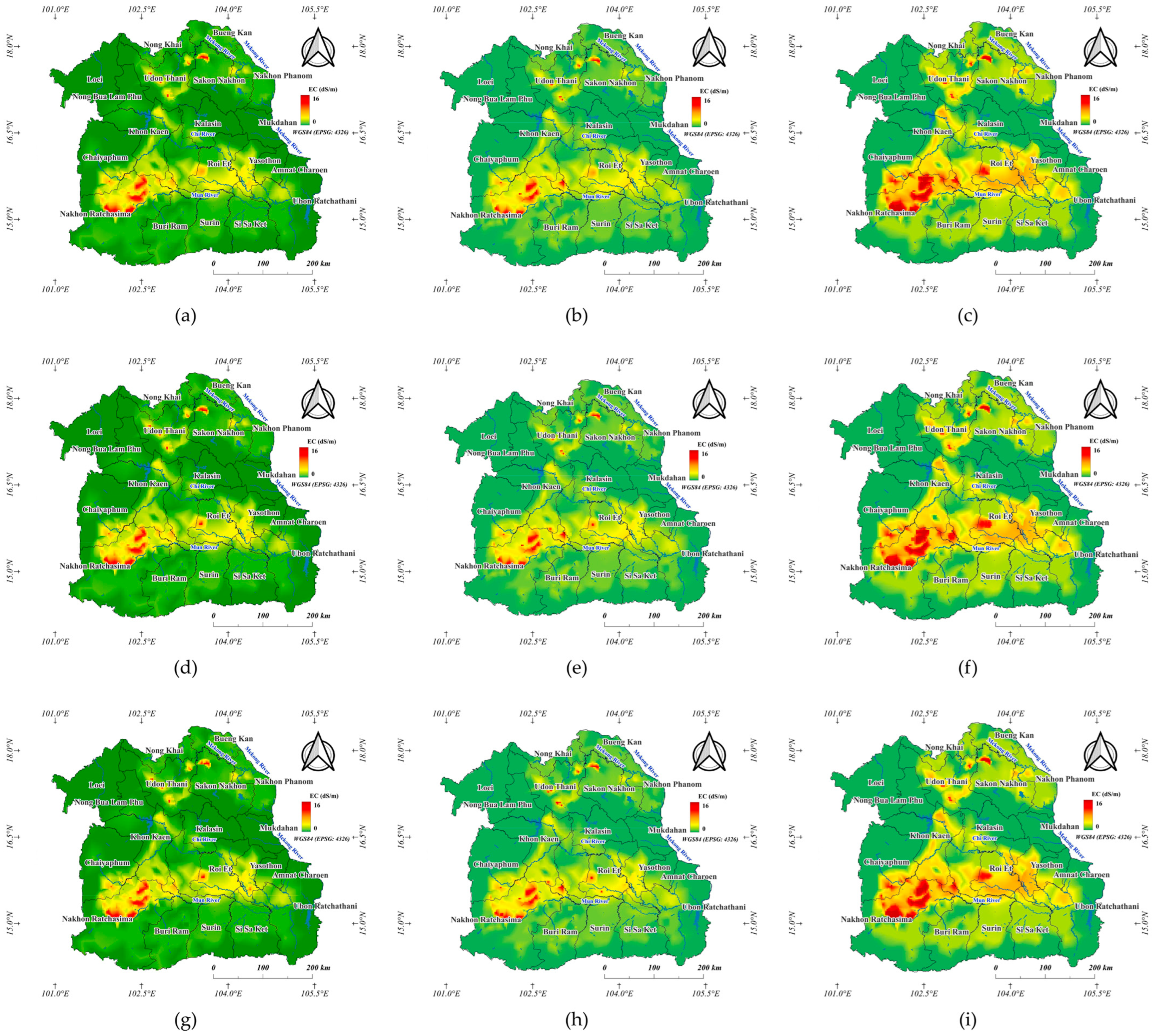
The model-generated maps are shown in Figure 20a–i, with the spatial distribution results indicating that all models captured the variations in salinity across Northeastern Thailand. The RF algorithm was selected for Soil Electrical Conductivity (EC) modeling due to its superior predictive performance (in terms of R2 and RMSE) compared with the other models. Diagnostic analysis indicated that its residuals were approximately normally distributed, with no bias or signs of heteroscedasticity. Robustness tests, including cross-validation and bootstrapping, confirmed its stable performance, with R2 = 0.884–0.902 and RMSE = 0.243–0.271. Parameter and outlier sensitivity analyses indicated minimal variation (ΔR2 ≤ 0.008, ΔRMSE ≤ 0.008), demonstrating the model’s high stability, reproducibility, and robustness in estimating soil electrical conductivity. Although the soil salinity models demonstrated high predictive accuracy, certain residual errors persisted, primarily due to satellite image noise, cloud contamination, and temporal mismatches between remote sensing data acquisition and field observations. Such discrepancies may also reflect the inherent complexity of soil salinity dynamics, which are governed by interacting factors including soil texture, moisture variability, evapotranspiration, and irrigation regimes that fluctuate across spatial and temporal scales. Future studies incorporating advanced cloud removal algorithms and multi temporal datasets are expected to further enhance the robustness, precision, and reliability of soil salinity estimation. Overall, it was found that the fusion of Sentinel-2 and Landsat imagery with machine learning algorithms particularly RF can significantly improve soil salinity estimation, thus supporting precision agriculture applications.

3.3. Correlation Between Rice Yield and Soil Electrical Conductivity (EC)

The spatial relationship between soil salinity and rice yield during the seedling stage was examined using 5000 randomly selected points derived from the soil electrical conductivity (EC) model for June–July, in order to analyze the spatial variability of soil salinity and its impact on rice yield. Rice yield values at the corresponding locations were extracted from the rice yield prediction model to assess the relationship between soil salinity and rice productivity. The seedling stage is widely recognized as the period in which the plants are most sensitive to soil salinity stress [11], as elevated salinity levels can significantly reduce seedling survival and tillering capacity, ultimately leading to lower yields.
The scatter plot shown in Figure 21 depicts a clear negative relationship between EC and rice yield, with a polynomial trend line indicating a decrease in yield as EC increases. The analysis revealed a statistically significant negative correlation, with an R-squared value of 0.71, suggesting that approximately 71% of the variation in rice yield can be explained by soil EC levels during the seedling stage. The yield data exhibit moderate variability, with an average of 2.82 t ha−1and a standard deviation of 0.60, while EC values show a broader range of variation (mean = 5.98 dS/m, standard deviation = 3.76), as summarized in Table 6. These patterns highlight that lower EC zones exhibit more yield variability, whereas higher EC zones consistently correspond to reduced rice productivity. Overall, the findings emphasize the detrimental impact of elevated soil salinity on rice production potential, particularly during the early growth stages.

4. Discussion

4.1. Comparative Evaluation of Machine Learning Models for Rice Yield Prediction

Comparative analysis of the three satellite derived datasets demonstrated that the RF model achieved the highest predictive accuracy for rice yield forecasting. RF consistently outperformed CART and SVR in both the training and validation phases, especially on the fused Landsat-8 and Sentinel-2 dataset (R2 = 0.86, RMSE = 0.19). This study highlights the potential of ensemble learning methods in modeling complex and nonlinear relationships between spectral indices and rice yield. In practical applications, the Random Forest (RF) model enables the generation of near-real-time spatial yield maps that support fertilizer management, irrigation scheduling, and crop insurance assessment. These spatial datasets serve as valuable tools for enhancing regional agricultural management under climatic and resource constraints.
The performance differences among datasets also provides important insights. Dataset 1 (Landsat-8) delivered reliable results (validation R2 = 0.82, RMSE = 0.21), whereas Dataset 2 (Sentinel-2) produced comparatively lower accuracy (validation R2 = 0.64, RMSE = 0.30). The fusion dataset mitigated both limitations, achieving a balance between spatial detail and temporal consistency. Practically, this fusion ensures monitoring continuity during cloudy or monsoon seasons, which is particularly advantageous for tropical regions such as Thailand. This outcome reflects the greater sensitivity of Sentinel-2 to cloud contamination and seasonal variability, despite its higher spatial resolution. In this study, most Sentinel-2 scenes were heavily cloud-covered, resulting in only a small portion of usable imagery and reduced temporal reliability consistent with the findings of Useya and Chen [67] who reported that cloud cover significantly limits the data availability of Sentinel-2, whereas Landsat imagery offers more consistent and temporally stable observations. Similar findings have been reported by Son et al. [18,19], who observed that MODIS and Sentinel-2 datasets yielded variable accuracies depending on temporal coverage and atmospheric conditions. In contrast, the Fusion dataset (Dataset 3) provided a balanced advantage, mitigating the temporal limitations of Landsat-8 and the noise effects of Sentinel-2. This aligns with the works of Zhang et al. [22] and Dhillon et al. [23], who demonstrated that multi-sensor integration enhances yield predictions by leveraging the complementary strengths of the different sensors. The accuracy gains obtained through fusion also underscore the importance of spatio-temporal complementarity in satellite data. While Landsat-8 offers long term continuity and consistent radiometric calibration, Sentinel-2 provides finer spatial detail but is more susceptible to missing observations due to cloud cover. By combining these datasets, the fusion approach improves temporal density and reduces uncertainty, resulting in more robust performance among the tested scenarios. These findings parallel the conclusions of Meng et al. [24], who found that fused MODIS–Landsat NDVI reconstructions significantly improved predictive accuracy compared to single sensor approaches.
When compared with the existing literature, the results of this research are comparable to or exceed previously reported accuracies. For instance, RF applied to MODIS NDVI time series achieved RMSE values between 5.6 and 11.8% in the study of Son et al. [18], while the present study achieved an RMSE of 0.19 t ha−1 in the fusion dataset. Similarly, Chaiyana et al. [21] demonstrated that, when integrating MODIS based vegetation indices with climatic and drought indices, the resulting XGBoost model achieved R2 = 0.95. Although the absolute R2 values differ, the relative improvement observed in the present study through fusion and ML confirms the broader consensus that integrated data sources combined with advanced ML models deliver superior yield predictions. Notably, the workflow relies solely on freely available optical imagery, underscoring its cost-effectiveness and scalability for data-constrained regions. Accordingly, the study provides actionable guidance for establishing national or provincial yield-monitoring systems based on open-access EO data.
The superior accuracy of the RF model compared to SVR and CART is attributed to its ensemble learning structure, which combines the outputs of multiple decision trees through bootstrap sampling and random feature selection. This enables RF to effectively capture complex nonlinear relationships between vegetation indices and rice yield while minimizing overfitting. Moreover, RF is less sensitive to parameter tuning and can efficiently handle multi collinearity and high noise spectral data across multiple bands [17,18,68,69]. In practice, this stability enables the RF model to consistently predict rice yield across diverse agricultural environments. The ability of RF to integrate Landsat-8 and Sentinel-2 fusion data enhances both spatial continuity and predictive accuracy, confirming its suitability for precision agriculture applications and regional scale yield monitoring. These results are consistent with previous studies such as those of Son et al. [18] and Choudhary et al. [17], who demonstrated that RF and other ensemble methods perform highly effectively in agricultural yield prediction.
Spectral indices such as NDVI and EVI are physiologically linked to key processes governing rice growth and yield formation. Higher NDVI and EVI values during the vegetative and reproductive stages indicate vigorous canopy development, higher chlorophyll content, and greater leaf area index (LAI) [18,19], all of which enhance photosynthetic efficiency and biomass accumulation. These physiological relationships were clearly reflected in the Random Forest (RF) model results, which identified five major predictors—Landsat-8 EVI (October, 100%), Sentinel-2 NDVI (October, 89.54%), Landsat-8 EVI (November, 72.44%), Sentinel-2 EVI (November, 38.11%), and Landsat-8 NDVI (September, 12.25%). These indices correspond to the reproductive and ripening stages (October–November), when chlorophyll activity and canopy vigor peak, directly influencing grain filling and yield potential. Under saline stress, sodium and chloride accumulation in the root zone causes osmotic imbalance and ion toxicity, reducing chlorophyll synthesis and photosynthetic activity [70,71], which manifests as lower NIR reflectance and reduced NDVI/EVI values. The RF model effectively captured these spectral–physiological linkages, demonstrating its capability to interpret physiological responses and improve yield prediction accuracy through multi-sensor data fusion.
Under saline conditions, however, excessive sodium and chloride ions accumulate in the root zone, causing osmotic stress and ion toxicity that disrupt water uptake and nutrient balance. This leads to reduced chlorophyll synthesis, lower stomatal conductance, and early leaf senescence—physiological effects that diminish photosynthetic efficiency and total biomass [72,73]. This stress responses manifest as reduced near-infrared (NIR) reflectance and lower NDVI/EVI values, which are effectively captured by the RF model. Thus, the strong correlations identified between vegetation indices and yield represent not only empirical statistical relationships but also the physiological mechanisms underlying salinity-induced yield reduction.
The ensemble architecture of the Random Forest (RF) model enables the integration of signals from multiple spectral regions (red, green, and NIR) and effectively captures nonlinear relationships between plant stress and spectral reflectance [28,29]. Through this process, the model implicitly learns the spectral signatures associated with physiological resilience and stress tolerance in rice, accounting for its superior robustness and biological interpretability. This mechanistic linkage bridges plant physiological responses with model performance, strengthening confidence in the application of multi-sensor fusion and machine learning frameworks for yield estimation under variable environmental and salinity conditions.
From an operational standpoint, the integration of multi-sensor fusion and RF modeling establishes a scalable, transferable framework that can be adopted by agricultural agencies, crop-insurance providers, and water-resource managers. It facilitates proactive yield forecasting, optimizes irrigation and input management, and supports risk-based insurance planning. Moreover, its capability to provide near-real-time spatial intelligence contributes to climate adaptation strategies and food-security monitoring across local and regional scales, thereby promoting precision agriculture and agricultural sustainability in data-limited environments such as Southeast Asia.

4.2. Comparative Assessment of Machine Learning Models for Soil Salinity Estimation

The findings of this study clearly demonstrate the superiority of RF over CART and SVR in soil salinity estimation. RF consistently achieved higher R2 and lower RMSE values across all datasets, with its performance further enhanced when applied to the fused Landsat-8 and Sentinel-2 dataset. This observation aligns with previous research, such as that of Haq et al. [32], who reported RF as the best performing algorithm (R2 = 0.94, RMSE = 1.89 dS/m) when compared with other regressors using Landsat-8 data, while Aksoy et al. [31] and Bandak et al. [34] have also emphasized the robustness of tree based approaches for salinity mapping.
The Random Forest (RF) model developed using the fused Landsat-8 and Sentinel-2 dataset identified five major predictors contributing to soil salinity estimation accuracy: Sentinel-2_SI3 (100%), Sentinel-2_B2 (91.83%), Sentinel-2_B3 (71.75%), Sentinel-2_GNDVI (68.22%), and Landsat-8_NDWI (29.29%). Among these, Sentinel-2_SI3 was the most influential variable, effectively detecting saline soils through spectral reflectance associated with surface salt crusts and soil brightness, consistent with previous studies [30,31,32,34], which emphasized the capability of salinity indices (SI series) in identifying salt-affected areas using Sentinel-2 and Landsat-8 data. The blue (B2) and green (B3) bands were also highly sensitive to salt deposits and surface albedo, supporting the findings of [74,75], who reported that these spectral regions are particularly sensitive to salt deposits.
Meanwhile, Sentinel-2_GNDVI acted as an indirect indicator of vegetation stress under saline conditions, such as chlorophyll reduction and decreased canopy vigor, consistent with [76,77]. Additionally, Landsat-8_NDWI provided complementary information on soil-moisture variability, helping to distinguish between wet saline soils and dry crystallized salt surfaces. This agrees with Aksoy et al. [31] and Ma and Tashpolat [33], who highlighted the importance of moisture-related indices (e.g., NDWI) for enhancing salinity detection in arid environments. Overall, the integration of multi-sensor satellite data substantially improved the model’s capability to capture both direct and indirect salinity signals, demonstrating the robustness of the RF model in linking spectral characteristics, soil-surface properties, and vegetation responses for accurate soil-salinity mapping across diverse tropical environments.
The integration of multi-sensor data improved the model’s capacity to capture both direct and indirect salinity signals, demonstrating the effectiveness of RF in linking spectral characteristics, soil surface conditions, and vegetation responses for accurate soil salinity mapping in diverse tropical environments.
The RF model outperformed CART and SVR in predicting soil salinity by effectively capturing nonlinear relationships and managing complex multi-source spectral data. The random variable and sample selection processes in RF reduce overfitting and multi collinearity, which are common in Landsat-8 and Sentinel-2 datasets [78,79]. RF also identified key predictors, consistent with Aksoy et al. [31] and Wang et al. [80], demonstrating its ability to detect both direct salinity signals and vegetation stress. In contrast, CART and SVR showed weaker performance. These results confirm that RF is highly suitable for generating high resolution and accurate soil salinity maps, which are valuable for precision agriculture and soil restoration planning [31].
The fused dataset (Landsat-8 + Sentinel-2) achieved the highest accuracy (R2 = 0.93; RMSE = 0.87 in validation with RF), confirming that multi-source integration provides complementary spectral information and enhances model generalizability. This finding supports the works of Wang et al. [35], who showed that integrating optical, radar, and thermal data significantly improved salinity mapping (R2 = 0.75), and Kholdorov et al. [36], who demonstrated that fusing Sentinel-2 and Landsat-8 with feature selection produced highly accurate predictions (R2 = 0.96; RMSE ≈ 4.1). At a global scale, Wang et al. [37] further highlighted the benefits of multi-source integration by successfully developing a 10 m resolution global soil salinity model using Sentinel-1/2, climate, and terrain data. While the single source datasets (Landsat-8, Sentinel-2) produced reasonable results, their fusion consistently outperformed individual sensors.
Together with the present findings, these studies highlight that multi-sensor fusion is not only beneficial but often necessary for reliable soil salinity mapping in heterogeneous landscapes. This outcome reflects the greater sensitivity of Sentinel-2 to extensive cloud cover and seasonal variability, despite its higher spatial resolution. In this study, most Sentinel-2 scenes had much cloud cover, resulting in only a small proportion of usable imagery and reduced temporal reliability, consistent with the findings of Useya and Chen [67], who reported that cloud cover substantially restricts the data availability of Sentinel-2, whereas Landsat imagery provides more consistent and temporally stable observations.
From a physiological standpoint, the spectral predictors identified by the RF model are directly linked to the mechanisms governing rice response under salt stress. High salinity leads to excessive accumulation of sodium (Na+) and chloride (Cl) ions in the root zone, causing osmotic imbalance, ion toxicity, and impaired water uptake. These processes reduce chlorophyll synthesis and photosynthetic efficiency, resulting in lower canopy vigor and decreased near-infrared (NIR) reflectance [76,81]. Consequently, vegetation indices such as GNDVI and NDWI decline, reflecting stress-induced reductions in leaf water content and greenness [82,83]. Conversely, the SI3 index, which integrates visible and shortwave spectral information, captures surface salt crusts and soil brightness caused by salt efflorescence [30,31,32,34]. The strong performance of these variables in the RF model thus reflects its ability to physiologically discriminate between direct soil salinity signals and vegetation responses. This mechanistic linkage provides empirical support for the model’s predictive behavior and strengthens confidence in its general applicability across varying soil–plant conditions.
From a practical perspective, the RF-based fusion approach provides a scalable and operational framework for salinity monitoring, land rehabilitation, and precision irrigation management. High-resolution salinity maps derived from this model can help farmers and land managers identify salinized zones, optimize soil amendment practices, and prevent yield losses in vulnerable areas. Local authorities can use these outputs as decision-support layers to prioritize land reclamation projects, manage irrigation water more efficiently, and design sustainable salinity control programs in semi-arid and tropical regions such as Northeast Thailand. Moreover, the workflow relies entirely on freely available satellite imagery, making it cost-effective and easily replicable in data-limited regions.
Although EC estimation was conducted at a broad regional scale, the approach does not overlook the influence of land-cover variation. The spectral predictors used in the model inherently capture vegetation and soil-surface characteristics, enabling the detection of salinity signals even across heterogeneous land-cover types. This is supported by Shrestha [84], who demonstrated that remote sensing could detect salinity both directly from bare soil and indirectly through vegetation responses, with spectral and chemical soil properties exhibiting strong relationships with measured EC. These findings indicate that the spectral variables employed in the model already incorporate essential land-cover information, contributing to the reliability of regional EC mapping. Nevertheless, future studies may benefit from explicitly integrating land-cover stratification to further improve the precision of salinity patterns across different land-cover classes.
Despite the promising results, some limitations remain. Cloud contamination in Sentinel-2 imagery reduced data quality, suggesting the need for improved cloud masking and temporal interpolation techniques. Optical data alone may not capture the full complexity of soil salinity; integrating radar (Sentinel-1) and thermal (Landsat TIRS) information could enhance prediction accuracy. As traditional models (RF, CART, SVR) have limited capacity to represent complex spatio-temporal dynamics, future studies should explore deep learning approaches such as CNNs and LSTMs, as demonstrated by Liu et al. [38]. The present study focused on Northeast Thailand, a region with distinct soil and environmental conditions; therefore, extending this approach to other agro-ecological zones would further test the model’s generalizability and policy relevance.

4.3. Relationship Between Soil Salinity and Rice Yield

This study reveals a statistically significant and strongly negative correlation between soil electrical conductivity (EC) during the rice seedling stage and grain yield; in other words, rice yield consistently decreases as soil salinity increases, highlighting salinity as a major factor constraining rice production. This finding is consistent with widely recognized physiological mechanisms, including osmotic stress, ion toxicity, and nutrient imbalances, all of which impair water uptake, reduce photosynthetic efficiency, and hinder biomass accumulation in rice plants [3]. The results also align with regional studies, particularly those conducted in Northeast Thailand such as Khon Kaen Province, where soil salinity has been shown to significantly impact rice yields. The effect becomes even more pronounced under drought conditions, when salinity levels tend to increase sharply [85]. Notably, this study confirms that rice is particularly sensitive to soil salinity during the seedling stage, when the root system is not yet fully developed. Stress at this stage can have long lasting impacts on growth and, consequently, yield a finding that is consistent with earlier work [10,11].
The best performing model, Random Forest (RF) using the Fusion dataset, revealed a strong negative relationship between soil electrical conductivity (EC) and rice yield. Yield remained high (around 3 t ha−1) when EC was below 5 dS m−1 but declined sharply within the range of 1.9–3.0 dS m−1, marking the onset of osmotic stress caused by increasing salinity. This stress reduces the soil osmotic potential, limits water uptake, and suppresses photosynthesis and growth, reflecting the high sensitivity of rice to even slight increases in salinity, consistent with previous findings [6].
When EC exceeded 5 dS m−1, yield continued to decrease, indicating the transition to the ion toxicity phase, driven by the accumulation of Na+ and Cl in roots and leaves. This accumulation damages cell membranes, disrupts metabolism, and lowers the K+/Na+ ratio, thereby reducing the uptake of essential nutrients (K+, N, and P) and photosynthetic activity. Such conditions correspond to cumulative salinity stress, which may result in tissue degradation and inhibition of panicle and grain formation, as supported by previous studies [86,87,88,89]. When EC exceeded 15 dS m−1, rice yield remained below 1.5 t ha−1, representing a physiological threshold beyond which rice can no longer tolerate salinity stress. Excessive salt accumulation at this level leads to severe cellular damage, ion imbalance, and metabolic failure, ultimately causing chlorophyll degradation, photosynthetic inhibition, and root system collapse. This terminal response corresponds to the final stage of salinity stress, consistent with Zeng and Shannon [11], who reported that rice growth and productivity cease once soil salinity surpasses this critical limit. Overall, the models confirmed the negative EC–yield relationship and identified key physiological thresholds (1.9–3, 5, and >15 dS m−1), providing a coherent link between quantitative modeling and the physiological mechanisms underlying rice salt tolerance.
These empirically derived breakpoints provide a valuable decision-support framework for managing salinity in irrigated rice systems across multiple scales. At the field scale, farmers can utilize EC maps generated from remote-sensing models to detect early salinity stress and implement corrective actions such as gypsum application, controlled flushing, or optimized irrigation scheduling. At the regional scale, agricultural agencies can incorporate the model-derived EC thresholds into zoning frameworks for land rehabilitation, supporting targeted investments in drainage infrastructure and the dissemination of salt-tolerant rice varieties. At the policy scale, these quantitative thresholds serve as a scientific foundation for establishing risk-based crop insurance premiums and guiding food security strategies in regions frequently affected by salinity. Collectively, these insights can transform the way salinity is monitored and managed, promoting sustainable rice production under increasing environmental constraints.
Another key finding is the high variability in rice yield observed in areas with low salinity levels (0–5 dS/m). This suggests that when salinity is not the primary limiting factor, other agronomic factors such as soil fertility [4], irrigation systems [13], climatic conditions [5], and rice variety [12] become more influential in determining productivity. Properly managed fields in low salinity areas tend to produce significantly higher yields, while poorly managed fields may still experience low productivity even when salinity is not a concern. Hence, salinity mitigation should be coupled with integrated soil–water–nutrient management to maximize returns even in non-saline zones.
In a broader operational context, remote-sensing-based EC mapping provides a scalable and cost-effective framework for precision agriculture and climate adaptation. The integration of satellite-derived EC estimates with field observations enables near-real-time detection of salinity expansion, supporting proactive irrigation scheduling, early-warning alerts, and targeted soil management under variable rainfall and drought conditions. This capacity allows decision-makers to mitigate yield loss and promote sustainable water and soil use across salinity-prone regions.
The observed reduction in yield variability at high EC levels confirms that salinity is the dominant constraint on rice productivity, whereas areas with low to moderate salinity still offer potential for improvement through salt-tolerant varieties, efficient irrigation, and soil amendments. High-resolution salinity maps generated from the RF-based fusion model can serve as decision-support tools for land rehabilitation, precision input allocation, and risk-based crop insurance planning. These outputs demonstrate the real-world applicability of machine learning and remote sensing in transforming salinity management from reactive to predictive approaches.
Some challenges remain. Cloud contamination in Sentinel-2 imagery highlights the need for enhanced gap-filling and multi-temporal compositing methods. Since optical data alone cannot represent subsurface salinity processes, future research should integrate radar (Sentinel-1) and thermal (Landsat TIRS) data with deep learning models (e.g., CNNs, LSTMs) to improve spatial and temporal prediction accuracy [38]. Expanding this framework beyond Northeast Thailand to other agro-ecological zones would further validate its generalizability and policy relevance.
This study was based on data from a single growing season (2023), which may limit model robustness due to interannual variability in climate and management practices. As previous studies have shown [90,91], incorporating multi-year or ensemble datasets enhances model reliability; thus, future work should employ multi-temporal remote sensing and climatic records to strengthen long-term predictions.
In conclusion, this study establishes a quantitative link between soil salinity and rice yield and translates these insights into practical tools for sustainable land management, precision irrigation, and climate-resilient rice production. The integration of satellite monitoring and machine learning effectively bridges scientific understanding with agricultural decision-making, reinforcing food security and adaptive management in salinity-affected rice ecosystems.

5. Conclusions

This study developed and evaluated a data-driven framework integrating remote sensing technology with machine learning algorithms to predict rice yield and soil salinity in Northeastern Thailand. Using satellite imagery from Sentinel-2 and Landsat-8 combined with RF, CART, and SVR models, the best-performing models achieved high predictive accuracy for both rice yield (R2 = 0.86, RMSE = 0.19) and soil salinity (R2 = 0.93, RMSE = 0.87).
Vegetation indices (NDVI and EVI) effectively captured the physiological variations in rice growth, while salinity indices (SI) and specific spectral bands showed strong positive correlations with soil electrical conductivity (EC). The GNDVI acted as an indirect indicator of vegetation stress under saline conditions, reflecting reductions in chlorophyll content and canopy vigor. Meanwhile, NDWI provided complementary information on soil moisture variability, enabling accurate differentiation between wet saline soils and dry crystallized salt surfaces. A spatial correlation analysis of 5000 sampling points revealed a strong negative relationship between soil EC during the seedling stage and rice yield (R2 = 0.71), with yield declining sharply once EC exceeded 5 dS/m and remaining consistently low (<1.5 t ha−1) beyond 15 dS/m—indicating the high sensitivity of rice to salinity at early growth stages.
A major innovation of this study lies in the fusion of Sentinel-2 and Landsat-8 imagery, which enhances both spectral and temporal resolution, providing more comprehensive and accurate results than single-sensor approaches. This integrated framework demonstrates high adaptability for application to other agricultural systems and key economic crops such as sugarcane, cassava, and maize.
From a practical standpoint, the framework supports precision agriculture through site-specific management of water, nutrients, and soil salinity. It also benefits agricultural policy and planning, enabling identification of priority zones for salinity mitigation and food-security enhancement. Moreover, it facilitates quantitative yield-loss assessment for crop-insurance and risk-management programs.
The framework further contributes to climate adaptation, enabling monitoring of soil degradation and crop vulnerability under varying rainfall and temperature regimes. By utilizing freely available satellite data and robust machine-learning algorithms, it reduces field-survey costs and enhances large-scale resource management efficiency.
This workflow can be implemented on the Google Earth Engine (GEE) platform, which is compatible with national geospatial infrastructures, allowing automated and near-real-time monitoring at regional scales. Ultimately, the proposed framework bridges the gap between Earth observation research and operational decision-making, offering a low-cost, replicable, and scientifically validated pathway for sustainable land and resource management across salinity-affected regions in Thailand and Southeast Asia.
Looking ahead, expanding this framework across multiple growing seasons and diverse data sources (e.g., Sentinel-1 radar and Landsat TIRS thermal imagery), as well as incorporating advanced deep-learning algorithms such as CNNs and LSTMs, will further enhance model accuracy, robustness, and scalability—advancing smart agriculture and improving resilience to environmental and climatic challenges.

Author Contributions

Conceptualization, J.N. and S.K.; methodology, J.N. and S.K.; software, J.N., N.S. and S.K.; validation, J.N., N.S. and S.K.; formal analysis, J.N., N.S. and S.K.; investigation, J.N. and S.K.; data curation, J.N. and S.K.; resources, J.N. and S.K.; writing—original draft, J.N. and S.K.; writing—review and editing, U.B., N.B., N.K. (Niraj KC), S.K., A.K. and A.H.; visualization, J.N., N.B., N.S., N.K. (Niraj KC) and N.K. (Nopanom Kaewhanam); supervision, A.H.; project administration, S.K.; funding acquisition, A.K. and S.K. All authors have read and agreed to the published version of the manuscript.

Funding

This research project was financially supported by Mahasarakham University.

Data Availability Statement

The raw data supporting the conclusions of this article will be made available by the authors upon request.

Conflicts of Interest

The authors declare no conflicts of interest.

References

  1. Shahid, S.A.; Zaman, M.; Heng, L. Soil Salinity: Historical Perspectives and a World Overview of the Problem. In Guideline for Salinity Assessment, Mitigation and Adaptation Using Nuclear and Related Techniques; Springer International Publishing: Cham, Switzerland, 2018; pp. 43–53. [Google Scholar] [CrossRef]
  2. Corwin, D.L. Climate change impacts on soil salinity in agricultural areas. Eur. J. Soil Sci. 2021, 72, 842–862. [Google Scholar] [CrossRef]
  3. Singh, R.K.; Flowers, T.J. The physiology and molecular biology of the effects of salinity on rice. In Handbook of Plant and Crop Stress; CRC Press: Boca Raton, FL, USA, 2010. [Google Scholar]
  4. Brady, N.C. Soil Factors that Influence Rice Production. In Proceedings of Symposium on Paddy Soils; Springer: Berlin/Heidelberg, Germany, 1981; pp. 1–19. [Google Scholar] [CrossRef]
  5. Felkner, J.; Tazhibayeva, K.; Townsend, R. Impact of Climate Change on Rice Production in Thailand. Am. Econ. Rev. 2009, 99, 205–210. [Google Scholar] [CrossRef] [PubMed]
  6. Grattan, S.R.; Zeng, L.; Shannon, M.C.; Roberts, S.R. Rice is more sensitive to salinity than previously thought. Calif. Agric. 2002, 56, 189–195. [Google Scholar] [CrossRef]
  7. Anshori, M.F.; Purwoko, B.S.; Dewi, I.S.; Ardie, S.W.; Suwarno, W.B.; Safitri, H. Determination of selection criteria for screening of rice genotypes for salinity tolerance. SABRAO J. Breed. Genet. 2018, 50, 279–294. [Google Scholar]
  8. Thorne, D.W. Diagnosis and improvement of saline and alkali soils. Agron. J. 1954, 46, 290. [Google Scholar] [CrossRef]
  9. Maas, E.V.; Grattan, S.R. Crop Yields as Affected by Salinity. In Agronomy Monographs; Skaggs, R.W., Van Schilfgaarde, J., Eds.; American Society of Agronomy, Crop Science Society of America, Soil Science Society of America: Madison, WI, USA, 2015; pp. 55–108. [Google Scholar] [CrossRef]
  10. Zeng, L.; Shannon, M.C. Effects of Salinity on Grain Yield and Yield Components of Rice at Different Seeding Densities. Agron. J. 2000, 92, 418–423. [Google Scholar] [CrossRef]
  11. Zeng, L.; Shannon, M.C. Salinity Effects on Seedling Growth and Yield Components of Rice. Crop Sci. 2000, 40, 996–1003. [Google Scholar] [CrossRef]
  12. Kumar, S.; Kour, S.; Gupta, M.; Kachroo, D.; Singh, H. Influence of rice varieties and fertility levels on performance of rice and soil nutrient status under aerobic conditions. J. Appl. Nat. Sci. 2017, 9, 1164. [Google Scholar] [CrossRef]
  13. Wichaidist, B.; Intrman, A.; Puttrawutichai, S.; Rewtragulpaibul, C.; Chuanpongpanich, S.; Suksaroj, C. The effect of irrigation techniques on sustainable water management for rice cultivation system—A review. Appl. Environ. Res. 2023, 45, e024. [Google Scholar] [CrossRef]
  14. Mongkolnithithada, W.; Nontapun, J.; Kaewplang, S. Rice yield estimation based on machine learning approaches using MODIS 250 m data. Eng. Access 2023, 9, 75–79. [Google Scholar]
  15. Siyal, A.A.; Dempewolf, J.; Becker-Reshef, I. Rice yield estimation using Landsat ETM+ Data. J. Appl. Remote Sens. 2015, 9, 095986. [Google Scholar] [CrossRef]
  16. Htun, A.M.; Shamsuzzoha, M.; Ahamed, T. Rice yield prediction model using normalized vegetation and water indices from Sentinel-2A satellite imagery datasets. Asia-Pac. J. Reg. Sci. 2023, 7, 491–519. [Google Scholar] [CrossRef]
  17. Choudhary, K.; Shi, W.; Dong, Y.; Paringer, R. Random Forest for rice yield mapping and prediction using Sentinel-2 data with Google Earth Engine. Adv. Space Res. 2022, 70, 2443–2457. [Google Scholar] [CrossRef]
  18. Son, N.-T.; Chen, C.-F.; Chen, C.-R.; Guo, H.-Y.; Cheng, Y.-S.; Chen, S.-L.; Lin, H.-S.; Chen, S.-H. Machine learning approaches for rice crop yield predictions using time-series satellite data in Taiwan. Int. J. Remote Sens. 2020, 41, 7868–7888. [Google Scholar] [CrossRef]
  19. Son, N.-T.; Chen, C.-F.; Cheng, Y.-S.; Toscano, P.; Chen, C.-R.; Chen, S.-L.; Tseng, K.-H.; Syu, C.-H.; Guo, H.-Y.; Zhang, Y.-T. Field-scale rice yield prediction from Sentinel-2 monthly image composites using machine learning algorithms. Ecol. Inform. 2022, 69, 101618. [Google Scholar] [CrossRef]
  20. Wijayanto, A.W.; Putri, S.R. Estimating Rice production using machine learning models on multitemporal Landsat-8 satellite images (case study: Ngawi regency, East Java, Indonesia). In Proceedings of the 2022 IEEE International Conference on Cybernetics and Computational Intelligence (CyberneticsCom), Malang, Indonesia, 16–18 June 2022; IEEE: Piscataway, NJ, USA, 2022; pp. 280–285. [Google Scholar]
  21. Chaiyana, A.; Hanchoowong, R.; Srihanu, N.; Prasanchum, H.; Kangrang, A.; Hormwichian, R.; Kaewplang, S.; Koedsin, W.; Huete, A. Leveraging Remotely Sensed and Climatic Data for Improved Crop Yield Prediction in the Chi Basin, Thailand. Sustainability 2024, 16, 2260. [Google Scholar] [CrossRef]
  22. Zhang, H.; Zhang, Y.; Liu, K.; Lan, S.; Gao, T.; Li, M. Winter wheat yield prediction using integrated Landsat 8 and Sentinel-2 vegetation index time-series data and machine learning algorithms. Comput. Electron. Agric. 2023, 213, 108250. [Google Scholar] [CrossRef]
  23. Dhillon, M.S.; Kübert-Flock, C.; Dahms, T.; Rummler, T.; Arnault, J.; Steffan-Dewenter, I.; Ullmann, T. Evaluation of MODIS, Landsat 8 and Sentinel-2 data for accurate crop yield predictions: A case study using STARFM NDVI in Bavaria, Germany. Remote Sens. 2023, 15, 1830. [Google Scholar] [CrossRef]
  24. Meng, L.; Liu, H.; Zhang, X.; Ren, C.; Ustin, S.; Qiu, Z.; Xu, M.; Guo, D. Assessment of the effectiveness of spatiotemporal fusion of multi-source satellite images for cotton yield estimation. Comput. Electron. Agric. 2019, 162, 44–52. [Google Scholar] [CrossRef]
  25. Mesas-Carrascosa, F.-J.; Arosemena-Jované, J.T.; Cantón-Martínez, S.; Pérez-Porras, F.; Torres-Sánchez, J. Enhancing Crop Yield Estimation in Spinach Crops Using Synthetic Aperture Radar-Derived Normalized Difference Vegetation Index: A Sentinel-1 and Sentinel-2 Fusion Approach. Remote Sens. 2025, 17, 1412. [Google Scholar] [CrossRef]
  26. Setiyono, T.D.; Quicho, E.D.; Gatti, L.; Campos-Taberner, M.; Busetto, L.; Collivignarelli, F.; García-Haro, F.J.; Boschetti, M.; Khan, N.I.; Holecz, F. Spatial rice yield estimation based on MODIS and Sentinel-1 SAR data and ORYZA crop growth model. Remote Sens. 2018, 10, 293. [Google Scholar] [CrossRef]
  27. Shen, G.; Liao, J. Paddy Rice Mapping in Hainan Island Using Time-Series Sentinel-1 SAR Data and Deep Learning. Remote Sens. 2025, 17, 1033. [Google Scholar] [CrossRef]
  28. Mandal, N.; Adak, S.; Das, D.K.; Sahoo, R.N.; Mukherjee, J.; Kumar, A.; Chinnusamy, V.; Das, B.; Mukhopadhyay, A.; Rajashekara, H.; et al. Spectral characterization and severity assessment of rice blast disease using univariate and multivariate models. Front. Plant Sci. 2023, 14, 1067189. [Google Scholar] [CrossRef]
  29. Shaheen, R.; Khan, Z. Predicting Rice Yield Using Multi-Temporal Vegetation Indices and Machine Learning: A Comparative Study of Random Forest and Support Vector Regression Models. Front. Comput. Spat. Intell. 2024, 2, 158–167. [Google Scholar]
  30. Taghadosi, M.M.; Hasanlou, M.; Eftekhari, K. Retrieval of soil salinity from Sentinel-2 multispectral imagery. Eur. J. Remote Sens. 2019, 52, 138–154. [Google Scholar] [CrossRef]
  31. Aksoy, S.; Yildirim, A.; Gorji, T.; Hamzehpour, N.; Tanik, A.; Sertel, E. Assessing the performance of machine learning algorithms for soil salinity mapping in Google Earth Engine platform using Sentinel-2A and Landsat-8 OLI data. Adv. Space Res. 2022, 69, 1072–1086. [Google Scholar] [CrossRef]
  32. Haq, Y.U.; Shahbaz, M.; Asif, H.S.; Al-Laith, A.; Alsabban, W.H. Spatial mapping of soil salinity using machine learning and remote sensing in Kot Addu, Pakistan. Sustainability 2023, 15, 12943. [Google Scholar] [CrossRef]
  33. Ma, Y.; Tashpolat, N. Remote Sensing Monitoring of Soil Salinity in Weigan River–Kuqa River Delta Oasis Based on Two-Dimensional Feature Space. Water 2023, 15, 1694. [Google Scholar] [CrossRef]
  34. Bandak, S.; Movahedi-Naeini, S.A.; Mehri, S.; Lotfata, A. A longitudinal analysis of soil salinity changes using remotely sensed imageries. Sci. Rep. 2024, 14, 10383. [Google Scholar] [CrossRef] [PubMed]
  35. Wang, N.; Xue, J.; Peng, J.; Biswas, A.; He, Y.; Shi, Z. Integrating remote sensing and landscape characteristics to estimate soil salinity using machine learning methods: A case study from Southern Xinjiang, China. Remote Sens. 2020, 12, 4118. [Google Scholar] [CrossRef]
  36. Kholdorov, S.; Lakshmi, G.; Jabbarov, Z.; Yamaguchi, T.; Yamashita, M.; Samatov, N.; Katsura, K. Analysis of irrigated salt-affected soils in the Central Fergana Valley, Uzbekistan, using Landsat 8 and Sentinel-2 satellite images, laboratory studies, and spectral index-based approaches. Eurasian Soil Sci. 2023, 56, 1178–1189. [Google Scholar] [CrossRef]
  37. Wang, N.; Chen, S.; Huang, J.; Frappart, F.; Taghizadeh, R.; Zhang, X.; Wigneron, J.-P.; Xue, J.; Xiao, Y.; Peng, J.; et al. Global Soil Salinity Estimation at 10 m Using Multi-Source Remote Sensing. J. Remote Sens. 2024, 4, 0130. [Google Scholar] [CrossRef]
  38. Liu, W.; Shi, T.; Zhao, Z.; Yang, C. Mapping Coastal Soil Salinity and Vegetation Dynamics Using Sentinel-1 and Sentinel-2 Data Fusion with Machine Learning Techniques. IEEE J. Sel. Top. Appl. Earth Obs. Remote Sens. 2025, 18, 14203–14214. [Google Scholar] [CrossRef]
  39. Arunin, S. Characteristics and Management of Salt-Affected Soils in the Northeast of Thailand; CAB International: Wallingford, UK, 1984; pp. 336–351. [Google Scholar]
  40. Sujariya, S.; Jongrungklang, N.; Jongdee, B.; Inthavong, T.; Budhaboon, C.; Fukai, S. Rainfall variability and its effects on growing period and grain yield for rainfed lowland rice under transplanting system in Northeast Thailand. Plant Prod. Sci. 2020, 23, 48–59. [Google Scholar] [CrossRef]
  41. Ramadhani, F.; Pullanagari, R.; Kereszturi, G.; Procter, J. Mapping a cloud-free rice growth stages using the integration of PROBA-V and Sentinel-1 and its temporal correlation with sub-district statistics. Remote Sens. 2021, 13, 1498. [Google Scholar] [CrossRef]
  42. De Castro, A.I.; Six, J.; Plant, R.E.; Peña, J.M. Mapping crop calendar events and phenology-related metrics at the parcel level by object-based image analysis (OBIA) of MODIS-NDVI time-series: A case study in central California. Remote Sens. 2018, 10, 1745. [Google Scholar] [CrossRef]
  43. Zhang, X.; Friedl, M.A.; Schaaf, C.B.; Strahler, A.H.; Hodges, J.C.; Gao, F.; Reed, B.C.; Huete, A. Monitoring vegetation phenology using MODIS. Remote Sens. Environ. 2003, 84, 471–475. [Google Scholar] [CrossRef]
  44. Rouse, J.W., Jr.; Haas, R.; Schell, J.A.; Deering, D.W. Monitoring vegetation systems in the Great Plains with ERTS. In Proceedings of the Earth Resources Technology Satellite-1 Symposium, Washington, DC, USA, 10–14 December 1973; Volume 3, p. 307â. [Google Scholar]
  45. Huete, A.; Didan, K.; Miura, T.; Rodriguez, E.P.; Gao, X.; Ferreira, L.G. Overview of the radiometric and biophysical performance of the MODIS vegetation indices. Remote Sens. Environ. 2002, 83, 195–213. [Google Scholar] [CrossRef]
  46. Leksungnoen, N.; Andriyas, T.; Andriyas, S. ECe prediction from EC1: 5 in inland salt-affected soils collected from Khorat and Sakhon Nakhon basins, Thailand. Commun. Soil Sci. Plant Anal. 2018, 49, 2627–2637. [Google Scholar]
  47. Huete, A.R. A soil-adjusted vegetation index (SAVI). Remote Sens. Environ. 1988, 25, 295–309. [Google Scholar] [CrossRef]
  48. McFEETERS, S.K. The use of the Normalized Difference Water Index (NDWI) in the delineation of open water features. Int. J. Remote Sens. 1996, 17, 1425–1432. [Google Scholar] [CrossRef]
  49. Gitelson, A.A.; Kaufman, Y.J.; Merzlyak, M.N. Use of a green channel in remote sensing of global vegetation from EOS-MODIS. Remote Sens. Environ. 1996, 58, 289–298. [Google Scholar] [CrossRef]
  50. Khan, N.M.; Rastoskuev, V.V.; Sato, Y.; Shiozawa, S. Assessment of hydrosaline land degradation by using a simple approach of remote sensing indicators. Agric. Water Manag. 2005, 77, 96–109. [Google Scholar] [CrossRef]
  51. Nicolas, H.; Walter, C. Detecting salinity hazards within a semiarid context by means of combining soil and remote-sensing data. Geoderma 2006, 134, 217–230. [Google Scholar] [CrossRef]
  52. Abbas, A.; Khan, S. Using remote sensing techniques for appraisal of irrigated soil salinity. In Proceedings of the International Congress on Modelling and Simulation (MODSIM); Modelling and Simulation Society of Australia and New Zealand: Christchurch, New Zealand, 2007; pp. 2632–2638. [Google Scholar]
  53. Wickham, H.; Averick, M.; Bryan, J.; Chang, W.; McGowan, L.; François, R.; Grolemund, G.; Hayes, A.; Henry, L.; Hester, J.; et al. Welcome to the Tidyverse. J. Open Source Softw. 2019, 4, 1686. [Google Scholar] [CrossRef]
  54. Wickham, H.; François, R.; Henry, L.; Müller, K.; Vaughan, D. dplyr: A Grammar of Data Manipulation. R Package, Version 1.1.4; The R Foundation for Statistical Computing: Vienna, Austria, 2023. [Google Scholar]
  55. Wickham, H. Data Analysis. In ggplot2; Springer International Publishing: Cham, Switzerland, 2016; pp. 189–201. [Google Scholar] [CrossRef]
  56. Wei, T.; Simko, V. R Package, 487 (Version 0.94); UTC: Chattanooga, TN, USA, 2024; “Corrplot”: Visualization of a Correlation Matrix.
  57. Xie, Y. Dynamic Documents with R and Knitr; Chapman and Hall/CRC: Boca Raton, FL, USA, 2017. [Google Scholar]
  58. Kuhn, M. Building predictive models in R using the caret package. J. Stat. Softw. 2008, 28, 1–26. [Google Scholar] [CrossRef]
  59. Therneau, T.; Atkinson, B. R Package, Version 4.1-24. rpart: Recursive partitioning and regression trees. The R Foundation for Statistical Computing: Vienna, Austria, 2025.
  60. Xie, Y. R Package, Version 2025;1:1.; UTC: Chattanooga, TN, USA, knitr: A general-purpose package for dynamic report generation in R (Version 1.50).
  61. Wickham, H.; Vaughan, D.; Girlich, M. Computer Software, Version 1.3. 1. tidyr: Tidy messy data. 2024. Available online: https://cran.r-project.org/web/packages/tidyr/index.html (accessed on 5 September 2025).
  62. Wickham, H. Reshaping data with the reshape package. J. Stat. Softw. 2007, 21, 1–20. [Google Scholar] [CrossRef]
  63. Wang, F.; Yang, S.; Yang, W.; Yang, X.; Jianli, D. Comparison of machine learning algorithms for soil salinity predictions in three dryland oases located in Xinjiang Uyghur Autonomous Region (XJUAR) of China. Eur. J. Remote Sens. 2019, 52, 256–276. [Google Scholar] [CrossRef]
  64. Wei, Y.; Shi, Z.; Biswas, A.; Yang, S.; Ding, J.; Wang, F. Updated information on soil salinity in a typical oasis agroecosystem and desert-oasis ecotone: Case study conducted along the Tarim River, China. Sci. Total Environ. 2020, 716, 135387. [Google Scholar] [CrossRef]
  65. Li, J.; Chen, B. Global revisit interval analysis of Landsat-8-9 and Sentinel-2A-2B data for terrestrial monitoring. Sensors 2020, 20, 6631. [Google Scholar] [CrossRef]
  66. Claverie, M.; Ju, J.; Masek, J.G.; Dungan, J.L.; Vermote, E.F.; Roger, J.-C.; Skakun, S.V.; Justice, C. The Harmonized Landsat and Sentinel-2 surface reflectance data set. Remote Sens. Environ. 2018, 219, 145–161. [Google Scholar]
  67. Useya, J.; Chen, S. Comparative performance evaluation of pixel-level and decision-level data fusion of Landsat 8 OLI, Landsat 7 ETM+ and Sentinel-2 MSI for crop ensemble classification. IEEE J. Sel. Top. Appl. Earth Obs. Remote Sens. 2018, 11, 4441–4451. [Google Scholar] [CrossRef]
  68. Zhang, J.; Pan, Y.; Tao, X.; Wang, B.; Cao, Q.; Tian, Y.; Zhu, Y.; Cao, W.; Liu, X. In-season mapping of rice yield potential at jointing stage using Sentinel-2 images integrated with high-precision UAS data. Eur. J. Agron. 2023, 146, 126808. [Google Scholar] [CrossRef]
  69. Cai, Y.; Lin, H.; Zhang, M. Mapping paddy rice by the object-based random forest method using time series Sentinel-1/Sentinel-2 data. Adv. Space Res. 2019, 64, 2233–2244. [Google Scholar]
  70. Rodríguez Coca, L.I.; García González, M.T.; Gil Unday, Z.; Jiménez Hernández, J.; Rodríguez Jáuregui, M.M.; Fernández Cancio, Y. Effects of sodium salinity on rice (Oryza sativa L.) cultivation: A review. Sustainability 2023, 15, 1804. [Google Scholar] [CrossRef]
  71. Sultana, N.; Ikeda, T.; Itoh, R. Effect of NaCl salinity on photosynthesis and dry matter accumulation in developing rice grains. Environ. Exp. Bot. 1999, 42, 211–220. [Google Scholar] [CrossRef]
  72. Lutts, S.; Kinet, J.M.; Bouharmont, J. NaCl-induced senescence in leaves of rice (Oryza sativa L.) cultivars differing in salinity resistance. Ann. Bot. 1996, 78, 389–398. [Google Scholar] [CrossRef]
  73. García-Morales, S.; Gómez-Merino, F.C.; Trejo-Téllez, L.I.; Tavitas-Fuentes, L.; Hernández-Aragón, L. Osmotic stress affects growth, content of chlorophyll, abscisic acid, Na+, and K+, and expression of novel NAC genes in contrasting rice cultivars. Biol. Plant. 2018, 62, 307–317. [Google Scholar] [CrossRef]
  74. Zhang, J.; Liu, T.; Feng, W.; Han, L.; Gao, R.; Wang, F.; Ma, S.; Han, D.; Zhang, Z.; Yan, S. Integrating Multi-Temporal Sentinel-1/2 Vegetation Signatures with Machine Learning for Enhanced Soil Salinity Mapping Accuracy in Coastal Irrigation Zones: A Case Study of the Yellow River Delta. Agronomy 2025, 15, 2292. [Google Scholar] [CrossRef]
  75. Chen, Y.; Qiu, Y.; Zhang, Z.; Zhang, J.; Chen, C.; Han, J.; Liu, D. Estimating salt content of vegetated soil at different depths with Sentinel-2 data. PeerJ 2020, 8, e10585. [Google Scholar] [CrossRef]
  76. Gerardo, R.; de Lima, I.P. Sentinel-2 satellite imagery-based assessment of soil salinity in irrigated rice fields in Portugal. Agriculture 2022, 12, 1490. [Google Scholar] [CrossRef]
  77. Hong, G.; Bai, T.; Wang, X.; Li, M.; Liu, C.; Cong, L.; Qu, X.; Li, X. Extraction and analysis of soil salinization information in an alar reclamation area based on spectral index modeling. Appl. Sci. 2023, 13, 3440. [Google Scholar] [CrossRef]
  78. Zhang, Q.; Liu, M.; Zhang, Y.; Mao, D.; Li, F.; Wu, F.; Song, J.; Li, X.; Kou, C.; Li, C. Comparison of machine learning methods for predicting soil total nitrogen content using Landsat-8, Sentinel-1, and Sentinel-2 images. Remote Sens. 2023, 15, 2907. [Google Scholar]
  79. Zhou, Y.; Wu, W.; Liu, H. Exploring the influencing factors in identifying soil texture classes using multitemporal landsat-8 and sentinel-2 data. Remote Sens. 2022, 14, 5571. [Google Scholar]
  80. Wang, F.; Han, L.; Liu, L.; Bai, C.; Ao, J.; Hu, H.; Li, R.; Li, X.; Guo, X.; Wei, Y. Advancements and Perspective in the Quantitative Assessment of Soil Salinity Utilizing Remote Sensing and Machine Learning Algorithms: A Review. Remote Sens. 2024, 16, 4812. [Google Scholar] [CrossRef]
  81. Moussa, I.; Walter, C.; Michot, D.; Adam Boukary, I.; Nicolas, H.; Pichelin, P.; Guéro, Y. Soil Salinity assessment in irrigated paddy fields of the niger valley using a four-year time series of sentinel-2 satellite images. Remote Sens. 2020, 12, 3399. [Google Scholar]
  82. Gao, B. NDWI—A normalized difference water index for remote sensing of vegetation liquid water from space. Remote Sens. Environ. 1996, 58, 257–266. [Google Scholar] [CrossRef]
  83. Soriano-González, J.; Angelats, E.; Martínez-Eixarch, M.; Alcaraz, C. Monitoring rice crop and yield estimation with Sentinel-2 data. Field Crops Res. 2022, 281, 108507. [Google Scholar] [CrossRef]
  84. Shrestha, R.P. Relating soil electrical conductivity to remote sensing and other soil properties for assessing soil salinity in northeast Thailand. Land Degrad. Dev. 2006, 17, 677–689. [Google Scholar] [CrossRef]
  85. Yang, Y.; Ye, R.; Srisutham, M.; Nontasri, T.; Sritumboon, S.; Maki, M.; Yoshida, K.; Oki, K.; Homma, K. Rice production in farmer fields in soil salinity classified areas in Khon Kaen, Northeast Thailand. Sustainability 2022, 14, 9873. [Google Scholar] [CrossRef]
  86. Munns, R.; Tester, M. Mechanisms of Salinity Tolerance. Annu. Rev. Plant Biol. 2008, 59, 651–681. [Google Scholar] [CrossRef] [PubMed]
  87. Munns, R.; Passioura, J.B.; Colmer, T.D.; Byrt, C.S. Osmotic adjustment and energy limitations to plant growth in saline soil. New Phytol. 2020, 225, 1091–1096. [Google Scholar] [CrossRef] [PubMed]
  88. Razzaque, M.A.; Talukder, N.M.; Islam, M.T.; Dutta, R.K. Salinity effect on mineral nutrient distribution along roots and shoots of rice (Oryza sativa L.) genotypes differing in salt tolerance. Arch. Agron. Soil Sci. 2011, 57, 33–45. [Google Scholar] [CrossRef]
  89. Huang, L.; Liu, X.; Wang, Z.; Liang, Z.; Wang, M.; Liu, M.; Suarez, D.L. Interactive effects of pH, EC and nitrogen on yields and nutrient absorption of rice (Oryza sativa L.). Agric. Water Manag. 2017, 194, 48–57. [Google Scholar] [CrossRef]
  90. Bevacqua, E.; Suarez-Gutierrez, L.; Jézéquel, A.; Lehner, F.; Vrac, M.; Yiou, P.; Zscheischler, J. Advancing research on compound weather and climate events via large ensemble model simulations. Nat. Commun. 2023, 14, 2145. [Google Scholar] [CrossRef] [PubMed]
  91. Murynin, A.; Gorokhovskiy, K.; Bondur, V.; Ignatiev, V. Analysis of large long-term remote sensing image sequence for agricultural yield forecasting. In Proceedings of the 4th International Workshop on Image Mining. Theory and Applications VISIGRAPP, Barcelona, Spain, 23 February 2013; pp. 48–55. [Google Scholar]
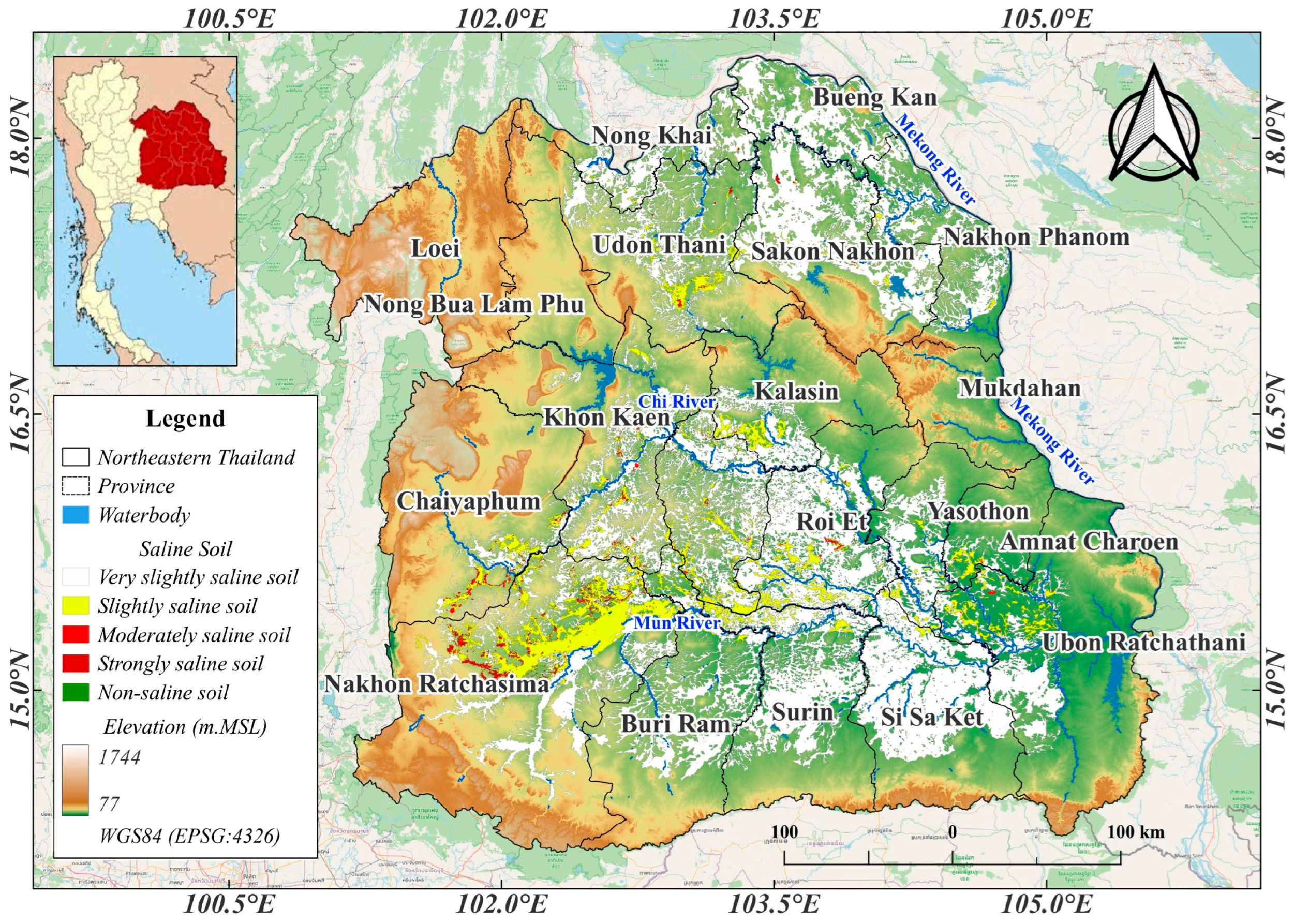
Figure 1. Map of the study area in Northeastern Thailand.
Geomatics 05 00080 g001
Figure 2. NDVI and EVI dynamics across rice growth phases.
Geomatics 05 00080 g002
Figure 3. Rice yield sample collection process: (a) Locating rice yield collection points using RTK GNSS; and (b) sorting of rice yield samples in preparation for weighing.
Geomatics 05 00080 g003
Figure 4. Distribution of rice yield sampling points and paddy fields in the study area.
Geomatics 05 00080 g004
Figure 5. Process of saline soil sample collection: (a) Field collection of saline soil samples; and (b) coordinate data collection at saline soil sampling sites using RTK GNSS network. These data were used to verify the field data.
Geomatics 05 00080 g005
Figure 6. The distribution of EC sampling points in the study area.
Geomatics 05 00080 g006
Figure 7. Flow chart of the methodology used in this study for rice yield mapping.
Geomatics 05 00080 g007
Figure 8. Flow chart of the methodology used in this study for soil salinity mapping.
Geomatics 05 00080 g008
Figure 9. Seasonal trends of NDVI and EVI in relation to rice growth stages (from land preparation to harvest). X-axis shows rice growth period (Jul–Dec); Y-axis shows NDVI and EVI. Shaded areas show data variability.
Geomatics 05 00080 g009
Figure 10. Model performance (R2 and RMSE) across varying numbers of features for rice yield prediction using Random Forest (RF), Support Vector Regression (SVR), and Classification and Regression Trees (CART) on the Fusion, Landsat-8, and Sentinel-2 datasets: (ac) RF with Fusion, Landsat-8, and Sentinel-2; (df) SVR with Fusion, Landsat-8, and Sentinel-2; (gi) CART with Fusion, Landsat-8, and Sentinel-2. The X-axis represents the number of selected features, while the left Y-axis shows the coefficient of determination (R2) and the right Y-axis shows the RMSE. The solid black and dashed red lines indicate R2 and RMSE, respectively.
Geomatics 05 00080 g010
Figure 11. Pearson correlation of median NDVI and EVI (August–November): (a) Sentinel-2 dataset, (b) Landsat-8 dataset. Color scale: green positive, white weak, red negative correlation with rice yield.
Geomatics 05 00080 g011
Figure 12. Top five features selected for rice yield prediction using machine learning models on the Fusion, Landsat-8, and Sentinel-2 datasets: (a) RF, (b) CART, and (c) SVR. L8_ denotes indices from Landsat-8, S2_ from Sentinel-2, and numbers (08–11) indicate acquisition months (August–November).
Geomatics 05 00080 g012
Figure 13. Variable importance ranking of the top five predictors derived from the Random Forest (RF) model using the Fusion dataset.
Geomatics 05 00080 g013
Figure 14. Spatial distribution of rice yield predictions in Northeastern Thailand generated using machine learning models with Landsat-8, Sentinel-2, and Fusion datasets. (ac) Landsat-8 results using RF, SVR, and CART; (df) Sentinel-2 results using RF, SVR, and CART; (gi) Fusion results using RF, SVR, and CART. The color scale represents rice yield (t ha−1), ranging from red (low yield) to dark green (high yield).
Geomatics 05 00080 g014
Figure 15. Model performance (R2 and RMSE) across varying numbers of features for soil salinity estimation: (ac) RF with Fusion, Landsat-8, and Sentinel-2; (df) SVR with Fusion, Landsat-8, and Sentinel-2; (gi) CART with Fusion, Landsat-8, and Sentinel-2. The X-axis represents the number of selected features, while the left Y-axis shows the coefficient of determination (R2) and the right Y-axis shows the RMSE. The solid black and dashed red lines indicate R2 and RMSE, respectively.
Geomatics 05 00080 g015
Figure 16. Correlation heatmap of Landsat-8 spectral bands, vegetation indices, and EC.
Geomatics 05 00080 g016
Figure 17. Correlation heatmap of Sentinel-2 spectral bands, vegetation indices, and EC.
Geomatics 05 00080 g017
Figure 18. Top five features selected for soil salinity models using machine learning models on the Fusion, Landsat-8, and Sentinel-2 datasets: (a) RF, (b) CART, and (c) SVR. L8_ refers to indices from Landsat-8, and S2_ refers to indices from Sentinel-2, both representing spectral or salinity-related features.
Geomatics 05 00080 g018
Figure 19. Variable importance ranking of the top five predictors derived from the Random Forest (RF) model using the Fusion dataset for soil salinity prediction.
Geomatics 05 00080 g019
Figure 20. Spatial distribution maps of soil electrical conductivity (EC, dS/m) in Northeastern Thailand generated using machine learning models with Landsat-8, Sentinel-2, and Fusion datasets. (ac) Landsat-8-based results using RF, SVR, and CART; (df) Sentinel-2-based results using RF, SVR, and CART; (gi) Fusion based results using RF, SVR, and CART. The color scale represents soil electrical conductivity (EC, dS/m), ranging from green (low salinity) to red (high salinity).
Geomatics 05 00080 g020
Figure 21. Data distribution reflecting the relationship between rice yield and soil electrical conductivity (EC) during the seedling stage (dS/m). The red curve represents the polynomial regression model, while the blue dots indicate sample data linking soil EC (dS/m) during the seedling stage with rice yield (t ha−1). The histograms illustrate the data distribution, revealing a trend of decreasing rice yield with increasing EC values.
Geomatics 05 00080 g021
Table 1. Spectral indices derived from Landsat-8 and Sentinel-2 imagery for rice yield estimation and soil salinity assessment.
DataVegetationFormulaReference
Landsat-8Normalized Difference Vegetation Index (NDVI) N I R R e d N I R + R e d [44]
Enhanced Vegetation Index (EVI) 2.5 × N I R R e d N I R + 6 × R e d 7.5 × B l u e + 1 [45]
Soil Adjusted Vegetation Index (SAVI) N I R R e d × 1.5 N I R + R e d + 0.5 [47]
Normalized Difference Water Index (NDWI) G r e e n N I R G r e e n + N I R [48]
Green Normalized
Difference Vegetation
Index (GNDVI)
N I R G r e e n N I R + G r e e n [49]
Sentinel-2Normalized Difference Vegetation Index 1 (NDVI) B 8 B 4 B 8 + B 4 [44]
Normalized Difference Water Index (NDWI) B 3 B 8 B 3 + B 8 [48]
Enhanced Vegetation Index (EVI) 2.5 × B 8 B 4 B 8 + 6 × B 4 7.5 × B 2 + 1 [45]
Soil Adjusted Vegetation Index (SAVI) B 8 B 4 × 1.5 B 8 + B 4 + 0.5 [47]
Salinity Index 1 (SI1) B 2 × B 4 [50]
Salinity Index 2 (SI2) B 3 × B 4 [50]
Salinity Index 3 (SI3) B 3 2 + B 4 2 [51]
Salinity Index 4 (SI4) B 2 × B 4 B 3 [52]
Salinity Index 5 (SI5) B 3 + B 4 2 [51]
Table 2. Spectral–temporal datasets used for training and testing of rice yield prediction models.
DatasetSourceSpectral–Temporal Data
1Landsat-8Seasonal: NDVI and EVI
2Sentinel-2Seasonal: NDVI and EVI
3Landsat-8 + Sentinel-2Seasonal: (S-2) NDVI and EVI, (L-8) NDVI and EVI
Table 3. Spectral–temporal datasets used for soil salinity mapping.
DatasetSourceSpectral–Temporal Data
1Landsat-8B2-B7, NDVI, SAVI, EVI, GNDVI, NDWI, SI1-SI5
2Sentinel-2B2-8A, B11-12, NDVI, SAVI, EVI, GNDVI, NDWI, SI1- SI5
3Landsat-8 + Sentinel-2L8: B2-B7, S2: B2-8A, B11-12, NDVI, SAVI, EVI, GNDVI, NDWI, SI1-SI5 S2: B2-B8A, SI1-SI5
Table 4. Performance of machine learning models for rice yield prediction.
DatasetRandom Forest (RF)Classification and Regression Trees (CART)Support Vector Regression (SVR)
TrainingValidationTrainingValidationTrainingValidation
R2RMSER2RMSER2RMSER2RMSER2RMSER2RMSE
10.960.100.820.210.800.220.680.280.800.330.650.37
20.830.130.640.300.630.300.500.350.720.390.600.42
30.970.090.860.190.820.210.700.260.810.290.720.33
Table 5. Performance of machine learning models for soil salinity estimation.
DatasetRandom Forest (RF)Classification and Regression Trees (CART)Support Vector Regression (SVR)
TrainingValidationTrainingValidationTrainingValidation
R2RMSER2RMSER2RMSER2RMSER2RMSER2RMSE
10.970.620.831.360.891.170.781.640.891.260.771.68
20.960.650.811.460.801.560.761.640.801.720.761.82
30.980.380.930.870.930.930.851.330.911.080.811.35
Table 6. Summary statistics of rice yield and EC during the seedling stage.
Count Mean Std Min Max
Yield (ton/ha)50002.820.601.013.71
EC during the seedling stage (dS/m)50005.983.763.1522.32
Disclaimer/Publisher’s Note: The statements, opinions and data contained in all publications are solely those of the individual author(s) and contributor(s) and not of MDPI and/or the editor(s). MDPI and/or the editor(s) disclaim responsibility for any injury to people or property resulting from any ideas, methods, instructions or products referred to in the content.