Abstract
This article addresses the issue of designing compound curves, i.e., a geometric system consisting of two (or more) circular arcs of different radii, pointing in the same direction and directly connected to each other. Nowadays, compound curves are mainly used on tram lines; they also occur on railways (e.g., on mountain lines), but new ones are generally no longer being built there. Therefore, in relation to railway lines, the aim is to be able to recreate (i.e., model) the existing geometric layout with compound curves, so that it is then possible to correct this layout. An analytical method for designing track geometric systems was used, adapted to the mobile satellite measurement technique, in which calculations are carried out in the appropriate local Cartesian coordinate system. The basis of this system is the symmetrically arranged adjacent main directions of the route, and the beginning is located at the point of intersection of these directions. A number of detailed issues have been clarified and basic characteristic quantities have been determined, and the computational algorithm described in the paper leads to the solution of the problem in a sequential manner. The obtained possibilities of modeling the compound curves are illustrated by the provided calculation example.
1. Introduction
The field of railway engineering has a very long history; this also applies to the methods used to design track geometrical systems. Due to limited computational capabilities, numerous simplifying assumptions have been introduced over the decades, a classic example of which is the transition curve in the form of a third-degree parabola (i.e., simplified clothoid) used to this day. The progress of electronic computing technology, which occurred in the second half of the 20th century, radically changed this situation and led to the development of computational algorithms that strictly correspond to a specific geometric situation. As a result, for many years, the development of design documentation in the field of railways has been carried out using commercial computer software [1,2]. The belief has therefore become stronger so that conducting research work on the methodology of designing track geometrical systems is now less important. Of course, such work is carried out [3,4,5], but its scope is often limited to detailed issues, such as transition curves [6,7,8,9,10] or railway turnouts [11,12,13,14,15,16].
Due to the competitive conditions with other transport systems, new railway lines are usually adapted to the increased speed of trains; in fact, a significant part of them are high-speed railways. On the other hand, traditional lines (existing, most often built in the 19th century) are disappearing from the field of research interest, as they would have to be modified to adapt to contemporary requirements. This especially applies to railway lines running in difficult terrain conditions (e.g., in mountainous terrain), where there are small radii of horizontal curves, and additionally controversial geometric arrangements, such as compound curves and reverse curves. Improving the quality of these lines, leading to an increase in travel speed, requires appropriate modernization activities. In the case of compound curves and reverse curves, this would consist in introducing transition curves between the occurring horizontal curves.
This article addresses the issue of designing compound curves, i.e., a geometric system consisting of two consecutive circular arcs of different radii, pointing in the same direction and directly connected to each other. Compound curves are currently used on tram lines. They were used on railways until the middle of the last century; after that, they were basically no longer made there. However, those built earlier still exist on many railway lines, creating specific operational problems caused by the sudden changes in curvature that occur on them. To a lesser extent, they were also affected by the progress in computational technology that occurred later. The design of compound curves differs in its level from the situation related to other geometric systems. From the scientific point of view, the interest in the discussed problem is relatively small, and the practical aspects of the issue are rather exposed [17].
The lack of transition curves at the connection of both circular arcs introduces disturbances in the mechanical system of the rail vehicle—track, which results in driving discomfort for passengers and the increased lateral wear of the rails. Therefore, in relation to railway lines, the aim is to obtain the possibility of reproducing (i.e., modeling) the existing geometric layout with compound curves, so that it is then possible to correct the horizontal ordinates in the area where the circular arches connect. For this purpose, it was necessary to develop an effective method for designing such a system, which, however, by assumption, will not be used to determine the coordinates of a new compound curve, but to model the existing system (with a view to its later modification).
At this point, it should be noted that the analytical method of designing compound curves had already been developed and presented in [18]. It concerned a model solution, i.e., creating a geometric system from scratch, in which circular arcs of different radii are connected with each other by means of an appropriate transition curve. A classic compound curve, in which the transition curve does not occur, was a special case in this method. The issue of modifying the existing geometric system was not considered. Meanwhile, as it seems, the real problem lies somewhere else. After all, it is not about creating new model systems of compound curves (with appropriate transition curves), but modernizing the existing systems. In this situation, the classic compound curve becomes the subject of interest.
The inspiration for developing an analytical method for designing track geometric systems came from new possibilities in the field of measurement technology, related to the use of mobile satellite measurements [19]. They consist in driving a given railway route with satellite antennas installed on the pivots of the rail vehicle bogies. As a result, one obtains—in a very short time—the Cartesian coordinates of the track axis points in the appropriate global system. In Poland—in relation to flat coordinates—it is the national spatial reference system PL-2000 [20]. The designated track axis coordinates allow for the easy determination of the main directions of the route (as simple least squares), while the areas of changes in the main directions should be designed in the appropriate local coordinate systems, using mathematical notation. In this way, the entire railway route consists of straight sections (established or determined on a measurement path) and areas of their mutual connection, the coordinates of which result from the transformation of the appropriate geometric system from the local coordinate system to the global system.
The developed analytical method allowed for considering many different detailed issues, often constituting the only effective way to conduct the relevant analysis. In addition to the design of the areas of changes in the main directions of the route [21,22,23], it was used in the analysis of transition curves and methods of their extension [9,24,25], the arching of railway turnouts and shaping their diverging track [26,27,28], widening the intertrack space [29] and determining the horizontal curvature of the track axis using the moving chord method [30,31,32].
The standard procedure of the analytical design method in its previous versions [21,22,23] is basically carried out in the local coordinate system and is characterized—in its initial phase—by the lack of knowledge of the location of the origin of this system in relation to the global coordinate system. Full integration of both of these systems requires carrying out the design procedure in the local system until the very end. The location of the origin of this system in relation to the appropriate main point of the route and its resulting coordinates in the global system are determined only in the final phase of the procedure. This may constitute the basic methodological reservation to the discussed design method. For this reason, certain interpretation problems may also arise.
As it turns out, these difficulties can be avoided by locating the origin of the local coordinate system at the point of intersection of both the main directions of the route, whose Cartesian coordinates in the global system are known. Such a version of the analytical design method was presented in [33]; it is universal in nature and covers the areas of connection of adjacent main directions of the railway route (both symmetrical and asymmetrical). In this paper, an analogous approach was used in the design of classic compound curves. Therefore, a similar sequential procedure was adopted as in [33]. It includes the following items:
- (a)
- Rules for creating a local coordinate system;
- (b)
- Determination of basic computational quantities;
- (c)
- Connection of both horizontal arches;
- (d)
- Transferring the solution to the local coordinate system;
- (e)
- Considerations regarding computational algorithms;
- (f)
- Determination of coordinates in the global system (presented in the appropriate calculation example).
Compared to the work in [33], a shortened version of the principles of creating a local coordinate system has been retained for illustrative purposes; however, due to the specificity of the problem under consideration, item (b) has been significantly extended, item (c) concerns connecting two arcs with different radii, item (d) is similar, and items (e) and (f) refer to a completely different issue.
2. Local Coordinate System
Similarly to other variants of the analytical design method, when designing classic compound curves (in which horizontal arcs of different radii are directly connected to each other), it was assumed that the design of a given area of route direction change will be carried out in the appropriate local Cartesian coordinate system x, y (marked as LCS). The basis of this system is the symmetrically set adjacent main directions. In order to obtain such a setting of the main directions, an appropriate transformation (i.e., shift and rotation) of the global system must be performed.
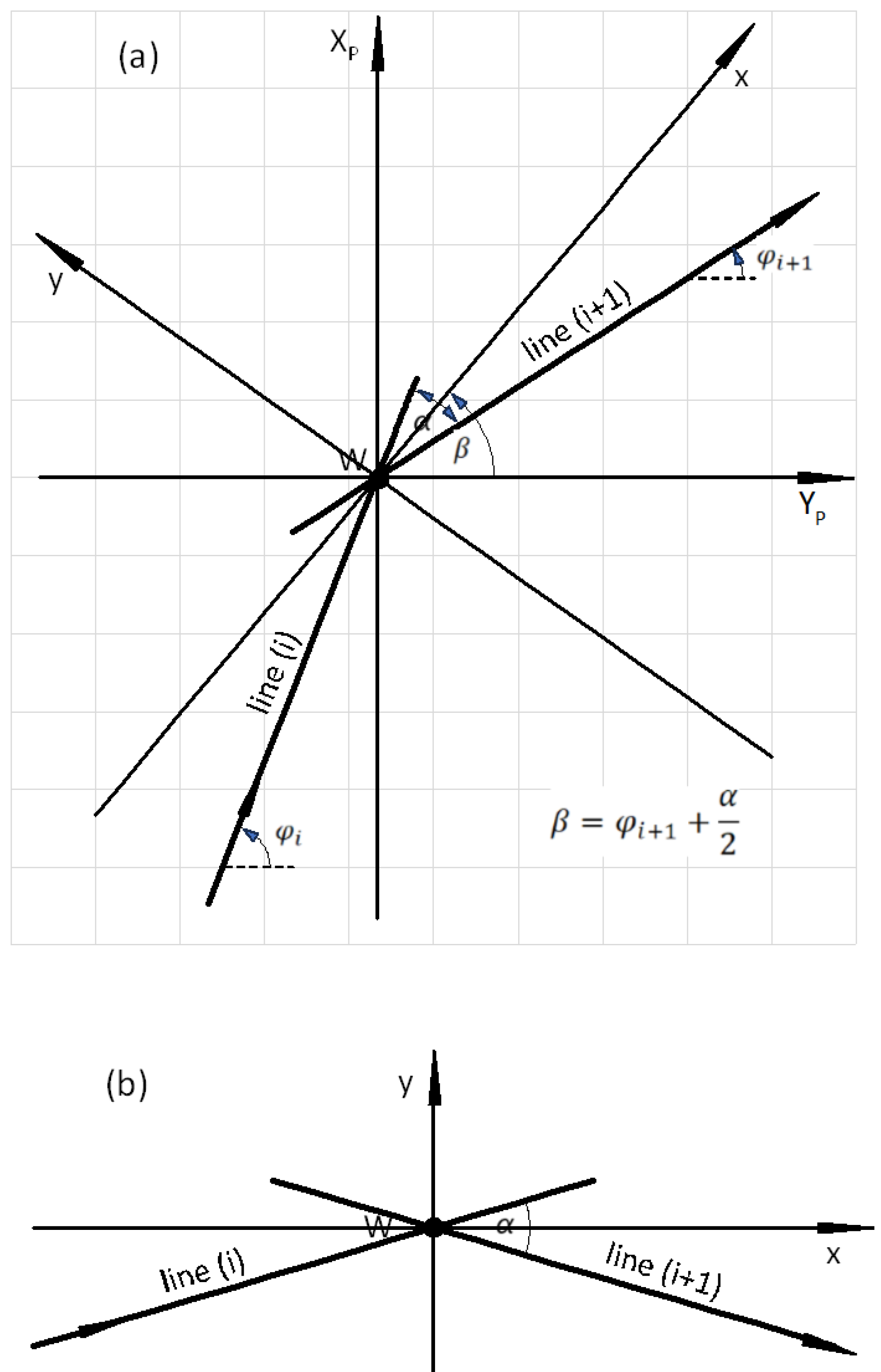
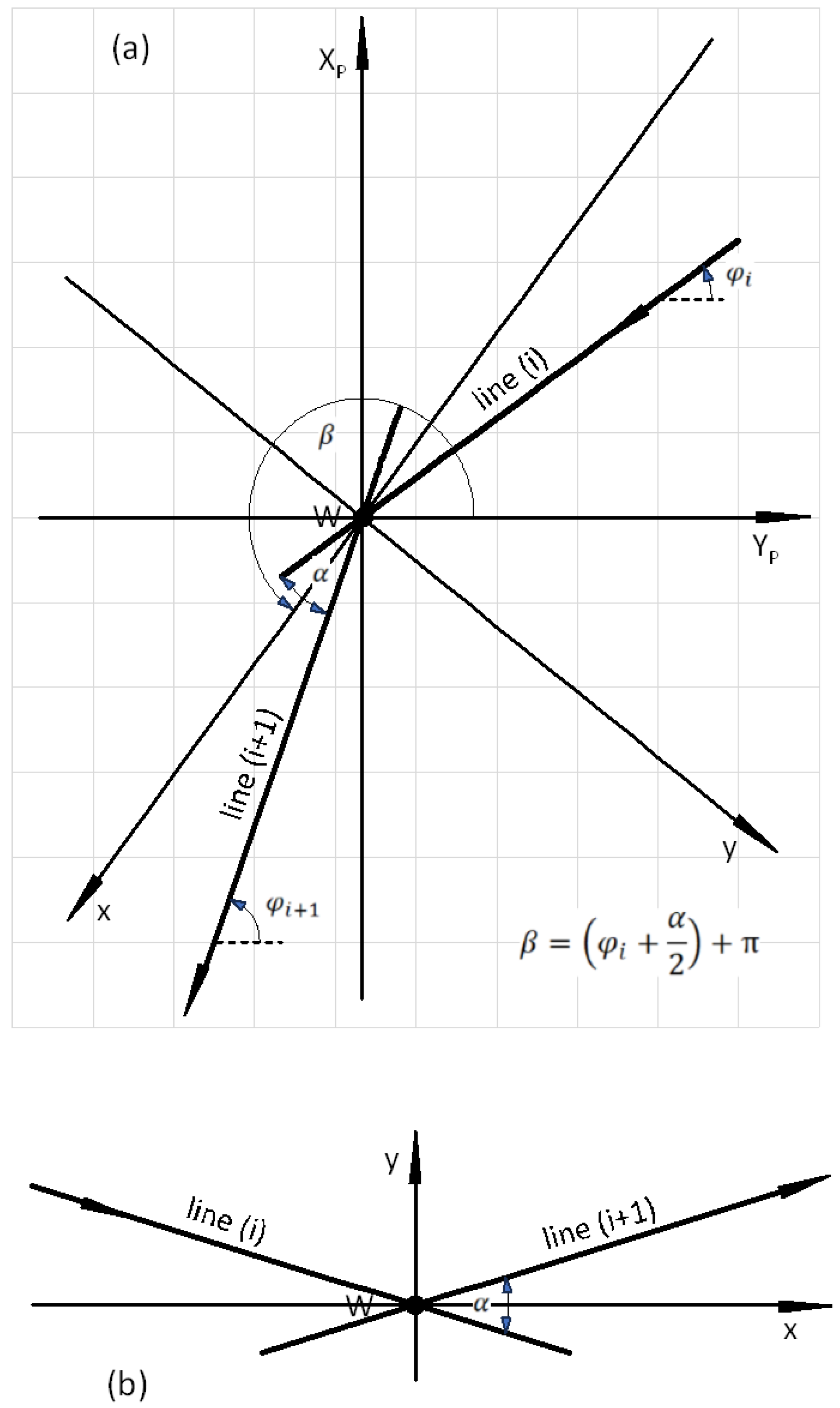
Design activities carried out in the global rectangular coordinate system, i.e., creating a polygon of the main directions of the route and determining the mathematical equations of these directions, the coordinates of their intersection points (i.e., main points) and the angles of return, were presented in [33]. This work also explains the method of creating a local coordinate system for a given area of changing the route direction, consisting in shifting the origin of the global system to the point of intersection of two adjacent main directions (i.e., to point W), and then rotating the shifted system YP, XP by such an angle β as to obtain a symmetrical setting of the main directions in the local coordinate system x, y. Examples of this operation are shown in Figure 1 and Figure 2.
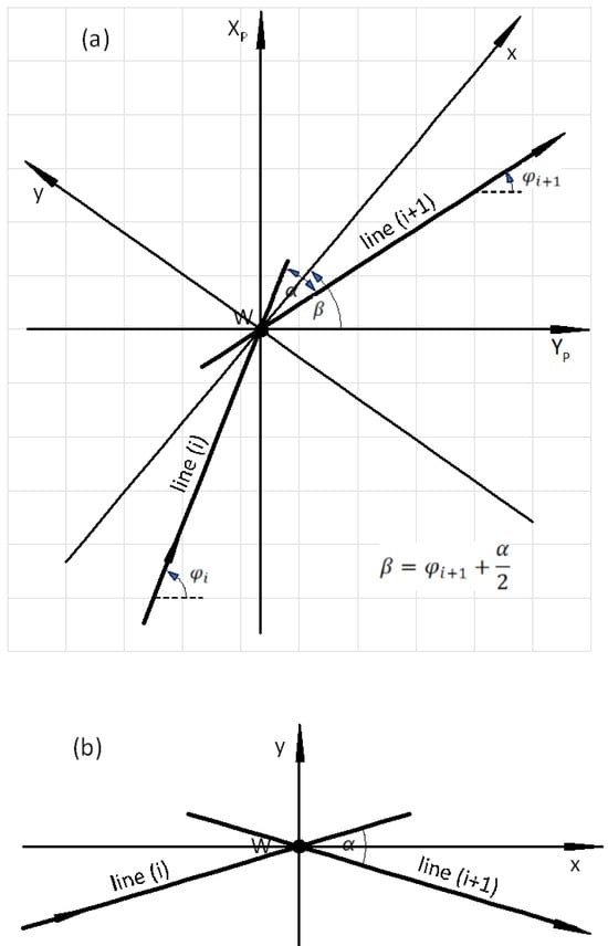
Figure 1.
(a) Local coordinate system x, y against the background of the intersecting main directions of the route in the shifted PL-2000 system (with the kilometer running from left to right); (b) System x, y after the transformation.
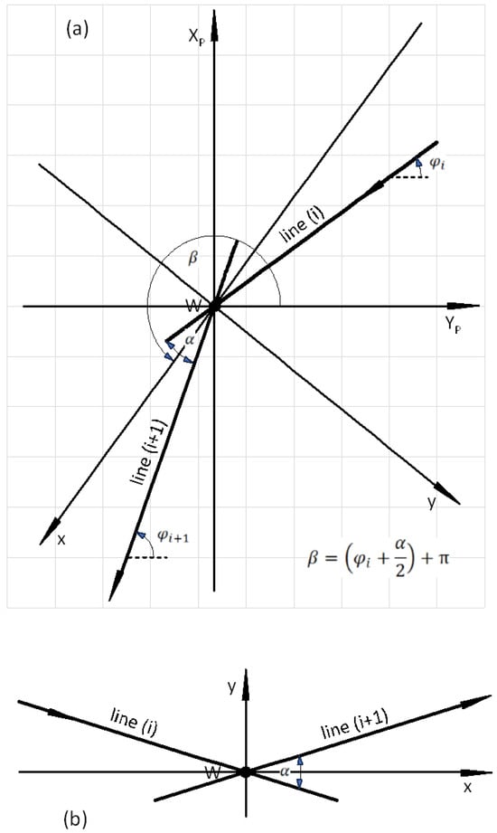
Figure 2.
(a) Local coordinate system x, y against the background of the intersecting main directions of the route in the shifted PL-2000 system (with the kilometer running from right to left); (b) System x, y after the transformation.
It should be noted that the setting of the main directions of the route in the PL-2000 system can be very diverse; Figure 1a and Figure 2a show only two selected cases. However, after the transformation to the local coordinate system (as shown in Figure 1b and Figure 2b), there are only two possibilities for locating the designed geometric system: under the x axis, with negative ordinates and the convexity of the curvilinear elements directed upwards, and above the x axis, with positive ordinates and the convexity of the curvilinear elements directed downwards. Therefore, when considering the procedure in detail, it is necessary to present the computational algorithms related to these two situations. This means that, when determining the formulas for the coordinates of characteristic points in the local coordinate system, two possible cases should be taken into account:
This paper presents the procedure for creating a geometric system covering Case I. The design of the geometric system is carried out in several stages, which are presented later in the article.
3. Determination of Basic Calculation Quantities
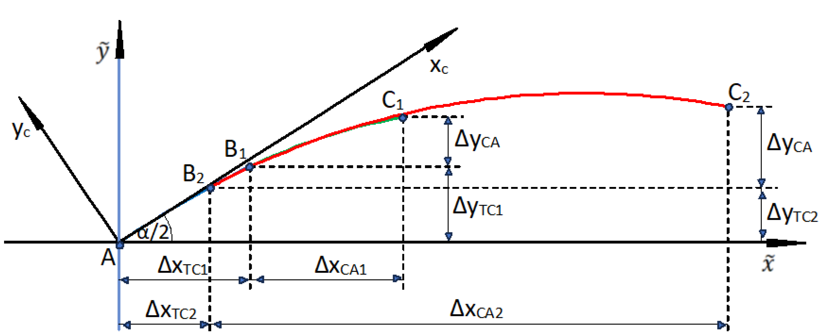
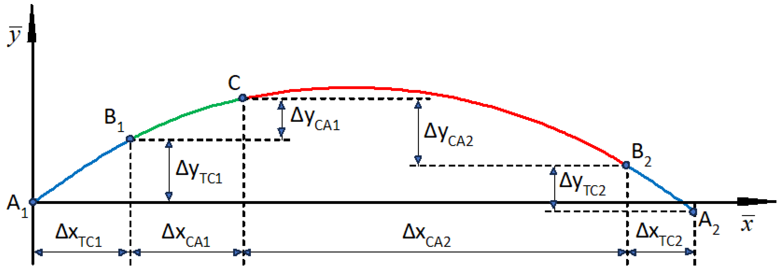
In order to be able to operate in the local coordinate system, it is necessary to first perform an auxiliary procedure, which aims to determine the basic calculation quantities. These quantities refer to the regions of the geometric system connecting the ends of the extreme straight segments (i.e., the beginnings of the transition curves) with the connection point of both circular arcs. This refers to the lengths of the projections of the transition curve () and the circular arc () on the horizontal axis, as well as the lengths of the projections of the transition curve () and the circular arc () on the vertical axis. The calculations of the searched parameters, separately for both occurring horizontal arcs, are carried out in the system shown in Figure 3.
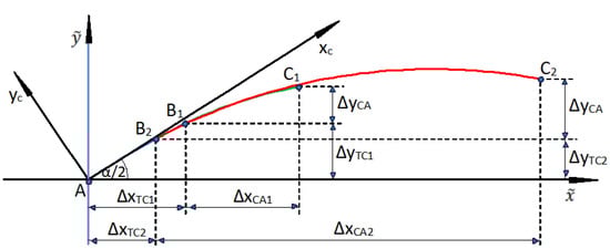
Figure 3.
Scheme for determining the basic characteristic quantities of a geometric system (the CA1 circular arc is marked in black, and the CA2 arc is marked in red).
We start by drawing a straight line simulating the main direction i through point A(0, 0) in coordinate system ; it is described by the equation
This straight line is the abscissa axis of the coordinate system xc, yc, associated with the transition curve of length lc, which is connected to a circular arc of radius R. We are interested in the coordinates of the end point of the curve in this system, which result from the corresponding parametric equations xc(l) and yc(l) for l = lc. In the case of using the transition curve in the form of a clothoid, these coordinates are as follows:
while the angle Θc(lc) of inclination at the end of the curve is determined from the dependence
The transformation of the transition curve to the coordinate system is performed by rotating the reference system by an angle of α/2. The appropriate formulas depend on the direction of rotation. As a result of this operation, the required value of the projection of the transition curve onto the horizontal and vertical axes is obtained. In the case of a right rotation of the xc, yc system (as in Figure 3), the following values are obtained:
The value of the tangent at the end is described by the formula
Knowing the position of the transition curve, we can inscribe a circular arc of radius R in the geometric system. The center of this arc (point S) lies on the line perpendicular to the tangent at the end of the transition curve (i.e., at point B), at a distance R from this point. The coordinates of point S are as follows:
A circular arc is described by the equation
and the value of the tangent to the geometric system is
The important characteristic point is point H, where the slope of the tangent to the geometric system is zero (i.e., = 0). Its coordinates are as follows: , . The connection of both circular arcs (i.e., point C) should be located to the left or right of point H. The condition must be met.
The value of the abscissa of point C results from the arbitrarily assumed difference relating to a circular arc of radius R1; it is
The ordinate of this point is determined based on Equation (10).
The difference for the circular arc CA1, associated with the first transition curve (TC1), is determined from the formula
The key quantity for further actions is the slope of the tangent at point C, which is the same for both connected arcs. It is
When constructing the entire circular arc, the differences and for the transition curve TC1 (determined using Formulas (5) and (6)) should be used, as well as the arbitrarily assumed difference and difference (determined by Formula (14)) for the circular arc CA1. After entering the radius R2, the differences and for the transition curve TC2 are obtained. Determining the values and for the circular arc CA2 requires an additional calculation procedure.
Knowing the position of the transition curve TC2 in the system shown in Figure 3, we can inscribe a circular arc of radius R2 in the geometric system. The coordinates of the center of this arc (i.e., point S2) result from Equations (8) and (9). In the coordinate system, the second circular arc is also described by Equation (10), and the value of the tangent at its end by Equation (11).
In the target geometric system (i.e., in a compound curve), this arc will be mirrored relative to the abscissa , so the tangent at its end point must satisfy the condition
The indices S1 and S2 appearing in the designations and indicate that the given quantity applies to point S1 and S2, respectively. The adopted convention also applies to the other characteristic points used.
After taking into account Formula (12), we obtain
The right-hand side of the above expression is already known at this stage, as it results from Equation (15). Therefore, we need to solve the following equation with the unknown :
As a result of this operation, we obtain:
The coordinates of the end of the second circular arc are as follows:
The difference is determined by the formula
The position of a circular arc of radius R2 in the system, with marked the differences and , is shown in Figure 3.
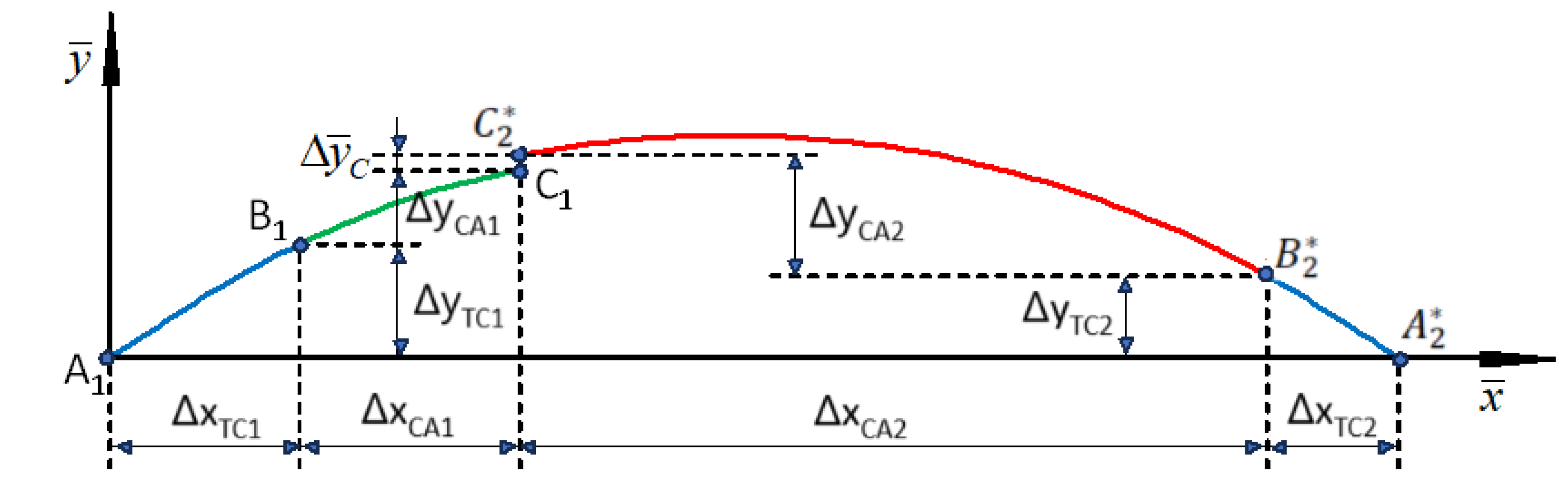
4. Connection of Both Horizontal Arcs
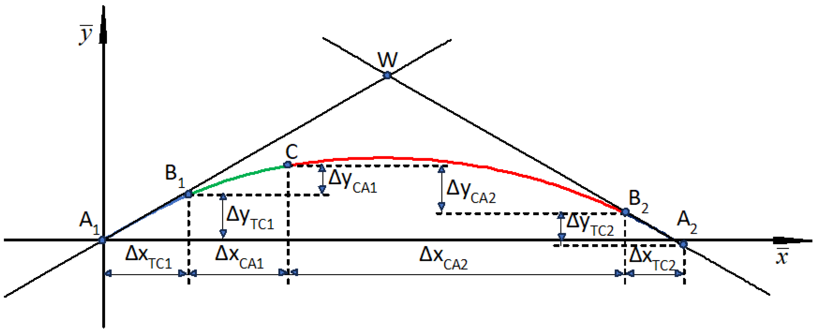
The construction of a compound curve, i.e., connecting the existing horizontal arcs with radii R1 and R2, will be performed in the auxiliary coordinate system shown in Figure 4. The case of a geometric system located below the vertex W (i.e., shown in Figure 1) was considered.
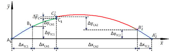
Figure 4.
Geometric system created as a result of mirror reflection of TC2 and CA2 with respect to the abscissa (the transition curves TC1 and TC2 are marked in blue, the CA1 circular arc in green, and the CA2 arc in red).
For the transition curve TC1 and the circular arc CA1, this system is identical to the system ; this means that and . Therefore, the coordinates of the characteristic points are:
For the TC2 curve and the CA2 arc, it will be necessary to perform an appropriate transformation, consisting in performing a mirror reflection with respect to the abscissa . The characteristic points , , and , obtained as a result of this operation, do not yet occupy their final position and will require correction. Their coordinates are as follows:
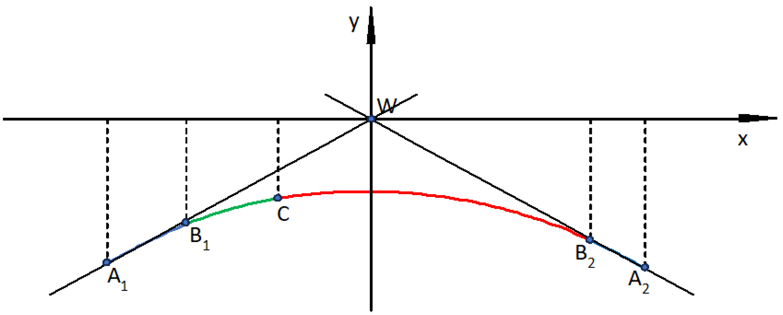
As can be seen in Figure 4, at the assumed connection point of both arcs, there is a difference in ordinates , which is
In order to obtain a smooth connection of both parts of the geometric system, the ordinates of this system related to the arc of radius R2 should be corrected (while maintaining the abscissa values). For Case I, we obtain
Figure 5 shows the geometric system of the corresponding compound curve in the coordinate system.
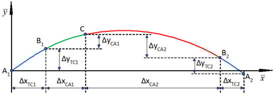
Figure 5.
Geometric system for Case I created after correcting the TC2 and CA2 ordinates from Figure 4 (the transition curves TC1 and TC2 are marked in blue, the CA1 circular arc in green, and the CA2 arc in red).
For the geometric system located above the vertex W (Case II in Figure 2b), the same formulas for the abscissa values apply, but the ordinates take negative values. This means that
5. Transferring the Solution to the Local Coordinate System
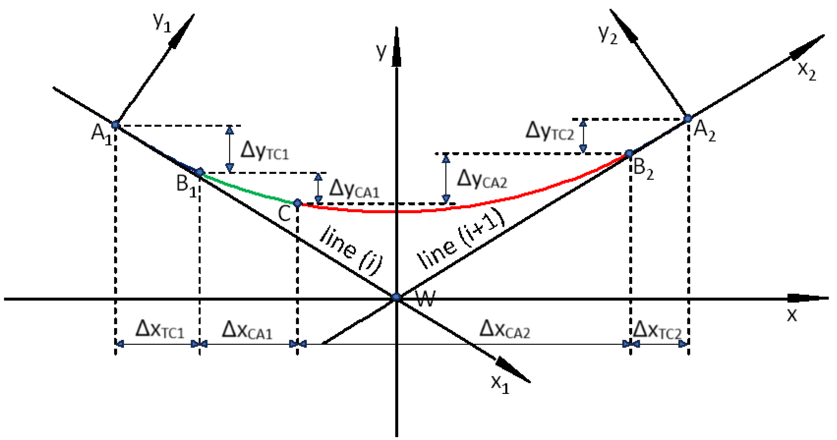
Knowing the coordinates of the extreme points of the geometric system A1(0,0) and , we can transfer the obtained solution to the local coordinate system x, y (shown in the given case in Figure 1b). To do this, we need to derive from these points two tangent lines inclined at an angle α/2—positive from point A1 and negative from point A2 (Figure 6). The equations of these lines are as follows:
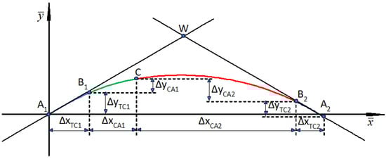
Figure 6.
Geometric system of the compound curve against the background of the introduced main directions of the route (the transition curves TC1 and TC2 are marked in blue, the CA1 circular arc in green, and the CA2 arc in red).
The intersecting point of lines (21) and (22) is the origin of the local coordinate system. Its coordinates in the system are as follows:
In Case II, the coordinates of point W are described by the formulas:
Thanks to their knowledge, it is possible to transform the points of the geometric system into the local coordinate system using the formulas:
Figure 7 shows the geometric system of the compound curve from Figure 6 transferred to the local coordinate system.

Figure 7.
Geometric system of the compound curve in the local coordinate system (the transition curves TC1 and TC2 are marked in blue, the CA1 circular arc in green, and the CA2 arc in red).
Knowing the assumed values of the radii R1 and R2 of the compound curve and the lengths l1 and l2 of the transition curves, one must first determine—using the appropriate formulas—the values and , and , and , and , and and . In the local coordinate system x, y, the beginning of the transition curve TC1 (point A1) is located in the main direction (i), and the beginning of the curve TC2 (point A2) is located in the main direction (i + 1). The list of formulas for the coordinates of all characteristic points is provided in Table 1.

Table 1.
List of formulas for the coordinates of characteristic points.
The values and appearing in Table 1 result from Formulas (23)–(26), and from Formula (20).
6. Considerations for Computational Algorithms
After determining the coordinates of the characteristic points, the design process should be finalized by determining the course of the route sections located between these points. The calculations used for this purpose are sequential and do not require any iterations. Therefore, due to the simplicity of the calculation algorithms, the article does not provide a full flowchart of the calculation procedure, limiting itself to providing a list of the required formulas. It was necessary to take into account the diversity of calculation algorithms related to the directions of rotation of the coordinate systems related to the transition curves. In practice, this involves the separate determination of coordinates in the x, y system for the geometric system located below the W vertex (i.e., for Case I) and above the W vertex (i.e., for Case II). In Case I, the situation is shown in Figure 8, while in Case II—the situation is shown in Figure 9.
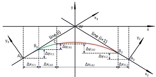
Figure 8.
Designed compound curve in the local coordinate system for the case of the geometric system located below the W vertex (the transition curves TC1 and TC2 are marked in blue, the CA1 circular arc in green, and the CA2 arc in red).

Figure 9.
Designed compound curve in the local coordinate system for the case of the geometric system located above the W vertex (designations of transition curves and circular arcs as in Figure 8).
To determine the computational algorithms, we must first determine the coordinates of the centers of both connected arcs in the local coordinate system. This is performed using the knowledge of the computational parameters of point C—the abscissa xC, the ordinate yC, and the slope of the tangent sC. The centers of both arcs (points S1 and S2) lie on the line perpendicular to the tangent at point C, at distances R1 and R2 from this point. The corresponding formulas are presented in Table 2. In the formulas for the abscissa values, the sign of the slope of the tangent sC plays an important role.
Table 2.
List of formulas for the coordinates of the centers of connected circular arcs.
Table 3 presents a list of formulas necessary to determine the coordinates of individual elements of the designed geometric system. It includes the following:
Table 3.
List of formulas for determining the coordinates of a geometric system.
- Parametric equations of the transition curve TC1 in the auxiliary x1, y1 coordinate system (for );
- Equation of the angle of inclination of the tangent in the x1, y1 auxiliary coordinate system (for );
- Parametric equations of the transition curve TC1 in the local coordinate system x, y (for );
- Formula for the tangent value at the end of the transition curve TC1;
- Equation of a circular arc CA1 with radius R1;
- Equation of a circular arc CA2 with radius R2;
- Parametric equations of the transition curve TC2 in the auxiliary x2, y2 coordinate system (for );
- Equation of the angle of inclination of the tangent in the auxiliary x2, y2 coordinate system (for );
- Parametric equations of the transition curve TC2 in the local coordinate system x, y (for );
- Formula of the tangent value at the end of the transition curve TC2.
7. Calculation Example
In the presented calculation example, a system of main directions of the route was assumed, intersecting at point W, whose coordinates in the PL-2000 system are YW = 6,751,176.928 m, XW = 6,249,641.342 m. We are dealing with a turn of the route to the left, with increasing mileage from right to left (which corresponds to the situation in Figure 2).
The assumed train speed on the designed compound curve is V = 90 km/h. This results from the smaller radius of the circular arc R2 = 450 m and the cant h2 = 125 mm, where the unbalanced acceleration is am = 0.571 m/s2 (the permissible value aper = 0.6 m/s2 was adopted). The length of the corresponding transition curve in the form of a clothoid is l2 = 115 m (the wheel lifting speed on the gradient due to cant is f = 27.174 mm/s; the permissible value fper = 28 mm/s was adopted). The circular arc radius R1 = 600 m and cant h1 = 75 mm were assumed, which determines the unbalanced acceleration am = 0.551 m/s2. The length of the transition curve in the form of a clothoid is l1 = 75 m (the wheel lifting speed on the gradient due to cant is f = 25.000 mm/s). In the PL-2000 system, the straight line representing the main direction (i) is described by the formula
and the line describing the direction (i + 1) by equation
From the given equations of the main directions, it follows that the angles of inclination of the lines are φi = 0.324 rad and φi+1 = 1.258 rad. On this basis, the angle of return of the route α = φi+1 − φi = 0.934 rad.
Obtaining the local coordinate system x, y, with symmetrically set adjacent main directions, requires shifting the origin of the PL-2000 system to point W and rotating it with respect to this point to the left by an angle β = (φi + α/2) + π = 3.284 rad. In the coordinate system x, y, the angles of inclination of the straight lines will be = −α/2 = −0.467 rad, = α/2 = 0.467 rad.
The actual design begins with an auxiliary operation to determine the coordinates of characteristic points using the formulas given in Chapter 3. The following values were obtained: = 67.646 m, = 32.358 m, = 0.428108, = 300 m (assumed value), = 45.012 m, = 104.721 m, = 47.321 m, = 0.352862, = 101.841 m and = 23.087 m. The formulas given in Table 1 allowed us to determine the coordinates of points A1, B1, C, B2 and A2 (Figure 8). The values of these coordinates (and the tangents) are given in Table 4.
Table 4.
The values of the parameters of the characteristic points for the geometric system in the presented calculation example.
Further design operations are performed in the local coordinate system x, y, using the formulas given in Table 3. First, an auxiliary coordinate system x1, y1 is assumed, related to the transition curve TC1. The beginning of this curve (i.e., point A1) is also the beginning of the designed geometric system. The clothoid coordinates x1(l) and y1(l) were determined for m. The value of the angle of inclination of the tangent at the end of the curve was Θ1(l1) = −0.0625 rad. The next stage of the operations is to rotate the system x1, y1 to the right by an angle α/2. For the parametric equations x(l) and y(l) of the curve TC1, the condition m applies. The coordinates of the circular arc related to the curve TC1 were determined for m.
Then, the auxiliary coordinate system x2, y2, related to the transition curve TC2, was used. The beginning of this curve (i.e., point A2) is the end of the designed geometric system. The clothoid coordinates x2(l) and y2(l) were determined for m. The value of the angle of inclination of the tangent at the end of the curve was Θ2(l2) = −0.12778 rad. As a result of rotating the system x2, y2 to the left by an angle α/2, the parametric equations x(l) and y(l) of the curve TC2 were obtained, and the condition m is valid. The coordinates of the circular arc related to the curve TC2 were determined for m.
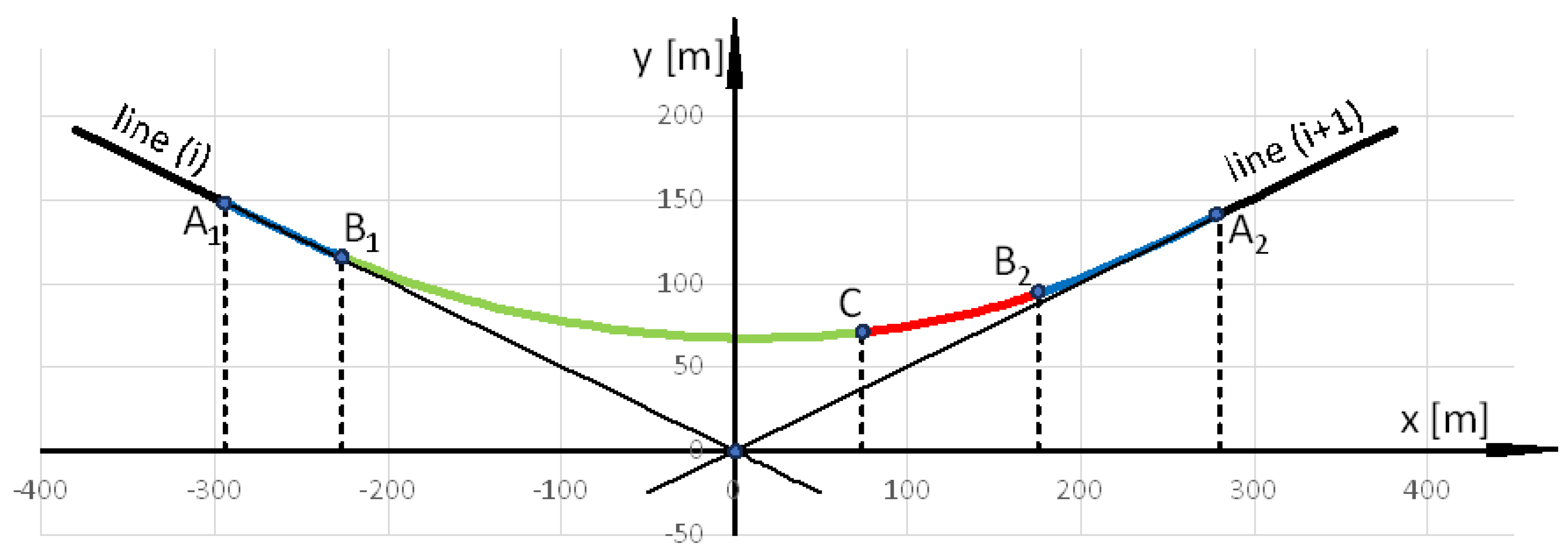
The length of the projection of the entire system on the abscissa axis was 574.208 m. Figure 10 shows the modeled geometric system in the local coordinate system. The green color indicates the circular arc CA1, the red color indicates the arc CA2, the blue color indicates the transition curves, and the purple color indicates the straight sections.

Figure 10.
Geometric system of the compound curve modeled using the analytical method in the local coordinate system.
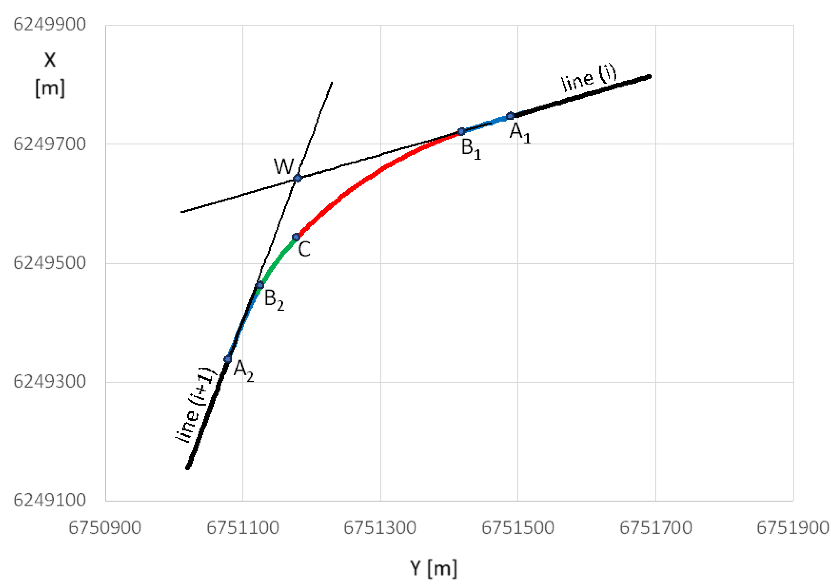
Finally, the obtained solution was transformed to the PL-2000 system, performing the reverse operation than was done when creating the LCS. Therefore, in the formulas used [34]
there is a negative value of the angle β. The final form of the geometric system is presented in Figure 11 (the colors of the markings are as in Figure 10).
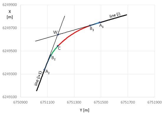
Figure 11.
Geometric system of the compound curve modeled using the analytical method in the PL-2000 system.
8. Conclusions
This article addresses the issue of designing classic compound curves, i.e., a geometric system consisting of two circular arcs of different radii, pointing in the same direction and connected directly to each other. Compound curves are currently used on tram lines; they also occur on railways, but new ones are not built there anymore. Therefore, in relation to railway lines, the aim is to obtain the possibility of reproducing (i.e., modeling) the existing geometric layout with compound curves, so that it is then possible to correct the horizontal ordinates in the area where the circular arches connect. For this purpose, it was necessary to develop an effective method for designing such a system, which, however, by assumption, will not be used to determine the coordinates of a new compound curves, but to model the existing system (with a view to its later modification).
To solve the problem, an analytical design method was used, in which the individual elements of these geometric systems are described by mathematical equations. The design itself is carried out in the appropriate local Cartesian coordinate system, the basis of which is the symmetrically set adjacent main directions of the route. The origin of the local coordinate system is located at the intersection point of the adjacent main directions, the coordinates of which in the global system are known.
In order to be able to operate in the local coordinate system, one must first perform an auxiliary procedure aimed at determining the basic computational quantities. These quantities refer to the regions of the geometric system connecting the ends of the extreme straight segments (i.e., the beginnings of the transition curves) with the connection point of both circular arcs. This refers to the lengths of the projections of transition curves and circular arcs on the horizontal and vertical axes.
The construction of a compound curve, i.e., the connection of the existing horizontal arcs with radii R1 and R2, is carried out in the auxiliary coordinate system and then transferred to the local coordinate system. The formulas for the coordinates of characteristic points are presented, in order to then finalize the design process by determining the course of the route sections located between these points. The obtained possibilities of modeling the compound curve are illustrated by the included calculation example.
Obtaining the possibility of reproducing (i.e., modeling) the existing geometric system with compound curves makes it possible to eliminate its critical place, which is the area where both circular arches connect. Further research on the discussed problem must go in this direction. The modification itself will consist in introducing appropriate transition curves between the connected arches, so that—based on the analysis—it is possible to recommend a curve for practical use.
Funding
This research received no external funding.
Institutional Review Board Statement
Not applicable.
Informed Consent Statement
Not applicable.
Data Availability Statement
The original contributions presented in this study are included in the article. Further inquiries can be directed to the author.
Conflicts of Interest
The author declares no conflicts of interest.
Abbreviations
The following abbreviations are used in this manuscript:
| PL-2000 | The Polish National Spatial Reference System |
| LCS | Local coordinate system |
| CA | Circular arc |
| TC | Transition curve |
References
- AutoCAD Civil 3D: Design, Engineering and Construction Software. Available online: http://www.autodesk.pl/products/civil-3d (accessed on 15 March 2025).
- Bentley Rail Track: Rail Infrastructure Design and Optimization. Available online: https://www.bentley.com/software/rail-design (accessed on 15 March 2025).
- Hodas, S. Design of railway track for speed and high-speed railways. Procedia Eng. 2014, 91, 256–261. [Google Scholar] [CrossRef]
- Soleymanifar, M.; Tavakol, M. Comparative study of geometric design regulations of railways based on standard optimization. In Proceedings of the 6th International Conference on Researches in Science and Engineering & 3rd International Congress on Civil, Architecture and Urbanism in Asia, Bangkok, Thailand, 9 September 2021. [Google Scholar]
- Aghastya, A.; Prihatanto, R.; Rachman, N.F.; Adi, W.T.; Astuti, S.W.; Wirawan, W.A. A new geometric planning approach for railroads based on satellite imagery. AIP Conf. Proc. 2023, 2671, 050005. [Google Scholar]
- Tasci, L.; Kuloglu, N. Investigation of a new transition curve. Balt. J. Road Bridge Eng. 2011, 6, 23–29. [Google Scholar] [CrossRef]
- Zboinski, K.; Woznica, P. Optimisation of polynomial railway transition curves of even degrees. Arch. Transp. 2015, 35, 71–86. [Google Scholar] [CrossRef]
- Kobryn, A. Universal solutions of transition curves. J. Surv. Eng. 2016, 142, 04016010. [Google Scholar] [CrossRef]
- Koc, W. New transition curve adapted to railway operational requirements. J. Surv. Eng. 2019, 145, 04019009. [Google Scholar] [CrossRef]
- Kobryn, A. Design of curvilinear sections in vertical alignment of roads and railways using general transition curves. Autom. Constr. 2024, 163, 105423. [Google Scholar] [CrossRef]
- Alfi, S.; Bruni, S. Mathematical modelling of train–turnout interaction. Veh. Sys. Dyn. 2009, 47, 551–574. [Google Scholar] [CrossRef]
- Bugarin, M.R.; Orro, A.; Novales, M. Geometry of high speed turnouts. Transp. Res. Rec. 2011, 2261, 64–72. [Google Scholar] [CrossRef]
- Palsson, B.A. Design of optimization of switch rails in railway turnouts. Veh. Sys. Dyn. 2013, 51, 1610–1639. [Google Scholar] [CrossRef]
- Ping, W. Design of high-speed railway turnouts. In Theory and Applications; Elsevier Science & Technology: Oxford, UK, 2015. [Google Scholar]
- Fellinger, M.; Marschnig, S.; Wilfling, P.A. Innovative track geometry data analysis for turnouts—Preparations to enable the turnout behaviour description. In Proceedings of the 12th World Congress on Railway Research: Railway Research to Enhance the Customer Experience, Tokyo, Japan, 28 October–1 November 2019. [Google Scholar]
- Koc, W. Analytical method of connecting parallel tracks located in a circular arc using curved turnouts. J. Transp. Eng. Part A Systems 2020, 146, 04019081. [Google Scholar] [CrossRef]
- Tonias, E.C.; Tonias, C.N. Compound and Reversed Curves. In Geometric Procedures for Civil Engineers; Springer International Publishing AG: Cham, Germany, 2016; pp. 185–242. [Google Scholar]
- Koc, W. Design of compound curves adapted to the satellite measurements. Arch. Transp. 2015, 35, 37–49. [Google Scholar] [CrossRef]
- Koc, W.; Specht, C. Application of the Polish active GNSS geodetic network for surveying and design of the railroad. In Proceedings of the First International Conference on Road and Rail Infrastructure—CETRA 2010, Univ. of Zagreb, Opatija, Croatia, 17–18 May 2010; pp. 757–762. [Google Scholar]
- Regulation of the Council of Ministers of 15 October 2012 on the National Spatial Reference System (In Polish). J. Laws 2012, pos. 1247. Available online: https://eli.gov.pl/eli/DU/2012/1247/ogl (accessed on 15 March 2025).
- Koc, W. Design of rail-track geometric systems by satellite measurement. J. Transp. Eng. 2012, 138, 113–122. [Google Scholar] [CrossRef]
- Koc, W. Analytical method of modelling the geometric system of communication route. Math. Probl. Eng. 2014, 2014, 679817. [Google Scholar] [CrossRef]
- Koc, W. The analytical design method of railway route’s main directions intersection area. Open Eng. 2016, 6, 1–9. [Google Scholar] [CrossRef]
- Koc, W. Identification of transition curves in vehicular roads and railways. Logist. Transp. 2015, 28, 31–42. [Google Scholar]
- Koc, W. Extending transition curve in analytical design method. Transp. Overview 2016, 71, 1–12. [Google Scholar] [CrossRef]
- Koc, W. Arching of railway turnouts by analytical design method. Curr. Appl. Sci. Technol. 2017, 25, CJAST.39093. [Google Scholar] [CrossRef]
- Koc, W. Shaping of the turnout diverging track with variable curvature sections. Int. J. Rail Transp. 2017, 5, 229–249. [Google Scholar] [CrossRef]
- Koc, W. Optimum shape of turnout diverging track with segments of variable curvature. J. Transp. Eng. Part A Syst. 2019, 145, 04018077. [Google Scholar] [CrossRef]
- Koc, W. Analytical design method for widening the intertrack space. Curr. Appl. Sci. Technol. 2019, 32, CJAST.46393. [Google Scholar] [CrossRef] [PubMed]
- Koc, W. The method of determining horizontal curvature in geometrical layouts of railway track with the use of moving chord. Arch. Civ. Eng. 2020, 66, 579–591. [Google Scholar]
- Koc, W. Estimation of the horizontal curvature of the railway track axis with the use of a moving chord based on geodetic measurements. J. Surv. Eng. 2022, 148, 04022007. [Google Scholar] [CrossRef]
- Koc, W. The procedure of identifying the geometrical layout of an exploited railway route based on the determined curvature of the track axis. Sensors 2023, 23, 274. [Google Scholar] [CrossRef]
- Koc, W. Determination of track axis coordinates in the analytical method of designing railway route geometry. Eur. J. Appl. Sci. 2024, 12, 339–362. [Google Scholar] [CrossRef]
- Korn, G.A.; Korn, T.M. Mathematical Handbook for Scientists and Engineers, 1st ed.; McGraw–Hill Book Company: New York, NY, USA, 1968. [Google Scholar]

Disclaimer/Publisher’s Note: The statements, opinions and data contained in all publications are solely those of the individual author(s) and contributor(s) and not of MDPI and/or the editor(s). MDPI and/or the editor(s) disclaim responsibility for any injury to people or property resulting from any ideas, methods, instructions or products referred to in the content. |
© 2025 by the author. Licensee MDPI, Basel, Switzerland. This article is an open access article distributed under the terms and conditions of the Creative Commons Attribution (CC BY) license (https://creativecommons.org/licenses/by/4.0/).