Analysis of Resampling Methods for the Red Edge Band of MSI/Sentinel-2A for Coffee Cultivation Monitoring

Abstract

Spectral indices such as NDRE (Normalized Difference Red Edge Index), CCCI (Canopy Chlorophyll Content Index), and IRECI (Inverted Red Edge Chlorophyll Index), derived from the Red Edge band of MSI/Sentinel-2A (B05, B06, B07), are critical for coffee monitoring. To align the Red Edge band (20 m resolution) with the NIR band (10 m resolution), the nearest neighbor, bilinear, cubic and Lanczos resampling methods were used, available in the Terra package in the R software(4.4.0). This study evaluates these methods using two original B05 images from 24 November 2023, and 21 September 2023, covering the “Ouro Verde” (15 ha) and “Canto do Rio” (45 ha) farms in Bahia, Brazil. A total of 500 random points were analyzed using PSF, linear models, and cross-validation with R², MAE, and RMSE. PSF analysis confirmed data integrity, and the cubic method demonstrated the best performance (R² = 0.996, MAE = 0.008 and RMSE = 0.012 in the “Ouro Verde” Farm and R² = 0.995, MAE = 0.007 and RMSE = 0.011 in the “Canto do Rio” Farm). The results highlight the importance of selecting appropriate resampling methods for precise remote sensing in coffee cultivation, ensuring accurate digital processing aligned with study objectives.

1. Introduction

Studies on remote sensing (RS) in coffee production have advanced in several countries, contributing to the improvement of production area management and increasing competitiveness in the global market [1,2].

This is especially important for Brazil, as the world’s largest producer and exporter of coffee beans, with 54.76 million 60 kg bags produced in 2024. In total, there are more than 330,000 coffee producers, 78% of whom are small-scale farmers, spread across approximately 1900 municipalities [3,4].

These advancements are due to the introduction of precision agriculture (PA), which refers to the use of geotechnologies for efficient, profitable, and sustainable rural management. When applied to coffee production, PA is referred to as precision coffee farming (PCF) [5,6].

Among these geotechnologies is orbital RS, conducted using satellite imagery. The applications of this technology range from identifying zones of productive potential and management areas, mapping and classifying areas, crop forecasting, and productivity estimation, to identifying diseases and pests, verifying leaf nitrogen content, and analyzing the spatial variability of crop attributes [7,8].

Several spectral indices are employed in remote coffee monitoring, particularly those incorporating the Red Edge spectral band, such as NDRE (Normalized Difference Red Edge Index), CCCI (Canopy Chlorophyll Content Index), and IRECI (Inverted Red Edge Chlorophyll Index) [9,10,11,12].

One of the main sources for obtaining these indices is the MSI (Multispectral Instrument) onboard Sentinel-2A, which includes three Red Edge bands (B05—Red Edge 1, B06—Red Edge 2, B07—Red Edge 3) captured at a 20 m spatial resolution [13]. To compute these indices, resampling is required to match the spatial resolution of the NIR band (10 m), a key reference in vegetation analysis. This process involves adjusting spatial resolution using interpolation methods such as nearest neighbor, bilinear, cubic, and Lanczos [14,15].

The characteristics and effects of these methods will be detailed in the Materials and Methods section. However, based on the characteristics of the methods, it is hypothesized that the nearest neighbor model might achieve good results, not because it is the most suitable model, but due to its characteristic of preserving the original image data.

Each of these interpolation methods has specific characteristics that define how spatial information is reconstructed. For instance, the nearest neighbor model preserves the pixel values, resulting in minimal alteration of the original data. However, in terms of RS coffee farming, bilinear interpolation has been applied to resample B05 band from 20 to 10 m resolution to evaluate the effects of hailstorms on Arabica coffee plantations using NDVI and NDRE indices [16].

This study employed the Semi-Automatic Classification (SPC) plugin in QGIS and concluded that NDRE is more sensitive than NDVI in demonstrating variations in vegetation index values across different Arabica coffee varieties. The same procedure was followed by other researchers [17]. Although the effects of these methods are well documented in the literature, they have been overlooked in studies on RS of coffee farming that utilize the Red Edge spectral band from the MSI/Sentinel-2, as well as in the validation of these methods, depending on the specific objectives of the resampling.

On the other hand, research on the topic has been conducted, including reviews of resampling methods applied to different types of images and their forms of quantitative and qualitative validation, both in hyperspectral and multispectral images, as is the case with the MSI/Sentinel-2 sensor [18]. Another study [19] has already shown that cubic interpolation is particularly effective for agricultural applications, where smooth transitions between pixel values are essential for accurate vegetation analysis. Similarly, it has also been observed [20] that the choice of resampling method can significantly impact the quality of spectral indices, especially when dealing with high-resolution data like those from Sentinel-2.

In addition to the resampling methods mentioned above, other procedures have been applied in RS studies, such as spline interpolation, Kriging, and convolutional neural networks (CNNs), which have shown promising results in various applications. For instance, spline interpolation has been effective in generating smooth surfaces with high geometric precision, which is particularly useful for capturing subtle spectral variations in agricultural monitoring [21]. Similarly, Kriging, a geostatistical method, has been applied to account for spatial autocorrelation in heterogeneous landscapes, such as coffee farms with varying growth stages [22]. On the other hand, CNNs have demonstrated superior performance in preserving fine details and reducing artifacts in resampled images, although they require significant computational resources and training data [23].

In this context, this technical note aims to test and validate different resampling methods for the Red Edge spectral band of the MSI/Sentinel-2, with the objective of obtaining indices for monitoring coffee farming and enhancing digital processing for this purpose. In this regard, this study contributes to the field by providing a systematic evaluation of resampling methods specifically for the Red Edge band of Sentinel-2, with a focus on coffee farming.

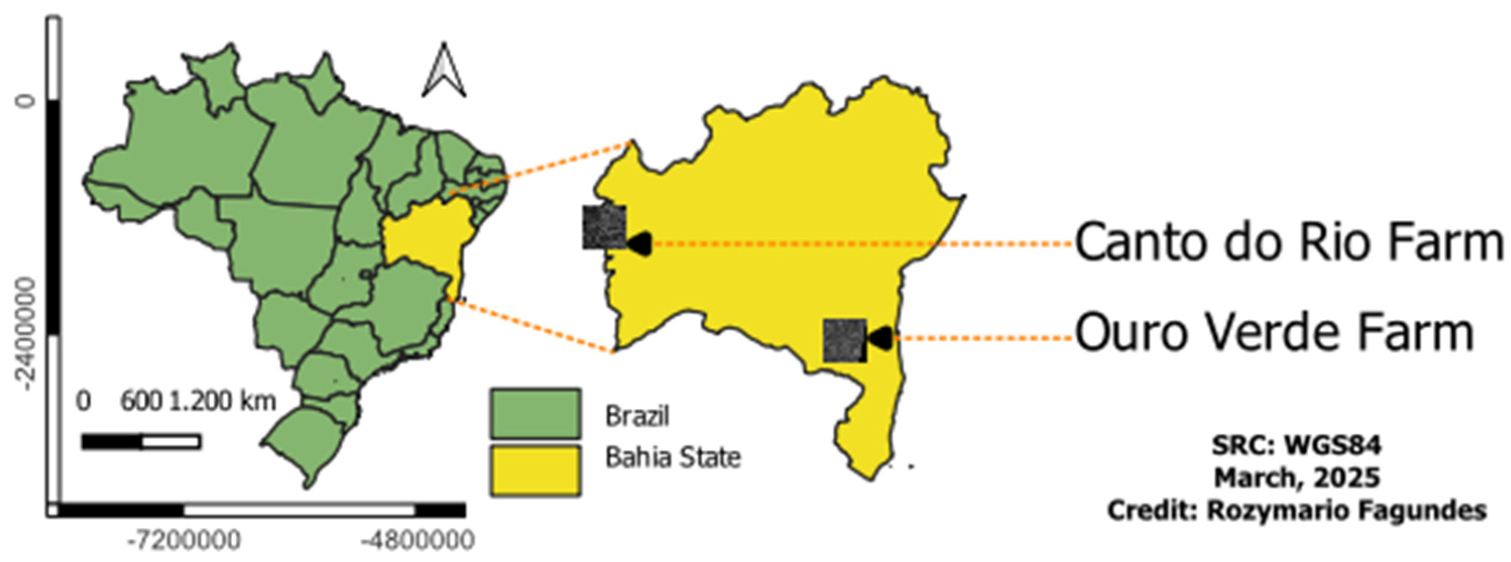
2. Materials and Methods

This study used images from the MSI (Multispectral Instrument) sensor on the Sentinel-2A satellite, which has 13 spectral bands, including three bands in the Red Edge range: 705 nm (B05), 740 nm (B06) and 783 nm (B07), all with a spatial resolution of 20 m. The spectral characteristics are detailed in

Table 1. Spectral band characteristics of MSI/Sentinel-2A: band number, spectral band, wavelength, and spatial resolution.

Band Number	Spectral Band	Wavelength (nm)	Spatial Resolution (m)
B01	Costal aerosol	443	60
B02	Blue	490	10
B03	Green	560	10
B04	Red	665	10
B05	Red Edge 1	705	20
B06	Red Edge 2	740	20
B07	Red Edge 3	783	20
B08	NIR	842	10
B8A	NIR narrow	865	20
B09	Water vapor	945	60
B10	Cirrus	1380	60
B11	SWIR 1	1910	60
B12	SWIR 2	2190	20

. The images used were obtained at the L2A processing level, already atmospherically corrected for surface reflectance, dispensing with additional correction steps.

The workflow comprises four main steps: (1) image acquisition and preparation; (2) generation of random sample points; (3) application of resampling methods and extraction of spectral values; and (4) statistical validation of the results. Two B05 band images with 0% cloud cover were selected, corresponding to Arabica coffee (Coffea arabica L.) production areas in the state of Bahia, Brazil: the “Ouro Verde” Farm (15 ha), located in Barra do Choça (southwest), and the “Canto do Rio” Farm (45 ha), in Luís Eduardo Magalhães (west), acquired on 24 November and 21 September 2023, respectively. Figure 1 shows the geographic locations of the corresponding B05 images.

Initially, 500 randomly distributed sampling points were generated within the geographic extent of the original B05 images. The spectral values at these points were extracted from both the original B05 image (20 m) and the resampled images (10 m), using the nearest neighbor, bilinear, cubic, cubic spline and Lanczos resampling methods, available in the terra package (version 4.4.0) of R. These resampling techniques were selected due to their wide application in remote sensing and their distinct interpolation properties, facilitating a complete evaluation of their effects on coffee crop monitoring. Figure 2 shows a detailed visualization of the processed images, and a supplementary location map of the farms provides spatial context for the study sites.

For each sample point, the native spectral values were compared with the corresponding resampled values. The extraction was performed directly on the sample points, not selecting a specific pixel among the four generated by the resampling, but rather considering the exact position of the point in both resolutions. The objective was to evaluate the spectral fidelity maintained or distorted by each interpolation technique. Alternative approaches, such as Kriging or deep-learning-based interpolation methods, were not considered in this study. The resampling process was applied uniformly to all images, using the same kernel size and interpolation window.

Table 2. Description of resampling methods and their effects.

Resampling Methods	Characteristics
Nearest Neighbor	Assigns the value of a pixel based on the nearest neighboring pixel, thereby preserving the original image data. However, this approach can lead to duplication of values, potential loss of fine details, and slight spatial misalignment, requiring careful application depending on the study’s objectives.
Bilinear	Determines a new pixel value by interpolating between the four nearest points, using a weighted averaging approach. This method provides smoother transitions between pixels but may introduce slight blurring effects.
Cubic	Computes the value of a new pixel by considering the 16 nearest neighbors, applying weighted averaging. This approach enhances image smoothness and reduces pixelation, albeit at a higher computational cost.
Lanczos	Uses a high-quality Lanczos kernel to interpolate signal values, effectively preserving image details while reducing aliasing effects. Although this method requires increased processing time, it generally yields superior visual and spectral quality in resampled images.

provides a comparative summary of the main attributes and differences between these methods [14,15].

Spatial analysis of the distribution patterns of the sample points was conducted using the spatstat package in R. The second-order spatial functions Ripley’s K, G function (distance to the nearest neighbor), and F function (distance from a random point to the nearest sample point) were applied.

These analyses were performed directly in geographic coordinates (WGS84 system); therefore, the parameter r was interpreted in decimal degrees. This precaution ensures consistency with the unit of measurement of the non-reprojected spatial data.

Recognizing that the random distribution of the points may include mixed pixels located at radiometric edges, the study adopted a conservative approach: the points were extracted randomly and broadly, without spectral or spatial filters. This choice represents a limitation, but it was maintained to preserve the heterogeneity of the analyzed scenario. To reduce possible spatial biases and rigorously assess the performance of the resampling methods, the extracted data were normalized and subjected to a validation strategy in two complementary stages:

(1)

Initial division into 70% for training and 30% for testing, applied to the normalized data set extracted from the sample points. This stage aimed to simulate a real prediction scenario, using a fraction of the data not observed in the training.

(2)

K-fold cross-validation (k = 5, with 5 repetitions), applied only to the training subset. This approach allowed for the adjustment and validation of the linear regression models with greater statistical robustness, minimizing the effect of random partitioning. The final results refer exclusively to the performance obtained on the test set (30%).

All statistical analyses were performed in R, using the packages caret (for modeling and cross-validation), metrics (for calculating metrics such as RMSE, MAE and R²), and ggplot2 (for visualization). The metrics used are defined as: Mean Absolute Error (MAE), Root Mean Square Error (RMSE) and Coefficient of Determination (R²).

MAE (Equation (1)) expresses the average of the absolute errors between the observed (original) and predicted (resampled) values, and is a direct metric of accuracy. RMSE (Equation (2)) calculates the mean squared error and penalizes larger errors more heavily, which makes it more sensitive to outliers. R² (Equation (3)) measures the proportion of the variability of the original data explained by the regression model. The lower the MAE and RMSE values, and the closer the R² value is to 1, the better the performance of the evaluated method [24].

The equations used are:

$$\mathrm{R}\mathrm{M}\mathrm{S}\mathrm{E}=\sqrt{{\displaystyle \frac{1}{n}}}{\sum }_{i=1}^n{(y_i-{\hat{\mathrm{y}}}_i)}^2$$

(1)

$$\mathrm{M}\mathrm{A}\mathrm{E}={\displaystyle \frac{1}{n}}\sum _{i=1}^n\left|{\mathit{y}}_{\mathit{i}}-{\hat{\mathrm{y}}}_{\mathit{i}}\right|$$

(2)

$${\mathrm{R}}^2=1-{\displaystyle \frac{\sum res}{\sum tot}}$$

(3)

where y_i represents the original value of the spectral index; ${\hat{\mathrm{y}}}_{\mathrm{i}}$ is the value resulting from the resampling; ȳ is the average of the original values; n is the number of points analyzed.

3. Results

After resampling in R, all output images had a 10 m spatial resolution, according to the methods used. Then, it followed for the evaluation of the sample points.

3.1. Results of the Family Health Program (FHP) Evaluation

3.1.1. “Ouro Verde” Farm

In the Ripley’s K function (

Table 3. Results Ripley’s K function.

	r	Theo	Border	Trans	iso
Min.	0	0 × 100	0 × 100	0 × 100	0 × 100
1st Qu	6.862 × 103	1.48 × 1011	1.47 × 1011	1.46 × 1011	1.46 × 1011
Median	1.3725 × 104	5.92 × 1011	6.01 × 1011	6.00 × 1011	5.98 × 1011
Mean	1.3725 × 104	7.90 × 1011	7.86 × 1011	7.90 × 1011	7.87 × 1011
3rd Qu	2.0588 × 104	1.33 × 1012	1.33 × 1012	1.33 × 1012	1.32 × 1012
Max	2.745 × 104	2.37 × 1012	2.33 × 1012	2.37 × 1012	2.36 × 1012

; Figure 3b), the density of points is measured as a function of distance r, with an assessment of clustering or dispersion. According to the data, the distance ranges from 0 to 27,450 decimal degrees in the WGS84 coordinate system, characterizing a wide scale that allows the identification of patterns at short and long distances.

Theoretically, density increases with distance, indicating a random pattern. The mean values (border, trans, iso), in turn, vary between 7.86 × 10¹¹ and 7.90 × 10¹¹, and are above the expected values at some scales. Regarding clustering, the maximum observed density ranged from 2.33 × 10¹² to 2.37 × 10¹², suggesting strong clustering at larger scales. There is a tendency for points to cluster at larger scales (r > 2.0 × 10⁴) and behave close to random at smaller scales.

In the G function (

Table 4. Results G function.

	r	Theo	Han	rs	km	Hazard	Theohaz
Min.	0	0.0000	0.0000	0.0000	0.0000	0.0000000	0.0000000
1st Qu	2350	0.5130	0.5175	0.5131	0.5134	0.0000000	0.0006124
Median	4700	0.9438	0.9353	0.9357	0.9300	0.0000000	0.0012248
Mean	4700	0.7383	0.7290	0.7278	0.7267	0.0006211	0.0012248
3rd Qu	7050	0.9985	10.000	10.000	10.000	0.0004483	0.0018371
Max	9400	10.000	10.000	10.000	10.000	0.0377538	0.0024495

; Figure 3c), we observe the proximity between points, with a highlight on local clusters. The data show that short distances r vary from 0 to 9400 decimal degrees, and that the means (~0.73) and medians (~0.93) are slightly below the theoretical value, indicating proximity between points at small scales (han, rs, km).

The mean value in hazard is almost 0, suggesting the absence of significant gaps. In the distribution, the median of 0.93 is close to the theoretical value (0.94), pointing to a tendency of slight or subtle local clustering at small scales.

Through the F function (

Table 5. Results F function.

	r	Theo	cs	Rs	km	Hazard	Theohaz
Min.	0	0.0000	0.0000	0.0000	0.0000	0.0000000	0.0000000
1st Qu	2359	0.5157	0.5254	0.5244	0.5226	0.0003114	0.0006147
Median	4718	0.9450	0.9542	0.9548	0.9541	0.0009524	0.0012294
Mean	4718	0.7345	0.7387	0.7390	0.7382	0.0009808	0.0012294
3rd Qu	7077	0.9985	0.9977	0.9978	0.9978	0.0012554	0.0018441
Max	9436	10.000	10.000	10.000	10.000	0.0064643	0.0024588

; Figure 3d), we can measure the distribution of the nearest points in the total space and verify if there is uniformity or dispersion. Regarding the values of (r), there is a variation between 0 and 9436 decimal degrees.

A linear growth can be observed, indicating uniformity. The mean values (cs, rs, km) at ~0.73 suggest a uniform distribution with denser local areas. In hazard, the mean value of almost 0 indicates the absence of large empty areas. In the distribution, the median of ~0.95 shows that the points are close to uniformity, but with variable local density.

3.1.2. “Canto do Rio” Farm

The results of the PSF evaluation of the Canto do Rio Farm were similar:

The values of r range from 0 to 27,450 decimal degrees in the WGS84 coordinate system, in the results Ripley’s K function (

Table 6. Results Ripley’s K function.

	r	Theo	Border	Trans	iso
Min.	0	0	0	0	0
1st Qu	6862	1.48 × 1011	1.47 × 1011	1.48 × 1011	1.48 × 1011
Median	13,725	5.92 × 1011	5.92 × 1011	5.88 × 1011	5.85 × 1011
Mean	13,725	7.90 × 1011	7.90 × 1011	7.89 × 1011	7.83 × 1011
3rd Qu	20,588	1.33 × 1012	1.33 × 1012	1.33 × 1012	1.32 × 1012
Max	27,450	2.37 × 1012	2.36 × 1012	2.38 × 1012	2.37 × 1012

; Figure 4b). In the observed average density (border, trans, iso), there is proximity to the theoretical density, but with some deviations, which may indicate slight clustering or dispersion tendencies at specific scales.

The maximum observed density (2.37 × 10¹²) exceeds the theoretical (7.90 × 10¹¹), indicating clustering at larger scales. Thus, it is possible to infer that the border, trans, and iso methods present similar values and consistent results. The points show tendencies of slight clustering at larger scales (r > 2.0 × 10⁴)), but close to the random pattern at smaller scales.

In the analysis of short distances, the values of r vary from 0 to 9400 decimal degrees, in the results G function (

Table 7. Results G function.

	r	Theo	Han	rs	km	Hazard	Theohaz
Min.	0	0.0000	0.0000	0.0000	0.0000	0.0000000	0.0000000
1st Qu	2350	0.5130	0.5088	0.5000	0.5003	0.0000000	0.0006124
Median	4700	0.9438	0.9451	0.9447	0.9412	0.0000000	0.0012248
Mean	4700	0.7383	0.7382	0.7368	0.7355	0.0006246	0.0012248
3rd Qu	7050	0.9985	10.000	10.000	10.000	0.0004799	0.0018371
Max	9400	10.000	10.000	10.000	10.000	0.0377538	0.0024495

; Figure 4c). The theoretical function increases linearly up to 1.0, which represents a random pattern. The average values of 0.73 in han, rs, and km are slightly below the expected, indicating greater proximity between points at smaller scales.

Regarding the median, the observed (0.94) is close to the theoretical (0.94), indicating a strong clustering of points, with slight proximity between short distances. There is a slight tendency of proximity at small scales, without forming highly dense patterns.

The results of the F function (

Table 8. Results F function.

	r	Theo	cs	rs	km	Hazard	Theohaz
Min.	0	0.0000	0.0000	0.0000	0.0000	0.000	0.0000000
1st Qu	2359	0.5157	0.5224	0.5197	0.5180	2.25 × 10−2	0.0006147
Median	4718	0.9450	0.9496	0.9469	0.9461	6.14 × 10−1	0.0012294
Mean	4718	0.7345	0.7363	0.7353	0.7344	8.43 × 10−1	0.0012294
3rd Qu	7077	0.9985	0.9998	0.9997	0.9994	1.15	0.0018441
Max	9436	10.000	10.000	10.000	0.9997	3.78	0.0024588

; Figure 4d) show a variation of r between 0 and 9436 decimal degrees. While the theoretical function grows up to 1.0, the observed (cs, rs, km) shows that average values (0.73) are slightly below the expected, with a more dispersed pattern in some areas.

Hazard values (minimum of 0.00078) and maximum (0.0032) indicate that there are a few significant empty areas. In the distribution, it is observed that the median (0.94) is almost identical to the theoretical (0.94).

The points are relatively uniform, but there are locally denser areas. In this context, it is possible to observe that the results of the two points samples follow similar patterns, with slight local clustering at G scales, strong clustering at larger scales (K), and overall uniformity at F. The main difference between the two samples is at G, which is more evident in the Ouro Verde farm sample.

3.2. Cross-Validation Results and Metrics Evaluation

The cross-validation test and metric evaluation confirmed the hypothesis regarding the nearest neighbor resampling method, with perfect results (R² = 1, MAE = 0, RMSE = 0) for both the Ouro Verde farm and Canto do Rio farm images. The other methods also yielded strong results, with slight variations between the two farms.

3.2.1. “Ouro Verde” Farm

For the Ouro Verde farm (Figure 5), the cubic method (a) performed best (R² = 0.995, MAE = 0.007, RMSE = 0.011), followed by the bilinear method (R² = 0.994, MAE = 0.008, RMSE = 0.013), Lanczos (R² = 0.994, MAE = 0.008, RMSE = 0.013), and cubic spline (R² = 0.991, MAE = 0.010, RMSE = 0.015).

3.2.2. “Canto do Rio” Farm

For the Canto do Rio farm (Figure 6), the cubic method also showed the highest performance (R² = 0.995, MAE = 0.007, RMSE = 0.011), followed by bilinear (R² = 0.994, MAE = 0.007, RMSE = 0.012), Lanczos (R² = 0.993, MAE = 0.008, RMSE = 0.013), and cubic spline (R² = 0.991, MAE = 0.009, RMSE = 0.015).

4. Discussion

The analysis of the results of the resampling methods revealed only minor variations among them in terms of accuracy, appearing to be generally reliable. Similar results were found in studies examining sugarcane crop classification and discrimination using MSI/Sentinel-2 imagery [14].

However, the authors highlight that simpler methods, such as bilinear and nearest neighbor, which require less processing time, may be preferable to more complex techniques, such as cubic and Lanczos, which demand more processing time. However, advancements in cloud processing can mitigate concerns about computational intensity.

Nearest neighbor, bilinear, and cubic methods have been widely applied in satellite image processing. For instance, Boggione and Costa [25] employed such methods for interpolating RapidEye and CBERS imagery, aiming to assess changes in grayscale values. They noted that resampling alters digital values (DVs) of the pixels in the output image, which in turn influences statistical results.

Similar effects were observed in a study using the Indian remote sensing (IRS) satellite images [26], which aimed to determine which resampling technique preserves the image quality the most, regarding mean absolute error and peak-to-noise ratio. Alterations in DVs were shown to be dependent on the original spatial resolution and specific image operations (scaling and rotation), emphasizing that resampling-induced changes are method- and context-dependent.

Additionally, mixed pixels and potential resampling artifacts introduced by interpolation methods were observed, particularly in areas with abrupt spectral transitions, such as field boundaries and vegetated regions. These factors must be considered when interpreting the results, as they could lead to unintended smoothing or spectral distortions.

Beyond traditional methods, resampling has been employed to generate high-resolution images from coarse-resolution satellite data. Lezine, Kyzivat, and Smith [27] explored the use of generative adversarial networks (GANs), comparing the results with cubic resampling for surface water mapping. Results suggested that GAN-based resampling can achieve comparable or superior performance to cubic resampling when high-resolution Planet CubeSat images were downscaled and subsequently resampled to their original resolution.

Resampling methods also address challenges such as spectral mixture discrimination, where multiple spectral features are captured within a single pixel. For example, in [28], a comparison of cubic convolution and nearest neighbor resampling on Landsat imagery found no statistically significant differences in the errors associated with pixel spectral response estimation, concluding that the results had no influence on using one method over another.

In the current study, the spectral mixture issue was more evident in areas with vegetation transitions, where interpolation methods influenced the spectral reflectance values, potentially altering vegetation index calculations. This highlights the need for caution when resampling spectral data for precision agriculture applications.

Another important application of resampling is upscaling imagery for various purposes. Guo et al. [29] explored the influence of spatial resolution on soil organic carbon (SOC) mapping using hyperspectral airborne imagery, upscaling the original 1 m resolution images by means of nearest neighbor, bilinear interpolation, and cubic convolution. Their study found that the use of different resampling methods has minor effects on the predictions of SOC against spatial resolution degradation.

While Lanczos resampling is less frequently used, likely due to its computational complexity, Madhukar and Narendra [30] evaluated Lanczos resampling alongside nearest neighbor and other methods for satellite remote sensing images, based on entropy, mean relative error, and execution time metrics.

They showed that Lanczos with a parameter achieved superior results, reducing aliasing, preserving sharpness, and minimizing ringing effects. These findings highlight the potential of Lanczos as a high-quality resampling option.

In summary, while all tested resampling methods showed minor differences in accuracy for this study, the impact of resampling on pixel values, particularly in the presence of mixed pixels and interpolation artifacts, should not be overlooked. These factors may affect subsequent spectral analyses and model predictions, emphasizing the need to balance computational efficiency with output quality when selecting a resampling method.

It is also important to highlight that, although the data used are specific to coffee crops, the methodological approach adopted, focused on the comparison between resampling methods applied to Red Edge images, can be generalized to other crops or applications in agricultural remote sensing, as long as the spectral and spatial conditions of the images are similar.

In addition, we recognize that resampling can significantly affect the calculation of derived spectral indices, such as NDRE, especially in areas with high intra-pixel variability. Resampling that smooths spectral transitions can attenuate extreme values or introduce artifacts, directly impacting agronomic analyses. Therefore, we suggest caution when applying these methods in operational contexts, recommending complementary analyses with NDRE and other spectral metrics as a future line of this work.

5. Conclusions

Red Edge band resampling for calculating indices such as NDRE, CCCI, and IRECI in coffee crop mapping can be performed using the terra package in R through nearest neighbor, bilinear, cubic, cubic spline, and Lanczos methods, which showed minimal differences in results.

However, the nearest neighbor method, while preserving original image data, may not be the most reliable for remote sensing of coffee crops. Based on the results, the cubic method proved to be the most suitable, followed by bilinear, Lanczos, and cubic spline.

Resampling influenced pixel DVs, affecting spectral responses and analyses. The extent of these changes varied by interpolation method, highlighting the need for careful selection based on study objectives. While no single method was deemed the best, considering DV modifications is crucial when choosing a resampling approach.

Future research can explore machine-learning-based resampling to enhance accuracy in coffee crop monitoring and evaluate method performance under different environmental conditions, refining remote sensing applications in precision agriculture.

References

1. De Castro, G.D.M.; Vilela, E.F.; de Faria, A.L.R.; Silva, R.A.; Ferreira, W.P.M. New vegetation index for monitoring coffee rust using sentinel-2 multispectral imagery. Coffee Sci. 2023, 18, e182170. [Google Scholar] [CrossRef]
2. Dias, G. Riscos Climáticos e Produtividade do Coffea Arabica L. Para as Principais Regiões Cafeeiras do BRASIL: Clima Presente e Futuro. Doctoral Thesis, Federal University of Itajubá, Itajubá, Brazil, 5 April 2024. [Google Scholar]
3. CONAB—Companhia Nacional de Abastecimento. Acompanhamento da Safra Brasileira de Café, v. 11 – Safra 2024, n.4- Quarto levantamento, Brasília, p. 1-53, Janeiro 2025. Available online: https://www.gov.br/conab/pt-br/atuacao/informacoes-agropecuarias/safras/safra-de-cafe/4o-levantamento-de-cafe-safra-2024/4o-levantamento-de-cafe-safra-2024 (accessed on 16 February 2025).
4. Campo e N. Anuário de Café 2021, 12th ed.; Editora Gazeta: Uberlândia, Brazil, 2021; ISSN 2316-6290. [Google Scholar]
5. Silva, F.M.; Alves, M.C. Cafeicultura de Precisão; Editora UFLA: Lavras, Brazil, 2013. [Google Scholar]
6. Ferraz, G.A.S. Cafeicultura de Precisão: Malhas Amostrais Para o Mapeamento de Atributos do Solo, da Planta e Recomendações. Ph.D. Thesis, Federal University of Lavras, Lavras, Brazil, 2012. [Google Scholar]
7. Santana, L.S.; Ferraz, G.A.S.; Santos, S.A.d.o.s.; Dias, J.E.L. Precision coffee growing: A review. Coffee Sci. 2022, 17, e172007. [Google Scholar] [CrossRef]
8. Melos, N.D. Uso de Análise Multivariada Para Identificação de Zonas de Potenciais Produtivos Agrícolas. Master’s Thesis, University of Santa Maria, Santa Maria, Brazil, 9 March 2023. [Google Scholar]
9. Barnes, E.M.; Clarke, T.R.; Richards, S.E.; Colaizzi, P.D.; Haberland, J.; Kostrzewski, M.; Waller, P.; Choi, C.; Riley, E.; Thompson, T.; et al. Coincident detection of crop water stress, nitrogen status and canopy density using ground-based multispectral data. In Proceedings of the 5th International Conference on Precision Agriculture, Bloomington, MN, USA, 16–19 July 2000. [Google Scholar]
10. Frampton, W.J.; Dash, J.; Watmough, G.; Milton, E.J. Evaluating the capabilities of Sentinel-2 for quantitative estimation of biophysical variables in vegetation. ISPRS J. Photogramm. Remote Sens. 2013, 82, 83–92. [Google Scholar] [CrossRef]
11. Chemura, A.; Mutanga, O.; Odindi, J.; Kutywayo, D. Mapping spatial variability of foliar nitrogen in coffee (Coffea arabica L.) plantations with multispectral Sentinel-2 MSI data. ISPRS J. Photogramm. Remote Sens. 2018, 138, 1–11. [Google Scholar] [CrossRef]
12. Nogueira, M.R.; de Carvalho Pinto, F.d.A.; Marçal de Queiroz, D.; Magalhães Valente, D.S.; Fim Rosas, J.T. A Novel Vegetation Index for Coffee Ripeness Monitoring Using Aerial Imagery. Remote Sens. 2021, 13, 263. [Google Scholar] [CrossRef]
13. ESA-Europe Spatial Agence. Sentinel Online. Available online: https://sentinels.copernicus.eu/web/sentinel/home (accessed on 12 December 2024).
14. Kai, P.M.; de Oliveira, B.M.; Vieira, G.S.; Soares, F.; Costa, R.M. Effects of resampling image methods in sugarcane classification and the potential use of vegetation indices related to chlorophyll. In Proceedings of the 2021 IEEE 45th Annual Computers, Software, and Applications Conference (COMPSAC), Madrid, Spain, 12–16 July 2021; pp. 1526–1531. [Google Scholar] [CrossRef]
15. Richards, J.A.; Richards, J. Remote Sensing Digital Image Analysis; Springer: Berlin/Heidelberg, Germany, 1999; Volume 3. [Google Scholar]
16. Rodrigues, S.A.; Cortez, J.W.; Henriques, H.J.R. Efeito da chuva de granizo em variedades do café arábica por meio de índices de vegetação. Agrarian 2021, 14, 433–441. [Google Scholar] [CrossRef]
17. Feio, S. Análise Multitemporal de Imagens de Satélite Sentinel-2 Como Suporte à Elegibilidade das Ajudas Comunitárias Agrícolas. Master’s Dissertation, University of Lisbon, Lisbon, Portugal, 2017. [Google Scholar]
18. Mookambiga, A.; Gomathi, V. Comprehensive review on fusion techniques for spatial information enhancement in hyperspectral imagery. Multidimens. Syst. Signal Process. 2016, 27, 863–889. [Google Scholar] [CrossRef]
19. Sadeghi, S.; Guo, L.; Toliyat, H.A.; Parsa, L. Wide Operational Speed Range of Five-Phase Permanent Magnet Machines by Using Different Stator Winding Configurations. IEEE Trans. Ind. Electron. 2012, 59, 2621–2631. [Google Scholar] [CrossRef]
20. Li, J.; Heap, A.D. A review of comparative studies of spatial interpolation methods in environmental sciences: Performance and impact factors. Ecol. Inform. 2011, 6, 228–241. [Google Scholar] [CrossRef]
21. Wahba, G. Spline Models for Observational Data; SIAM: Pennsylvania, PA, USA, 1990. [Google Scholar]
22. Oliver, M.A.; Webster, R. Kriging: A Method of Interpolation for Geographical Information Systems. Int. J. Geogr. Inf. Syst. 2014, 4, 313–332. [Google Scholar] [CrossRef]
23. Dong, C.; Loy, C.C.; He, K.; Tang, X. Image Super-Resolution Using Deep Convolutional Networks. IEEE Trans. Pattern Anal. Mach. Intell. 2016, 38, 295–307. [Google Scholar] [CrossRef] [PubMed]
24. James, G.; Witten, D.; Hastie, T.; Tibshirani, R. An Introduction to Statistical Learning: With Applications in R; Springer: Berlin/Heidelberg, Germany, 2013. [Google Scholar] [CrossRef]
25. Boggione, G.A.; Costa, D.D. Reamostragem em imagens de sensoriamento remoto: Uma abordagem sob o ponto de vista do maup. In Proceedings of the IV Simpósio Brasileiro de Geomática–SBG2017 I I, Presidente Prudente, São Paulo, Brazil, 24–26 July 2017; pp. 315–322, ISSN 1981-6251. [Google Scholar]
26. Porwal, S.; Katiyar, S.K. Performance Evaluation of Various Resampling Techniques on IRS Imagery. In Proceedings of the 2014 Seventh International Conference on Contemporary Computing (IC3), Noida, India, 9 August 2014. [Google Scholar] [CrossRef]
27. Lezine, E.M.D.; Kyzivat, E.D.; Smith, L.C. Super-Resolution Surface Water Mapping on the Canadian Shield Using Planet CubeSat Images and a Generative Adversarial Network. Can. J. Remote Sens. 2021, 47, 261–275. [Google Scholar] [CrossRef]
28. Ceccato, G.Z.; Das, N.; José, M.G.; Cesar, J. Avaliação dos valores de erro do modelo linear de mistura espectral em imagens etm+/landsat 7 a partir de reamostragens pelo vizinho mais próximo e convolução cúbica. Geociências 2021, 40, 795–810. [Google Scholar] [CrossRef]
29. Guo, L.; Shi, T.; Linderman, M.; Chen, Y.; Zhang, H.; Fu, P. Exploring the Influence of Spatial Resolution on the Digital Mapping of Soil Organic Carbon by Airborne Hyperspectral VNIR Imaging. Remote Sens. 2019, 11, 1032. [Google Scholar] [CrossRef]
30. Madhukar, B.N.; Narendra, R. Lanczos Resampling for the Digital Processing of Remotely Sensed Images. Lect. Notes Electr. Eng. 2013, 258, 403–411. [Google Scholar] [CrossRef]
Figure 1. In this figure, we see the map of Brazil, the map of the Bahia State, and the location of the satellite images corresponding to the “Canto do Rio” and “Ouro Verde” farms.
Geomatics 05 00019 g001
Figure 2. These are original images from the B05 band and the rural properties used as reference: (a) Image of the “Ouro Verde” Farm; (b) Image of the “Canto do Rio” Farm.
Geomatics 05 00019 g002
Figure 3. (a) Random sample points; (b) Ripley’s K function; (c) G function; (d) F function.
Geomatics 05 00019 g003aGeomatics 05 00019 g003b
Figure 4. (a) Random sample points; (b) Ripley’s K function; (c) G function; (d) F function.
Geomatics 05 00019 g004aGeomatics 05 00019 g004b
Figure 5. (a) Original image x cubic; (b) Original image x bilinear; (c) Original image x Lanczos; (d) Original image x cubic spline; (e) Original image x nearest neighbor.
Geomatics 05 00019 g005aGeomatics 05 00019 g005b
Figure 6. (a) Original image x cubic; (b) Original image x bilinear; (c) Original image x Lanczos; (d) Original image x cubic spline; (e) Original image x nearest neighbor.
Geomatics 05 00019 g006aGeomatics 05 00019 g006b