Article

Determining the Spectral Characteristics of Fynbos Wetland Vegetation Species Using Unmanned Aerial Vehicle Data

by
Kevin Musungu
1,2,*,
Moreblessings Shoko
1 and
Julian Smit
2
1
Department of Architecture, Planning and Geomatics, University of Cape Town, Cape Town 7700, South Africa
2
Department of Civil Engineering and Geomatics, Cape Peninsula University of Technology, Cape Town 8000, South Africa
*
Author to whom correspondence should be addressed.
Geomatics 2025, 5(2), 17; https://doi.org/10.3390/geomatics5020017
Submission received: 21 January 2025 / Revised: 24 April 2025 / Accepted: 24 April 2025 / Published: 29 April 2025

Abstract

:
The Cape Floristic Region (CFR) boasts rich biodiversity but faces threats from invasive species and land-use changes. Fynbos wetland vegetation within the CFR is under-mapped despite its crucial role in supporting biodiversity and maintaining hydrological cycles. This study assessed the potential of UAV VIS-NIR data, gathered during Spring and Summer, to identify the spectral characteristics of eleven Fynbos wetland species in a seep wetland. Spectral distances derived from reflectance data revealed distinct spectral clustering of plant species, highlighting which species could be distinguished from each other. UAV data also captured differences in reflectance across spectral bands for both dates. Spectral statistics indicated that certain species could be more accurately classified in Spring than in Summer, and vice versa. These findings underscore the efficacy of UAV multispectral data in analyzing the reflectance patterns of fynbos wetland species. Additionally, the sensitivity of UAV multispectral data to foliar pigment composition across different seasonal stages was confirmed. Lastly, species classification results demonstrated that a random forest classifier is well suited, with relative producer and user accuracies aligning with the derived spectral distances. The results highlight the potential of UAV imagery for monitoring these endemic species and creating opportunities for scalable mapping of Fynbos seep wetlands.

1. Introduction

The CFR contributes substantially to the local economy through fishing, flower harvesting, and tourism, contributing billions of Rands [1,2]. The Cape Fynbos, situated in the Cape Floristic Region (CFR) in South Africa, has rich floral diversity characterized by more than 8500 plant species, with more than 70% of these endemic to the Western Cape and Eastern Cape provinces in South Africa [3]. The Cape Peninsula, located South of Cape Town, has the greatest concentration of plant species in the CFR [4,5]. For instance, the Kogelberg region in the peninsula is called ‘the heart of the fynbos’ with more than 1650 plant species and the most significant floral diversity per unit area in the world [6]. The competing demands of economic growth from the floristic region and conservation efforts must be managed carefully [7,8,9] because the Fynbos Biome is more infested by invasive alien species than any other South African Biome [10,11]. Conservation efforts in the CFR must therefore be backed by updated information about the local vegetation [12,13].
Wetlands are vital because of their extensive biodiversity and essential role in hydrological and biogeochemical cycles [14,15]. Yet, the methods used to map terrestrial vegetation may be less effective for mapping wetland vegetation. The reason is that the reflectance spectra of wetland plants are influenced by underlying water and moist soil [16], and wetland species’ spectral signatures can vary significantly even within phenological seasons [17,18]. Moreover, environmental differences within wetlands can result in ecological patches that are sometimes smaller than satellite spatial footprints [19,20].
UAVs offer a solution to the limitations caused by the spatial resolution of satellite data. Their high-resolution data may also provide insights for new satellite sensors [21,22]. UAVs are also advantageous for their ability to deliver up-to-date data and efficiently map wetlands faster, more cost-effectively, and with minimal intrusion compared to traditional fieldwork methods [23,24]. Their superiority lies in their ability to provide very high-resolution aerial photographs and accommodate interchangeable payloads that can be used with diverse sensors [25,26]. Although their use is limited by proximity to the target site, UAVs hold significant potential for identifying Fynbos wetland plant species—a possibility that warrants further exploration.
Several studies have explored the potential of diverse remote sensing datasets as tools for sustainable mapping of vegetation in CFR. Studies have concentrated on a broad range of issues, including conservation efforts and the impact of surrounding land use on vegetation in this region [3,27,28,29]. Other areas of research include analysis of the impact of fires [30,31,32], understanding plant–water variables [33,34], habitat loss [35], detection of groundwater-dependent vegetation [22], detection of invasive alien vegetation [36,37,38,39], and delineating wetland ecotones [40]. However, there are a limited number of studies that employ UAVs or articulate plant species identification in wetlands within the Cape Floristic Region (CFR). This research is therefore crucial to conservation efforts, as many Fynbos species require hydric habitats [41]. Against the backdrop of this research gap, this study investigates UAV-based procedures for identifying the spectral traits of Fynbos plant species in inland seep wetlands.
The main objective of this study is to assess the effectiveness of UAV multispectral data in distinguishing wetland species, evaluating its efficacy in seasonal spectral changes, and analyzing its potential for species classification using machine learning.

2. Materials and Methods
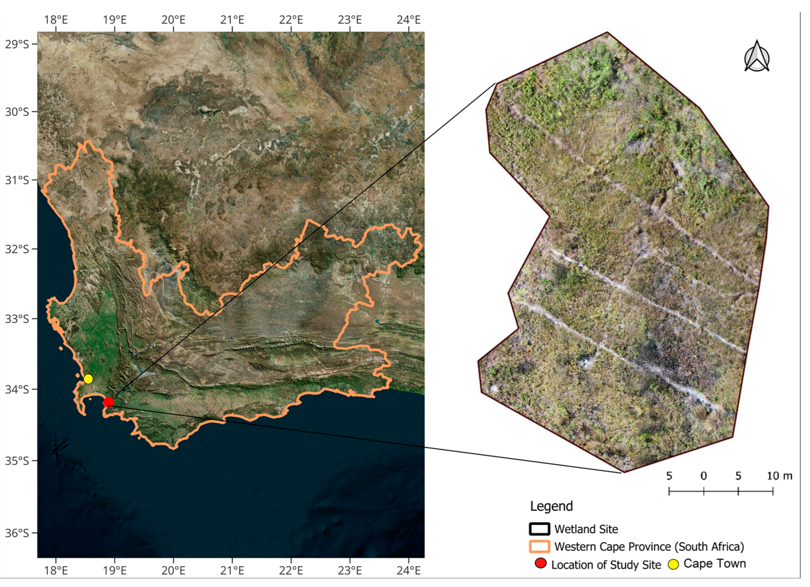
2.1. Study Area

The study site is part of the Kogelberg Sandstone Fynbos area, a part of the Western Cape province, in South Africa, which includes approximately 8486.778 Hectares of land owned by the municipality of Cape Town. The study area is located 80 km from Cape Town, just south of the upper Steenbras dam in the Steenbras Nature Reserve at geographical coordinates 34°10′53.5″ S and 18°54′23.8″ E. The region receives 80% of its yearly rainfall from April to September, and the dry seasons are typically from November to March [42,43]. The portions of the wetland at lower altitudes are permanently inundated, whilst those at higher elevations are seasonally saturated.

2.2. Identifying the Dominant Plant Species

A municipal dataset of vegetation plots depicting data along the three transect lines (see Figure 1) and the corresponding plot coordinates was used to identify the positions of spatially dominant plant species in the wetland. These plots also helped the researchers visually identify the appearance of the dominant wetland species, enabling the survey of ground truth positions for these species. Eleven spatially dominant wetland plant species comprising the Cyperaceae, Bruniaceae, Ericaceae, Grubbiaceae, Iridaceae, Proteaceae, and Restionaceae Fynbos families were identified. Table 1 lists their information. Figure 2 shows the appearance of plant species.

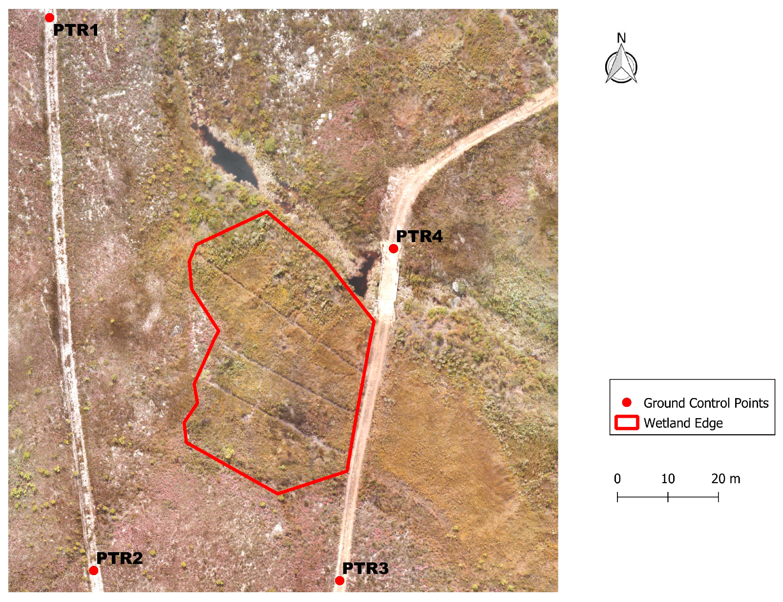
2.3. Creating Photogrammetric Ground Control Points

Five Ground Control Points (GCPs) consisting of permanent 12 mm round iron pegs were placed around the periphery of the study area. Placing GCPs around the study area enhances the positional and geometric accuracy in the orthomosaics [44,45]. The GCPs were coordinated using a Trimble R4 GNSS RTK System comprising a base, rover, and Trimble Juno data collectors [46]. The coordinates of the GNSS base station were determined using a three-hour static observation, and a Real-Time Kinematic (RTK) survey was undertaken to establish the coordinates of the four GCPs (PTR1–PTR4) around the wetland.

2.4. Acquiring UAV Data

The next step in the fieldwork involved capturing high-resolution aerial photography at the study site. A Parrot Sequoia (AgEagle Aerial Systems, Wichita, KS, USA) mounted on a DJI Phantom 3 quadcopter (DJI, Shenzhen, China) was used for the aerial survey of the wetland. Ground control targets were placed over the GCPs so that the centre of each target coincided with the surveyed point. The targets were plastic, white, and black, 1 m by 1 m wide, as per a similar study in the same area [46].
The flight height was 25 m above ground, with an 80% side lap and forward overlap and a flight speed of 5 m/s [46]. Figure 3 shows the layout of the GCPs and Table 2 shows the flight dates, times, and seasons. The low flying altitude results in high-resolution photographs and reduces atmospheric influence [47]. Moreover, the flying height was high enough to avoid downdraft disturbance on the vegetation. Additionally, the considerable overlap between the aerial photographs ensured that the GCPs were visible in several photos [48].
The Parrot Sequoia photos were calibrated using calibration panels and irradiance sensors. Before and after the flight mission, the drone was positioned approximately one metre above the calibration panel to capture three sets of photos with each multispectral sensor. The wavelength and the published mean scale factors of the Parrot Sequoia are shown in Table 3.

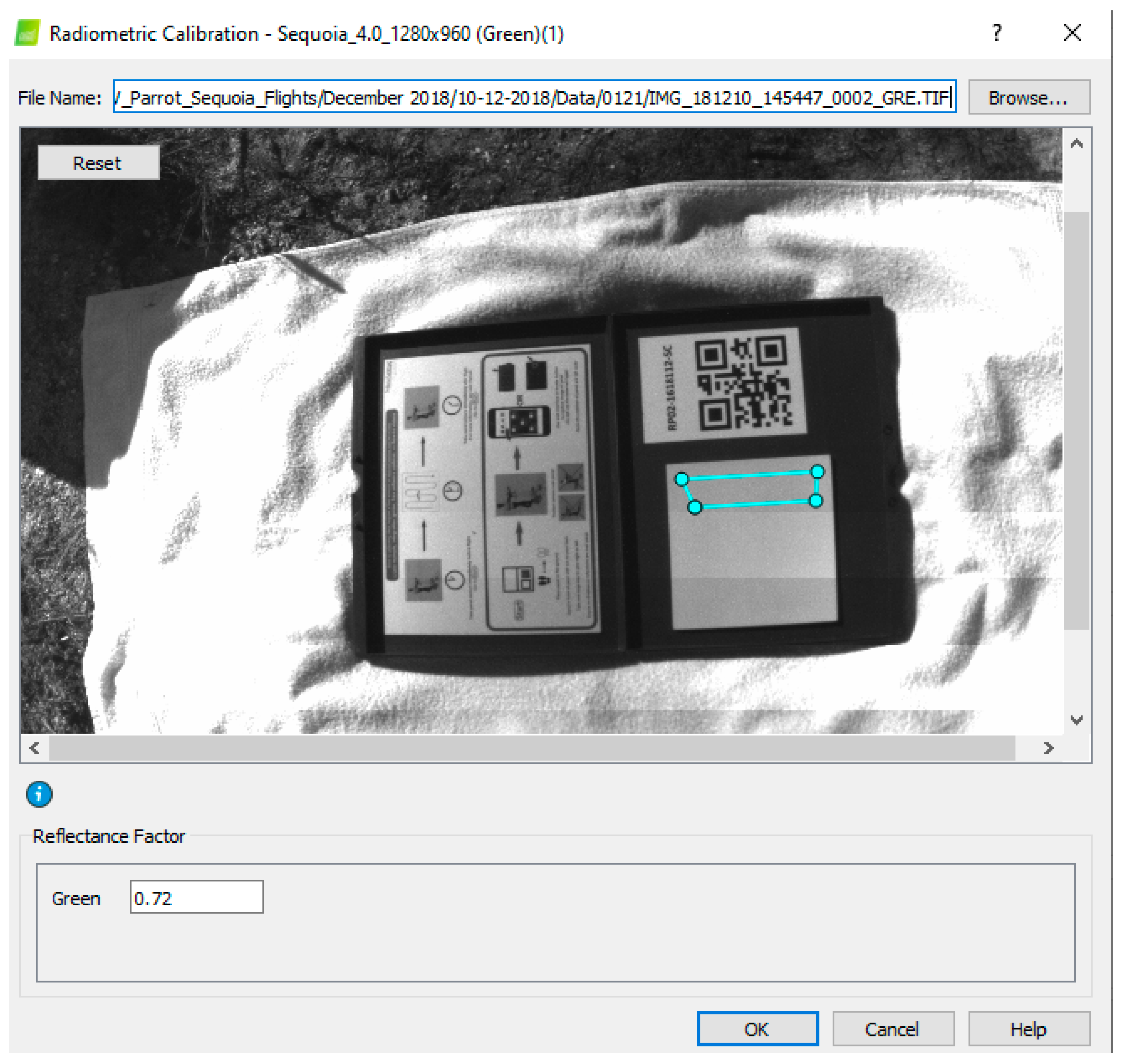
2.5. Processing UAV Data

The first step involved geometric calibration of the UAV data. UAV aerial photography contains geometric distortion due to lens distortions, sensor misalignment, terrain effects, changes in sampling rates, unstable platforms, and many more [49]. Known ground truth coordinates, obtained from Ground Control Points (GCPs), were used to develop polynomial equations and transform distorted dataset coordinates to the correct spatial locations [50,51]. An accurate Digital Elevation Model (DEM) is used to produce orthorectified images [49,52]. This study used a self-calibration bundle block adjustment based on the image data, structure from motion (SfM), and GCPs [53,54,55].
Firstly, 10,000 tie points were computed on the images to create a sparse point cloud and determine the camera pose. The geometric calibration of the sparse point cloud was based on the processed GNSS coordinates of the surveyed GCPs. The point cloud was georeferenced and transformed from the World Geodetic System 1984 (WGS84) coordinate system to the South African Hartebeesthoek94 coordinate system. The project heights were also constrained to the South African Geoid (SAGEOID 2010) to ensure interoperability with other local spatial datasets, such as the vegetation plots. Finally, a bundle adjustment was performed, and a high-resolution Digital Surface Model (DSM) was created (approximately 12-centimetre resolution) and used to generate high-resolution orthophotos and orthomosaics (approximately 3 cm resolution).
The second step was the radiometric correction. Radiometric calibration in UAV studies can be broadly categorized into two groups: those using calibration targets [56,57,58] and those using irradiance sensors [59,60,61]. Studies using calibration targets typically capture photographs of radiometric calibration targets before and after flight campaigns or place several radiometric reference targets (RRT) in the scene so that at least one is captured in each aerial photo. Then, an empirical line regression is calculated between the digital numbers of the reflectance panels and their known reflectance, which is used to convert the digital numbers in the photographs to at-surface reflectance [48,61].
The radiometric correction was performed in Pix4D Mapper (Pix4D, Lausanne, Switzerland, version 4.5). Reflectance was calculated using the average reflectance factor values provided with the camera calibration reflectance panels, sun irradiance information imported from the Camera Irradiance EXIF tag, and the calibration photos of the reflectance panels taken before and after the flights. The three sets of calibration photos were imported into Pix4D Mapper, and the published reflectance factors were inserted for each reflectance calibration photo (See Figure 4).
The atmospheric influence is negligible in UAV data gathered at low flight altitudes [49] with studies suggesting threshold altitudes of 60 m [62] to 100 m [47,63]. Also, because UAV flights are very short, the effects of variability in solar altitude, azimuth angles, and solar radiation during data capture on small sites are commonly presumed negligible [61].

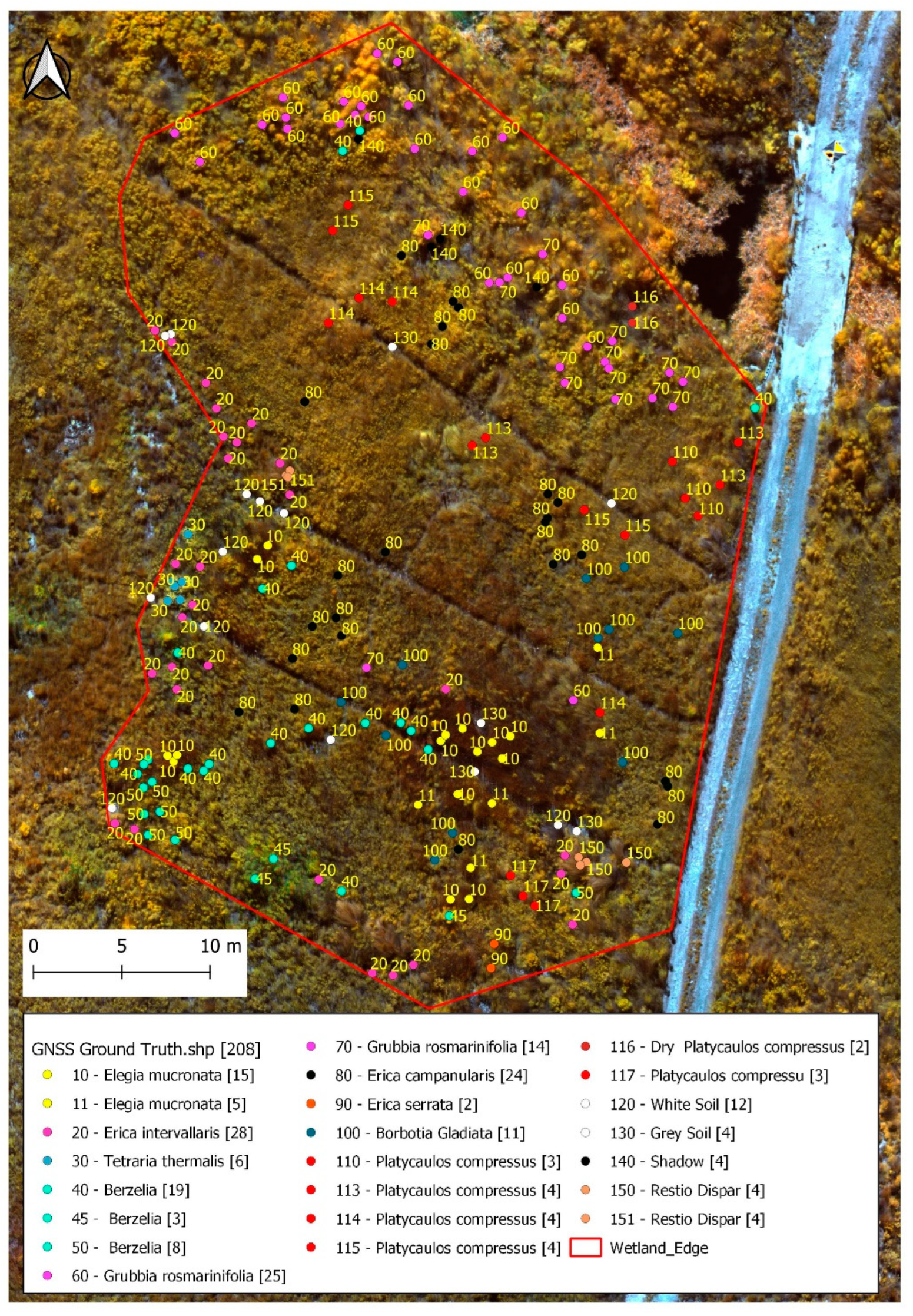
2.6. Processing Ground Truth Data and Spectral Curves

The processed orthomosaics corresponding to the different camera spectral bands were layer-stacked using Quantum GIS (QGIS version 3.22). During the survey of the GCPs, 208 ground truth points, locations, and species at that location were identified based on archival transect data and a field trip with a botanist. Homogenous clusters were surveyed using GNSS within the wetland (Figure 5). A shapefile was created from the coordinates of the surveyed points and imported into a GIS. Then, another 257 polygons of specific fynbos species were digitized in the GIS for classifier training and validation. The polygons were identified by their similarity to the species at the locations of the overlaid surveyed points. A Stratified Proportional Random Sampling (SPRS) was used to ensure each vegetation type was adequately represented, improving the overall mapping and monitoring of species [64]. The point-in-polygon GIS algorithm was used to randomly create new points within the polygons such that each polygon could accommodate up to 40 points, each overlaying a unique pixel, based on the pixel resolution of the orthomosaics. The new points layer and ground truth points, totaling 8889 points, were used to sample reflectance values where they intersected with the orthomosaics of the spectral bands. As a result, the point shapefile contained attribute data consisting of the land cover classes and corresponding reflectance values in the spectral bands. The data were exported to a spreadsheet and analyzed using R software (version 4.2.1). The spectral reflectance values for each band were averaged separately for each land cover class using the “dplyr” library in R software. Then, each species’ averaged spectral reflectance values were plotted against the corresponding band’s central wavelength.
In addition, Euclidean spectral distances were computed to investigate similarity in reflectance across species [65,66,67], and quantile–quantile (Q-Q) plots were plotted to investigate normality. Since the data showed skewness, a non-parametric pairwise Wilcox test [68] was computed for each pair of plant species across wavelengths for both data collection dates. The computations were performed using “dplyr”, “tidyr”, and “stats” libraries, and the visualizations were generated using the “pheatmap” and “ggplot2” libraries in R Software (version 4.2.1). The corresponding p-values (p < 0.05) indicated the likelihood that the observed variance between group means occurred by chance [69]. A p-value below 0.05 is typically considered statistically significant [70].

2.7. Classification of the Wetland Species

Several classification algorithms were used in the study. The decision on what classifier to utilize was informed by previous review studies that focused on delineating plant species and vegetation classification studies [71,72,73]. Other considerations included the capacity of the classifier to handle the notable uneven spatial distribution of the plant species within the study area. Consequently, the classifiers investigated were Random Forests, K-Nearest Neighbour, and Support Vector Machines [74,75]. These classifiers represent several groups of ML algorithms, namely logic-based algorithms (RF), instance-based learning (KNN), and Support Vector Machines [76]. RF combines the prediction of several decision trees based on multiple subsets of training data, making it robust to overfitting even with high-dimensional data [77]. SVMs can derive optimal hyperplanes in multi-dimensional classification with the highest margin between classes [78,79], and KNN is robust to noisy data [79]. All these classifiers have been used extensively in recent studies.
As per multiple studies, some of the sample data were retained to validate the classification [80,81,82]. Seventy per cent of the samples were used for supervised pixel-based classification with optimized hyperparameters, and the rest for validation. The accuracy statistics of the classification were calculated using the retained validation samples (30%). This was achieved using the Semi-Automatic Classification Plugin (SCP) in QGIS and the r.kappa function in GRASS GIS. The additional spectral information derived from indices improved the classification results. The validation of the classification was performed using kappa, overall, and per-class producer and user accuracy metrics [80,82]. The methodology is summarized in Figure 6.

3. Results and Discussion

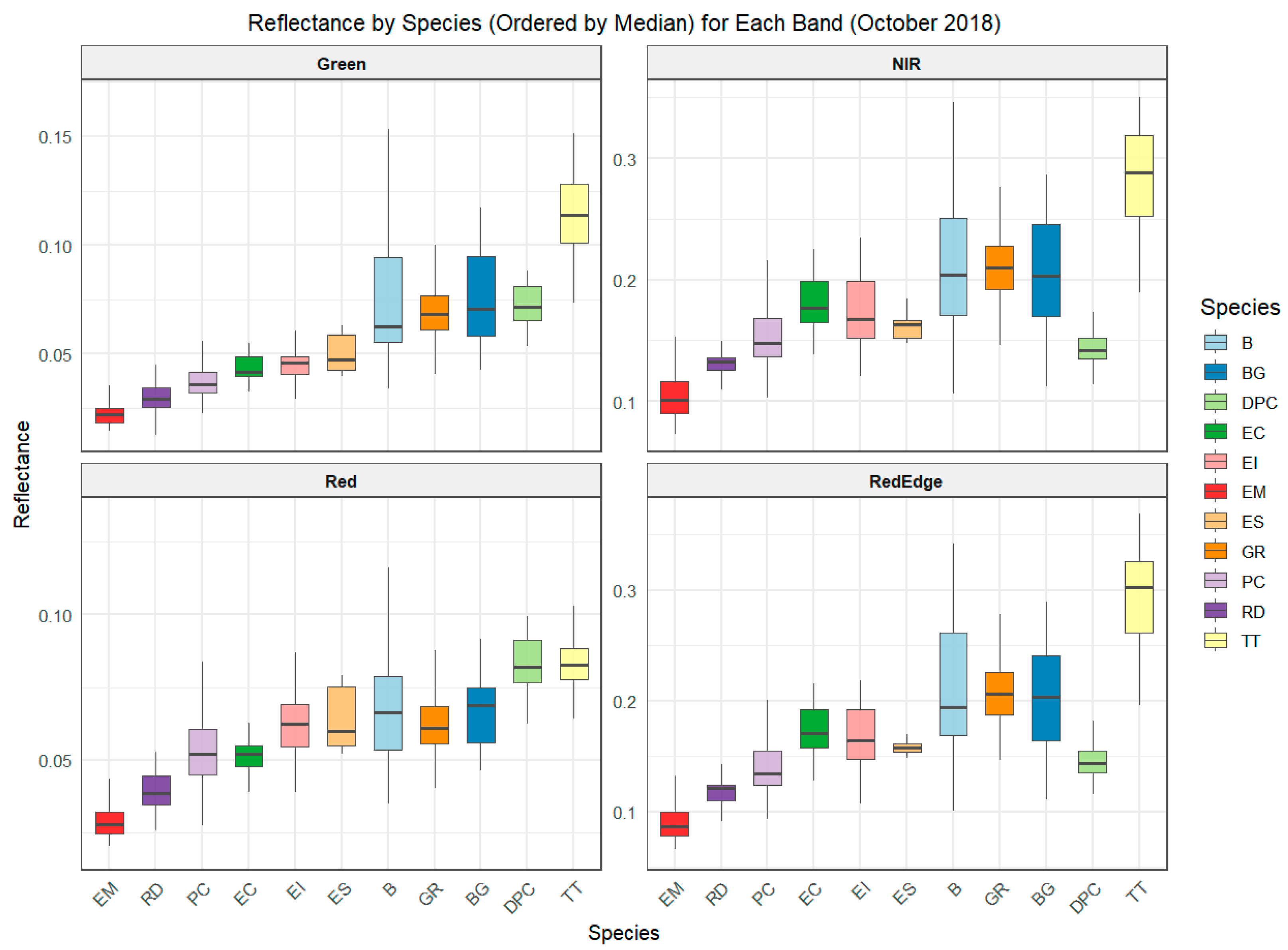
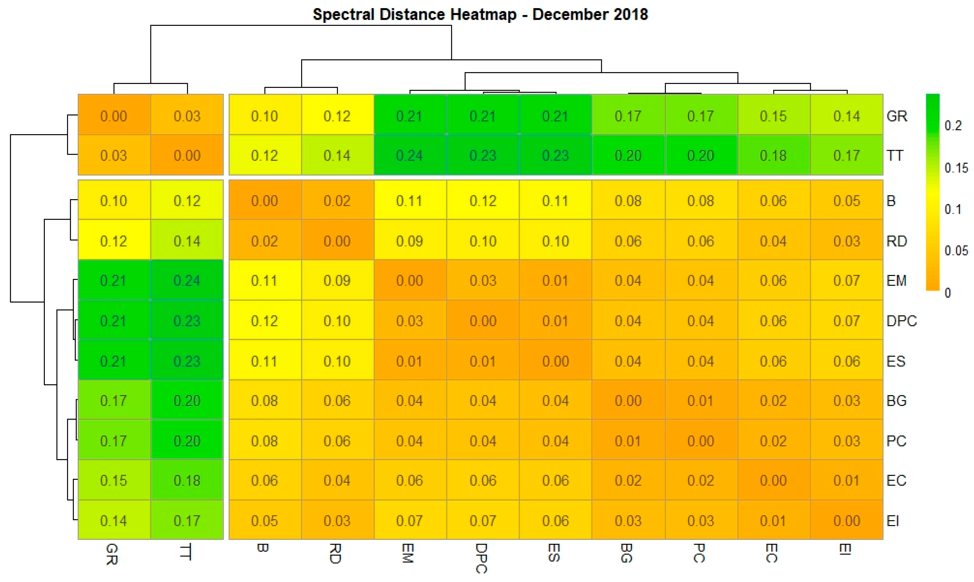
3.1. Differentiating Between Wetland Species Based on Their Spectral Signatures

This section presents the spectral distances and boxplots derived from the two dates. The larger distances represent higher spectral separation (Figure 7), highlighting the potential for spectral separation of plant species.
The results show that T. thermalis, E. mucronata, and R. dispar were the most distinguishable species. In contrast, the spectral differences between B. lanuginosa, B. gladiata, and G. rosmarinifolia were minimal, indicating potential challenges in accurately classifying these species in late spring. However, all three exhibited relatively higher spectral differences when compared to the Ericaceae family.
The corresponding box plots (Figure 8) revealed that T. thermalis, E. mucronata, and R. dispar had distinct reflectance patterns in the near-infrared, red edge, and red bands. Meanwhile, B. lanuginosa, B. gladiata, and G. rosmarinifolia displayed similar reflectance patterns, though indices utilizing the green and red bands might help amplify spectral differences between these species.
Notably, the spectral separability of B. lanuginosa and G. rosmarinifolia improved significantly in December 2018 (Figure 9). G. rosmarinifolia and T. thermalis emerged as the most spectrally distinct species relative to other species, but they were spectrally similar to each other. This improved separability may be attributed to pronounced reflectance differences in the red and near-infrared bands. However, the spectral distances in December 2018 were lower than those in October 2018, suggesting that late spring may be more favourable for spectral discrimination than summer. The results also demonstrate the impact of seasonality on species discrimination.
The corresponding box plots (Figure 10) revealed that G. rosmarinifolia, T. thermalis, and B. lanuginosa had distinct reflectance patterns in the green and red edge bands, suggesting that indices based on those bands might help amplify spectral differences between these species.

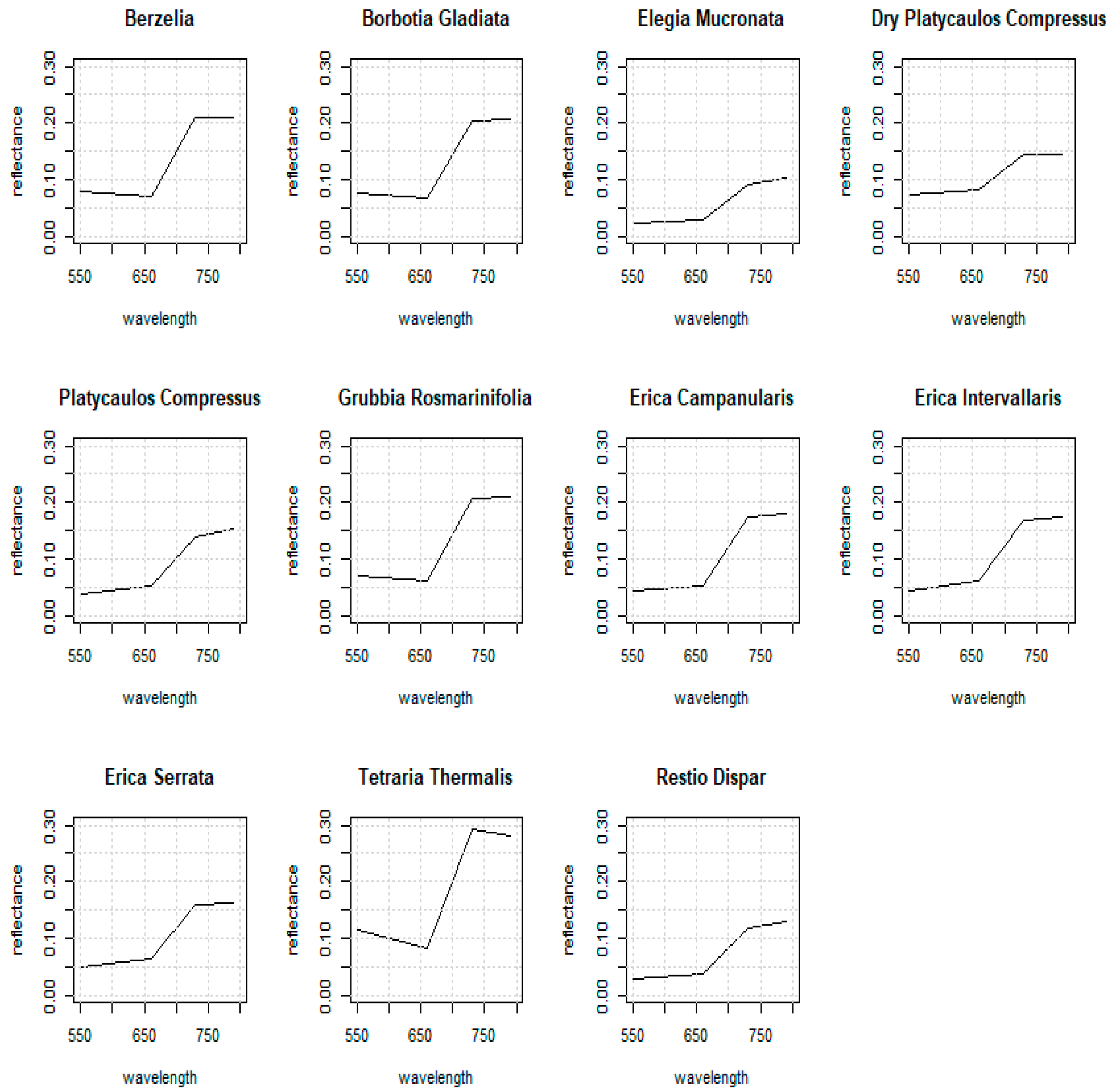
3.2. Inter-Seasonal Foliar Spectral Variations in the Species

This section presents the spectral reflectance curves derived from the two dates.

3.2.1. Berzelia lanuginosa

In October 2018, B. lanuginosa demonstrated the highest reflectance in the green and red bands (Figure 11). This consistently high reflectance suggests relatively high chlorophyll content, particularly during early spring. Additionally, this species exhibited a steep gradient between the red and NIR bands, further confirming its higher chlorophyll levels compared to other species. In December 2018, which corresponds to the summer months, the chlorophyll content remained elevated, as evidenced by its comparatively higher canopy reflectance in the NIR and red edge bands (Figure 12).

3.2.2. Borbotia gladiata

B. gladiata, like B. lanuginosa, showed the highest reflectance in the green and red bands during October 2018 (Figure 11). This is indicative of a relatively high chlorophyll content during those months. The presence of chlorophyll was further confirmed by a steep gradient observed between the red and near-infrared (NIR) bands, which remained prominent in December 2018 (Figure 12).

3.2.3. Grubbia rosmarinifolia

G. rosmarinifolia, along with B. lanuginosa and B. gladiata, showed high reflectance in the green and red bands in October 2018. The steep gradient between the red and NIR bands in these months further confirmed its high chlorophyll levels (Figure 11). In December 2018, G. rosmarinifolia continued to show relatively high chlorophyll content, demonstrated by its higher reflectance in the red edge and NIR bands (Figure 12).

3.2.4. Tetraria thermalis

T. thermalis exhibited the highest reflectance in both the green and red bands during October 2018, similar to B. lanuginosa, B. gladiata, and G. rosmarinifolia. Unlike the other species, T. thermalis demonstrated the largest gradient between the green and red bands, indicating a high chlorophyll content (Figure 11). However, in December 2018, the reflectance in the green band for T. thermalis decreased, while the red band reflectance remained high. This change suggests the possibility of vegetation stress, seasonal senescence, or an increase in anthocyanin content [83,84].

3.2.5. Erica intervallaris

E. intervallaris showed the lowest green reflectance in October 2018, which could be indicative of lower chlorophyll content or increased anthocyanin presence (Figure 11). Studies have shown that Ericaceae shrubs exhibit increased anthocyanins and reduced foliar chlorophyll in spring [85]. This trend continued into December 2018, when E. intervallaris exhibited lower reflectance in the green band compared to the red band. These characteristics suggest a potential response to environmental stresses or higher anthocyanin content. In contrast, during the same months, E. intervallaris exhibited higher reflectance in the red band, signalling a reduced chlorophyll presence (Figure 12).

3.2.6. Erica serrata

In line with E. intervallaris, E. serrata showed low green and higher red band reflectance in October 2018, signalling lower canopy chlorophyll (Figure 11). The increased reflectance in the red band and the overall lower green band reflectance suggest potential vegetation stress or increased anthocyanin levels. These characteristics remained consistent in December 2018 (Figure 12).

3.2.7. Elegia mucronata

E. mucronata showed the least reflectance in the red band in October 2018 (Figure 11). Its green and red band reflectance was generally similar, indicating a relatively low chlorophyll content, and this pattern continued through December 2018 (Figure 12).

3.2.8. Platycaulos compressus

P. compressus also displayed very low reflectance in the green band in October 2018, similar to E. mucronata. Its reflectance in the red band was comparable to its green band reflectance, indicating low chlorophyll content (Figure 11). This trend continued into December 2018, when the species continued to show relatively low reflectance in both bands (Figure 12).

3.2.9. Restio dispar

R. dispar exhibited very low green reflectance, comparable to that of E. mucronata and P. compressus. The species demonstrated reduced reflectance in the red band, with a consistent reflectance pattern observed between the red and green bands in October 2018 (Figure 11). By December 2018, R. dispar showed a slight increase in reflectance, particularly in the near-infrared (NIR) band, which suggests a rise in chlorophyll content (Figure 12).

3.2.10. Erica campanularis (and Restio leptostachyus)

E. campanularis and R. leptostachyus displayed similar reflectance trends to the Restionaceae plants, R. dispari, and E. mucronata, with relatively low reflectance in the green band and higher reflectance in the red band. The similarity in reflectance was likely influenced by the spectral reflectance of the R. leptostachyus, a Restionaceae, that coexisted with the Erica campanularis, an Ericaceae. In October 2018, this pattern indicated lower chlorophyll content or higher anthocyanin levels (Figure 11). These trends continued in December 2018, with increased reflectance in the NIR band indicating higher chlorophyll content (Figure 12).

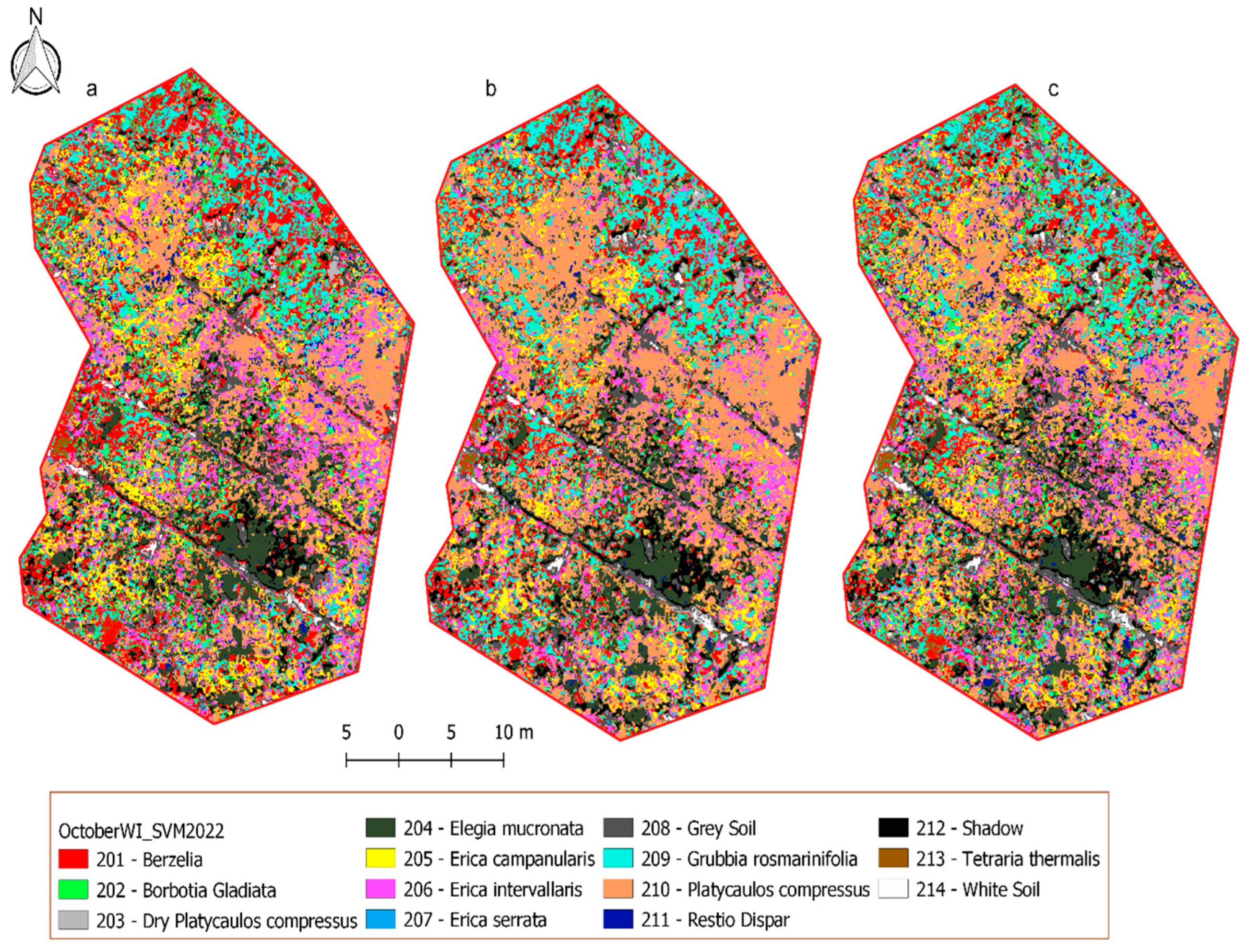
3.3. The Classification of the Wetland Species

Figure 13 and Figure 14 show the classification results for October 2018 and December 2018 respectively. The figures correspond to Support Vector Machines (SVMs), Random Forest (RF), and K Nearest Neighbour (KNN).
User accuracy is a metric for assessing the reliability of the classification to the user [86]. It is a measure of the pixels that are correctly classified against the total number of pixels in a class as per the classification [87]. It is the complementary metric of the commission error [88]. The producer accuracy reflects the extent to which the training pixels were correctly classified [89]. It is the complement of the omission error [88]. Random Forest had the best overall classification results, but the user and producer accuracies varied across the species (Table 4). The Supplementary Files contain the confusion matrices.
T. thermalis and E. mucronata had high user accuracies as anticipated from the spectral distances, but R. dispar was relatively poorly classified. This could be attributed to the limited classification data, as there were only three tufts in the wetland area. B. lanuginosa and E. serrata were also poorly classified with high commission errors. This is because of the spectral similarity to G. rosmarinifolia and Erica intervallaris, respectively (See Figure 9).
B. lanuginosa and E. serrata were also poorly classified in December 2018 (Table 5). The user accuracies of several species improved, with E. serrata, R. dispar, and T. thermalis showing the most significant gains. In contrast, the producer accuracies of B. lanuginosa, B. gladiata, and G. rosmarinifolia declined, indicating that more instances of these species were either omitted or incorrectly classified as other species. It is also evident that B. lanuginosa was overestimated in comparison to October 2018. The poor user accuracy is indicative of commission errors, particularly at the Southern boundary of the wetland (Figure 14). Notably, the KNN classifier performed better than RF and SVM at mapping the B. lanuginosa. This may indicate that the B. lanuginosa is irregularly distributed, but KNN can adapt since it makes decisions based on local neighbours.
These results contradict the spectral distance analysis, which showed a significant improvement in the spectral separability of B. lanuginosa and G. rosmarinifolia (Figure 10). A possible explanation is that B. lanuginosa had very limited coverage in the wetland, resulting in a small sample size, while G. rosmarinifolia was spectrally similar to T. thermalis, leading to classification challenges.

4. Conclusions

This study clearly met its main aim. First, it sought to explore the ability of UAV multispectral data to differentiate between wetland species based on their spectral signatures. Second, it examined the sensitivity of UAV multispectral data to inter-seasonal foliar spectral variations across different fynbos wetland species. Finally, it investigated the correlation between spectral differences among species and their classification accuracy using machine learning algorithms.
The relative spectral distances varied across species and seasons. UAV data successfully highlighted differences in reflectance across spectral bands for the two dates. Based on the spectral curves and box plots, it was evident that certain species were more likely to be classified accurately in October 2018 than in December 2018, and vice versa. These findings underscore the efficacy of UAV multispectral data in analyzing the reflectance patterns of fynbos wetland species. Furthermore, the sensitivity of multispectral sensors to foliar pigment composition across different seasonal stages was confirmed.
Euclidean spectral distances calculated from the reflectance data revealed distinct spectral clustering of plant species, which varied across different temporal intervals and included species from diverse plant families. These clusters highlighted which species could be discriminated from one another at specific dates and seasons. In October 2018, T. thermalis, E. mucronata, and R. dispar were the most distinguishable species. In December 2018, G. rosmarinifolia and T. thermalis emerged as the most spectrally distinct species relative to others, though they were spectrally similar to each other.
Lastly, species classification results demonstrated that a random forest classifier is well suited for this task. The relative producer and user accuracies aligned with the spectral distance calculations and box plots. While most species were classified accurately, B. lanuginosa, E. serrata, and R. dispar warrant further investigation. Conservation efforts in the CFR must be backed by updated information about the local vegetation. The methods demonstrated in this study provide a means for municipal officials to remotely monitor seep wetlands and the changes at the species level. Future research should assess the influence of spectral indices and seasonality on these species and should explore the use of high-resolution satellite data with similar or higher spectral resolutions. Additionally, more data should be collected across all seasons to determine the optimal time of year for optimum plant species discrimination.

Supplementary Materials

The following supporting information can be downloaded at: https://www.mdpi.com/article/10.3390/geomatics5020017/s1.

Author Contributions

Conceptualization, K.M.; methodology, K.M., M.S., and J.S.; software, K.M.; validation, K.M.; formal analysis, K.M.; investigation, K.M.; resources, K.M., M.S., and J.S.; data curation, K.M.; writing—original draft preparation, K.M.; writing—review and editing, K.M., M.S., and J.S.; visualization, K.M.; supervision, M.S. and J.S.; project administration, M.S. and J.S. All authors have read and agreed to the published version of the manuscript.

Funding

This research received no external funding.

Institutional Review Board Statement

Not applicable.

Informed Consent Statement

Not applicable.

Data Availability Statement

The datasets presented in this article are not readily available because the data are part of an ongoing study. Requests to access the datasets should be directed to the corresponding author.

Acknowledgments

We are thankful to the botanists who assisted with identifying the plant species in the field. We are also grateful to theUCT Biological Sciences Department and Drone Solutions International for assistance with capturing the drone data used in this study.

Conflicts of Interest

The authors declare no conflicts of interest.

References

  1. Turpie, J.K.; Heydenrych, B.J.; Lamberth, S.J. Economic Value of Terrestrial and Marine Biodiversity in the Cape Floristic Region: Implications for Defining Effective and Socially Optimal Conservation Strategies. Biol. Conserv. 2003, 112, 233–251. [Google Scholar] [CrossRef]
  2. Bek, D.; O’grady, K. The Scale, Structure and Sustainability of the Wild Fynbos Harvesting Supply Chain in the Cape Floral Kingdom; Coventry University: Coventry, UK, 2018. [Google Scholar]
  3. Bossi, L. Mapping Cape Fynbos Vegetation with the Aid of Landsat Imagery. Veld Flora 1984, 70, 31–33. [Google Scholar]
  4. Helme, N.A.; Trinder-Smith, T.H. The Endemic Flora of the Cape Peninsula, South Africa. S. Afr. J. Bot. 2006, 72, 205–210. [Google Scholar] [CrossRef]
  5. Rebelo, A.G.; Boucher, C.; Helme, N. Fynbos Biome. In The Vegetation of South Africa, Lesotho and Swaziland; Mucina, L., Rutherford, M.C., Eds.; SANBI: Pretoria, South Africa, 2006; pp. 53–219. [Google Scholar]
  6. Wittridge, H.-M. Integrated Reserve Management Plan—Steenbras Nature Reserve; City of Cape Town: Cape Town, South Africa, 2011. [Google Scholar]
  7. Ewart-Smith, J.; Boucher, C. Baseline Assessment of Ecosystems Potentially Impacted by The Well-Field Development at Steenbras; Freshwater Consulting Group: Cape Town, South Africa, 2019. [Google Scholar]
  8. West, S.; Cairns, R.; Schultz, L. What Constitutes a Successful Biodiversity Corridor? A Q-Study in the Cape Floristic Region, South Africa. Biol. Conserv. 2016, 198, 183–192. [Google Scholar] [CrossRef]
  9. Topp, E.N.; Loos, J.; Martín-López, B. Decision-Making for Nature’s Contributions to People in the Cape Floristic Region: The Role of Values, Rules and Knowledge. Sustain. Sci. 2022, 17, 739–760. [Google Scholar] [CrossRef]
  10. Van Wilgen, B.W. The Evolution of Fire and Invasive Alien Plant Management Practices in Fynbos. S. Afr. J. Sci. 2009, 105, 335–342. [Google Scholar] [CrossRef]
  11. van Wilgen, B. Plantation Forestry and Invasive Pines in the Cape Floristic Region: Towards Conflict Resolution. S. Afr. J. Sci. 2015, 111, 1–2. [Google Scholar] [CrossRef]
  12. Kraaij, T.; Baard, J.A.; Rikhotso, D.R.; Cole, N.S.; Van Wilgen, B.W. Assessing the Effectiveness of Invasive Alien Plant Management in a Large Fynbos Protected Area. Bothalia 2017, 47, a2105. [Google Scholar] [CrossRef]
  13. Rebelo, A.G.; Holmes, P.M.; Dorse, C.; Wood, J. Impacts of Urbanization in a Biodiversity Hotspot: Conservation Challenges in Metropolitan Cape Town. S. Afr. J. Bot. 2011, 77, 20–35. [Google Scholar] [CrossRef]
  14. Kingsford, R.T.; Basset, A.; Jackson, L. Wetlands: Conservation’s Poor Cousins. Aquat. Conserv. 2016, 26, 892–916. [Google Scholar] [CrossRef]
  15. Sieben, E.J.J.; Glen, R.P.; van Deventer, H.; Dayaram, A. The Contribution of Wetland Flora to Regional Floristic Diversity across a Wide Range of Climatic Conditions in Southern Africa. Biodivers. Conserv. 2021, 30, 575–596. [Google Scholar] [CrossRef]
  16. Adam, E.; Mutanga, O. Spectral Discrimination of Papyrus Vegetation (Cyperus Papyrus L.) in Swamp Wetlands Using Field Spectrometry. ISPRS J. Photogramm. Remote Sens. 2009, 64, 612–620. [Google Scholar] [CrossRef]
  17. Gallant, A. The Challenges of Remote Monitoring of Wetlands. Remote Sens. 2015, 7, 10938–10950. [Google Scholar] [CrossRef]
  18. Harris, B.L.; Taylor, C.M.; Weedon, G.P.; Talib, J.; Dorigo, W.; van der Schalie, R. Satellite-Observed Vegetation Responses to Intraseasonal Precipitation Variability. Geophys. Res. Lett. 2022, 49, e2022GL099635. [Google Scholar] [CrossRef]
  19. Mishra, D.R.; Ghosh, S.; Hladik, C.; O’Connell, J.L.; Cho, H.J. Wetland Mapping Methods and Techniques Using Multisensor, Multiresolution Remote Sensing: Successes and Challenges. In Remote Sensing Handbook; Thenkabail, P.S., Ed.; Taylor and Francis: New York, NY, USA, 2015; Volume 3, pp. 191–226. ISBN 0780312406. [Google Scholar]
  20. Ozer, E.; Leloglu, U.M. Wetland Spectral Unmixing Using Multispectral Satellite Images. Geocarto Int. 2022, 37, 15754–15777. [Google Scholar] [CrossRef]
  21. Jiang, J.; Johansen, K.; Tu, Y.-H.; McCabe, M.F. Multi-Sensor and Multi-Platform Consistency and Interoperability between UAV, Planet CubeSat, Sentinel-2, and Landsat Reflectance Data. GIsci Remote Sens. 2022, 59, 936–958. [Google Scholar] [CrossRef]
  22. Fu, B.; Li, S.; Lao, Z.; Yuan, B.; Liang, Y.; He, W.; Sun, W.; He, H. Multi-Sensor and Multi-Platform Retrieval of Water Chlorophyll a Concentration in Karst Wetlands Using Transfer Learning Frameworks with ASD, UAV, and Planet CubeSate Reflectance Data. Sci. Total Environ. 2023, 901, 165963. [Google Scholar] [CrossRef]
  23. Islam, M.K.; Simic Milas, A.; Abeysinghe, T.; Tian, Q. Integrating UAV-Derived Information and WorldView-3 Imagery for Mapping Wetland Plants in the Old Woman Creek Estuary, USA. Remote Sens. 2023, 15, 1090. [Google Scholar] [CrossRef]
  24. Park, S.-I.; Hwang, Y.-S.; Lee, J.-J.; Um, J.-S. Evaluating Operational Potential of UAV Transect Mapping for Wetland Vegetation Survey. J. Coast. Res. 2021, 114. [Google Scholar] [CrossRef]
  25. Van Alphen, R.; Rains, K.C.; Rodgers, M.; Malservisi, R.; Dixon, T.H. UAV-Based Wetland Monitoring: Multispectral and Lidar Fusion with Random Forest Classification. Drones 2024, 8, 113. [Google Scholar] [CrossRef]
  26. Wang, C.; Pavelsky, T.M.; Kyzivat, E.D.; Garcia-Tigreros, F.; Podest, E.; Yao, F.; Yang, X.; Zhang, S.; Song, C.; Langhorst, T.; et al. Quantification of Wetland Vegetation Communities Features with Airborne AVIRIS-NG, UAVSAR, and UAV LiDAR Data in Peace-Athabasca Delta. Remote Sens. Environ. 2023, 294, 113646. [Google Scholar] [CrossRef]
  27. Ramjukadh, C.-L. Are Wetland Plant Communities in the Cape Flora Influenced by Environmental and Land-Use Changes? Master’s Thesis, University of Cape Town, Cape Town, South Africa, 2014. [Google Scholar]
  28. Duncan, P.; Lewarne, M. Using Remote Sensing and GIS Techniques to Detect Changes to the Prince Alfred Hamlet Conservation Area in the Western Cape, South Africa. ISPRS—Int. Arch. Photogramm. Remote Sens. Spat. Inf. Sci. 2016, XLI-B7, 475–481. [Google Scholar] [CrossRef]
  29. Thamaga, K.H.; Dube, T.; Shoko, C. Evaluating the Impact of Land Use and Land Cover Change on Unprotected Wetland Ecosystems in the Arid-Tropical Areas of South Africa Using the Landsat Dataset and Support Vector Machine. Geocarto Int. 2022, 37, 10344–10365. [Google Scholar] [CrossRef]
  30. Hope, A.; Albers, N.; Bart, R. Characterizing Post-Fire Recovery of Fynbos Vegetation in the Western Cape Region of South Africa Using MODIS Data. Int. J. Remote Sens. 2012, 33, 979–999. [Google Scholar] [CrossRef]
  31. Wilson, A.M.; Latimer, A.M.; Silander, J.A. Climatic Controls on Ecosystem Resilience: Postfire Regeneration in the Cape Floristic Region of South Africa. Proc. Natl. Acad. Sci. USA 2015, 112, 9058–9063. [Google Scholar] [CrossRef] [PubMed]
  32. van Blerk, J.J.; West, A.G.; Smit, J.; Altwegg, R.; Hoffman, M.T. UAVs Improve Detection of Seasonal Growth Responses during Post-Fire Shrubland Recovery. Landsc. Ecol. 2022, 37, 3179–3199. [Google Scholar] [CrossRef]
  33. Beckett, H. Remote-Sensing of Water Stress in Fynbos Vegetation. Honours Thesis, University of Cape Town, Cape Town, South Africa, 2010. [Google Scholar]
  34. Jovanovic, N.; Garcia, C.L.; Bugan, R.D.H.; Teich, I.; Rodriguez, C.M.G. Validation of Remotely-Sensed Evapotranspiration and NDWI Using Ground Measurements at Riverlands, South Africa. Water SA 2014, 40, 211–220. [Google Scholar] [CrossRef]
  35. Skowno, A.L.; Jewitt, D.; Slingsby, J.A. Rates and Patterns of Habitat Loss across South Africa’s Vegetation Biomes. S. Afr. J. Sci. 2021, 117, 1–6. [Google Scholar] [CrossRef]
  36. Mtengwana, B.; Dube, T.; Mudereri, B.T.; Shoko, C. Modeling the Geographic Spread and Proliferation of Invasive Alien Plants (IAPs) into New Ecosystems Using Multi-Source Data and Multiple Predictive Models in the Heuningnes Catchment, South Africa. GIsci Remote Sens. 2021, 58, 483–500. [Google Scholar] [CrossRef]
  37. Mtengwana, B.; Dube, T.; Mkunyana, Y.P.; Mazvimavi, D. Use of Multispectral Satellite Datasets to Improve Ecological Understanding of the Distribution of Invasive Alien Plants in a Water-Limited Catchment, South Africa. Afr. J. Ecol. 2020, 58, 709–718. [Google Scholar] [CrossRef]
  38. Shoko, C.; Mutanga, O.; Dube, T. Remotely Sensed Characterization of Acacia Longifolia Invasive Plants in the Cape Floristic Region of the Western Cape, South Africa. J. Appl. Remote Sens. 2020, 14, 044511. [Google Scholar] [CrossRef]
  39. Duncan, P.; Podest, E.; Esler, K.J.; Geerts, S.; Lyons, C. Mapping Invasive Herbaceous Plant Species with Sentinel-2 Satellite Imagery: Echium Plantagineum in a Mediterranean Shrubland as a Case Study. Geomatics 2023, 3, 328–344. [Google Scholar] [CrossRef]
  40. Seymour, D. Wetland Ecotones: Testing Remote Sensing Techniques to Map Ecotones in A Fynbos Embedded Wetland; Stellenbosch University: Stellenbosch, South Africa, 2022. [Google Scholar]
  41. van Blerk, J.J.; Cramer, M.D.; West, A.G.; Musker, S.D.; Verboom, G.A. The Contribution of Hydric Habitats to the Richness of the Cape Fynbos Flora. Divers. Distrib. 2025, 31, e13962. [Google Scholar] [CrossRef]
  42. Ndebele, N.E.; Grab, S.; Hove, H. Wet Season Rainfall Characteristics and Temporal Changes for Cape Town, South Africa, 1841–2018. Clim. Past. 2022, 18, 2463–2482. [Google Scholar] [CrossRef]
  43. Roffe, S.J.; Steinkopf, J.; Fitchett, J.M. South African Winter Rainfall Zone Shifts: A Comparison of Seasonality Metrics for Cape Town from 1841–1899 and 1933–2020. Theor. Appl. Climatol. 2022, 147, 1229–1247. [Google Scholar] [CrossRef]
  44. Martínez-Carricondo, P.; Agüera-Vega, F.; Carvajal-Ramírez, F.; Mesas-Carrascosa, F.J.; García-Ferrer, A.; Pérez-Porras, F.J. Assessment of UAV-Photogrammetric Mapping Accuracy Based on Variation of Ground Control Points. Int. J. Appl. Earth Obs. Geoinf. 2018, 72, 1–10. [Google Scholar] [CrossRef]
  45. Ntuli, S.; Forbes, A. Classification of 3D UAS-SfM Point Clouds in the Urban Environment. S. Afr. J. Geomat. 2023, 12, 190–205. [Google Scholar] [CrossRef]
  46. Onwudinjo, K.C.; Smit, J. Estimating the Performance of Multi-Rotor Unmanned Aerial Vehicle Structure-from-Motion (UAVsfm) Imagery in Assessing Homogeneous and Heterogeneous Forest Structures: A Comparison to Airborne and Terrestrial Laser Scanning. S. Afr. J. Geomat. 2022, 11, 65–83. [Google Scholar] [CrossRef]
  47. Zeng, C.; Richardson, M.; King, D.J. The Impacts of Environmental Variables on Water Reflectance Measured Using a Lightweight Unmanned Aerial Vehicle (UAV)-Based Spectrometer System. ISPRS J. Photogramm. Remote Sens. 2017, 130, 217–230. [Google Scholar] [CrossRef]
  48. Tmušić, G.; Manfreda, S.; Aasen, H.; James, M.R.; Gonçalves, G.; Ben-Dor, E.; Brook, A.; Polinova, M.; Arranz, J.J.; Mészáros, J.; et al. Current Practices in UAS-Based Environmental Monitoring. Remote Sens. 2020, 12, 1001. [Google Scholar] [CrossRef]
  49. Delavarpour, N.; Koparan, C.; Nowatzki, J.; Bajwa, S.; Sun, X. A Technical Study on UAV Characteristics for Precision Agriculture Applications and Associated Practical Challenges. Remote Sens. 2021, 13, 1204. [Google Scholar] [CrossRef]
  50. Cramer, M.; Przybilla, H.-J.; Zurhorst, A. UAV Cameras: Overview and Geometric Calibration Benchmark. Int. Arch. Photogramm. Remote Sens. Spat. Inf. Sci. 2017, XLII-2/W6, 85–92. [Google Scholar] [CrossRef]
  51. Przybilla, H.-J.; Bäumker, M.; Luhmann, T.; Hastedt, H.; Eilers, M. Interaction Between Direct Georeferencing, Control Point Configuration and Camera Self-Calibration for RTK-Based UAV Photogrammetry. Int. Arch. Photogramm. Remote Sens. Spat. Inf. Sci. 2020, XLIII-B1-2020, 485–492. [Google Scholar] [CrossRef]
  52. Sai, S.S.; Tjahjadi, M.E.; Rokhmana, C.A. Geometric Accuracy Assessments of Orthophoto Production From UAV Aerial Images. In Proceedings of the 1st International Conference on Geodesy, Geomatics, and Land Administration 2019, Semarang, Indonesia, 24–25 July 2019; KnE Engineering: Semarang, Indonesia, 2019; pp. 333–344. [Google Scholar] [CrossRef]
  53. Nex, F.; Remondino, F. UAV for 3D Mapping Applications: A Review. Appl. Geomat. 2014, 6, 1–15. [Google Scholar] [CrossRef]
  54. Zhou, Y.; Rupnik, E.; Meynard, C.; Thom, C.; Pierrot-Deseilligny, M. Simulation and Analysis of Photogrammetric UAV Image Blocks—Influence of Camera Calibration Error. Remote Sens. 2019, 12, 22. [Google Scholar] [CrossRef]
  55. Harwin, S.; Lucieer, A.; Osborn, J. The Impact of the Calibration Method on the Accuracy of Point Clouds Derived Using Unmanned Aerial Vehicle Multi-View Stereopsis. Remote Sens. 2015, 7, 11933–11953. [Google Scholar] [CrossRef]
  56. Mathews, A. A Practical UAV Remote Sensing Methodology to Generate Multispectral Orthophotos for Vineyards: Estimation of Spectral Reflectance. Int. J. Appl. Geospat. Res. 2015, 6, 65–87. [Google Scholar] [CrossRef]
  57. Cao, S.; Danielson, B.; Clare, S.; Koenig, S.; Campos-Vargas, C.; Sanchez-Azofeifa, A. Radiometric Calibration Assessments for UAS-Borne Multispectral Cameras: Laboratory and Field Protocols. ISPRS J. Photogramm. Remote Sens. 2019, 149, 132–145. [Google Scholar] [CrossRef]
  58. Daniels, L.; Eeckhout, E.; Wieme, J.; Dejaegher, Y.; Audenaert, K.; Maes, W.H. Identifying the Optimal Radiometric Calibration Method for UAV-Based Multispectral Imaging. Remote Sens. 2023, 15, 2909. [Google Scholar] [CrossRef]
  59. Cubero-Castan, M.; Schneider-Zapp, K.; Bellomo, M.; Shi, D.; Rehak, M.; Strecha, C. Assessment of The Radiometric Accuracy in A Target Less Work Flow Using Pix4D Software. In Proceedings of the 2018 9th Workshop on Hyperspectral Image and Signal Processing: Evolution in Remote Sensing (WHISPERS), Amsterdam, The Netherlands, 23–26 September 2018; IEEE: New York, NY, USA, 2018; pp. 1–4. [Google Scholar]
  60. Schneider-Zapp, K.; Cubero-Castan, M.; Shi, D.; Strecha, C. A New Method to Determine Multi-Angular Reflectance Factor from Lightweight Multispectral Cameras with Sky Sensor in a Target-Less Workflow Applicable to UAV. Remote Sens. Environ. 2019, 229, 60–68. [Google Scholar] [CrossRef]
  61. Zhu, H.; Huang, Y.; An, Z.; Zhang, H.; Han, Y.; Zhao, Z.; Li, F.; Zhang, C.; Hou, C. Assessing Radiometric Calibration Methods for Multispectral UAV Imagery and the Influence of Illumination, Flight Altitude and Flight Time on Reflectance, Vegetation Index and Inversion of Winter Wheat AGB and LAI. Comput. Electron. Agric. 2024, 219, 108821. [Google Scholar] [CrossRef]
  62. Avtar, R.; Suab, S.A.; Syukur, M.S.; Korom, A.; Umarhadi, D.A.; Yunus, A.P. Assessing the Influence of UAV Altitude on Extracted Biophysical Parameters of Young Oil Palm. Remote Sens. 2020, 12, 3030. [Google Scholar] [CrossRef]
  63. Guo, Y.; Senthilnath, J.; Wu, W.; Zhang, X.; Zeng, Z.; Huang, H. Radiometric Calibration for Multispectral Camera of Different Imaging Conditions Mounted on a UAV Platform. Sustainability 2019, 11, 978. [Google Scholar] [CrossRef]
  64. Shetty, S.; Gupta, P.K.; Belgiu, M.; Srivastav, S.K. Assessing the Effect of Training Sampling Design on the Performance of Machine Learning Classifiers for Land Cover Mapping Using Multi-Temporal Remote Sensing Data and Google Earth Engine. Remote Sens. 2021, 13, 1433. [Google Scholar] [CrossRef]
  65. Dimov, D. Classification of Remote Sensing Time Series and Similarity Metrics for Crop Type Verification. J. Appl. Remote Sens. 2022, 16, 024519. [Google Scholar] [CrossRef]
  66. Li, X.; Li, J.; Jiang, J.; Pan, X.; Huang, X. Spatio-Temporal-Text Fusion for Hierarchical Multi-Label Crop Classification Based on Time-Series Remote Sensing Imagery. Int. J. Appl. Earth Obs. Geoinf. 2025, 139, 104471. [Google Scholar] [CrossRef]
  67. Deng, J.; Dong, W.; Guo, Y.; Chen, X.; Zhou, R.; Liu, W. A Novel Remote Sensing Image Enhancement Method, the Pseudo-Tasseled Cap Transformation: Taking Buildings and Roads in GF-2 as an Example. Appl. Sci. 2023, 13, 6585. [Google Scholar] [CrossRef]
  68. Yu, L.; Luo, X.; Croft, H.; Rogers, C.A.; Chen, J.M. Seasonal Variation in the Relationship between Leaf Chlorophyll Content and Photosynthetic Capacity. Plant Cell Environ. 2024, 47, 3953–3965. [Google Scholar] [CrossRef]
  69. Connelly, L.M. Introduction to Analysis of Variance (ANOVA). MEDSURG Nurs. 2021, 30, 218. [Google Scholar] [CrossRef]
  70. Fraser, D.A.S. The P-Value Function and Statistical Inference. Am. Stat. 2019, 73, 135–147. [Google Scholar] [CrossRef]
  71. Guo, M.; Li, J.; Sheng, C.; Xu, J.; Wu, L. A Review of Wetland Remote Sensing. Sensors 2017, 17, 777. [Google Scholar] [CrossRef] [PubMed]
  72. Mahdianpari, M.; Granger, J.E.; Mohammadimanesh, F.; Salehi, B.; Brisco, B.; Homayouni, S.; Gill, E.; Huberty, B.; Lang, M. Meta-Analysis of Wetland Classification Using Remote Sensing: A Systematic Review of a 40-Year Trend in North America. Remote Sens. 2020, 12, 1882. [Google Scholar] [CrossRef]
  73. Mahdavi, S.; Salehi, B.; Granger, J.; Amani, M.; Brisco, B.; Huang, W. Remote Sensing for Wetland Classification: A Comprehensive Review. GIsci Remote Sens. 2018, 55, 623–658. [Google Scholar] [CrossRef]
  74. Thanh Noi, P.; Kappas, M. Comparison of Random Forest, k-Nearest Neighbor, and Support Vector Machine Classifiers for Land Cover Classification Using Sentinel-2 Imagery. Sensors 2017, 18, 18. [Google Scholar] [CrossRef]
  75. Judah, A.; Hu, B. The Integration of Multi-Source Remotely-Sensed Data in Support of the Classification of Wetlands. Remote Sens. 2019, 11, 1537. [Google Scholar] [CrossRef]
  76. Farda, N.M. Multi-Temporal Land Use Mapping of Coastal Wetlands Area Using Machine Learning in Google Earth Engine. IOP Conf. Ser. Earth Environ. Sci. 2017, 98, 012042. [Google Scholar] [CrossRef]
  77. Okolie, C.; Adeleke, A.; Mills, J.; Smit, J.; Maduako, I.; Bagheri, H.; Komar, T.; Wang, S. Assessment of Explainable Tree-Based Ensemble Algorithms for the Enhancement of Copernicus Digital Elevation Model in Agricultural Lands. Int. J. Image Data Fusion. 2024, 15, 430–460. [Google Scholar] [CrossRef]
  78. Raczko, E.; Zagajewski, B. Comparison of Support Vector Machine, Random Forest and Neural Network Classifiers for Tree Species Classification on Airborne Hyperspectral APEX Images. Eur. J. Remote Sens. 2017, 50, 144–154. [Google Scholar] [CrossRef]
  79. Boateng, E.Y.; Otoo, J.; Abaye, D.A. Basic Tenets of Classification Algorithms K-Nearest-Neighbor, Support Vector Machine, Random Forest and Neural Network: A Review. J. Data Anal. Inf. Process. 2020, 8, 341–357. [Google Scholar] [CrossRef]
  80. Rummell, A.J.; Leon, J.X.; Borland, H.P.; Elliott, B.B.; Gilby, B.L.; Henderson, C.J.; Olds, A.D. Watching the Saltmarsh Grow: A High-Resolution Remote Sensing Approach to Quantify the Effects of Wetland Restoration. Remote Sens. 2022, 14, 4559. [Google Scholar] [CrossRef]
  81. Fallah, M.; Reza, A.; Zefrehei, P.; Aliakbar Hedayati, S.; Bagheri, T. Comparison of Temporal and Spatial Patterns of Water Quality Parameters in Anzali Wetland (Southwest of the Caspian Sea) Using Support Vector Machine Model. Casp. J. Environ. Sci. 2021, 19, 95–104. [Google Scholar] [CrossRef]
  82. Magidi, J.; Bangira, T.; Kelepile, M.; Shoko, M. Land Use and Land Cover Changes in Notwane Watershed, Bot-swana, Using Extreme Gradient Boost (XGBoost) Machine Learning Algorithm. Afr. Geogr. Rev. 2024, 1–21. [Google Scholar] [CrossRef]
  83. Steele, M.R.; Gitelson, A.A.; Rundquist, D.C.; Merzlyak, M.N. Nondestructive Estimation of Anthocyanin Content in Grapevine Leaves. Am. J. Enol. Vitic. 2009, 60, 87–92. [Google Scholar] [CrossRef]
  84. Viña, A.; Gitelson, A.A. Sensitivity to Foliar Anthocyanin Content of Vegetation Indices Using Green Reflectance. IEEE Geosci. Remote Sens. Lett. 2011, 8, 464–468. [Google Scholar] [CrossRef]
  85. Bayle, A.; Carlson, B.; Thierion, V.; Isenmann, M.; Choler, P. Improved Mapping of Mountain Shrublands Using the Sentinel-2 Red-Edge Band. Remote Sens. 2019, 11, 2807. [Google Scholar] [CrossRef]
  86. Rwanga, S.S.; Ndambuki, J.M. Accuracy Assessment of Land Use/Land Cover Classification Using Remote Sensing and GIS. Int. J. Geosci. 2017, 8, 611–622. [Google Scholar] [CrossRef]
  87. Story, M.; Congalton, R.G. Remote Sensing Brief Accuracy Assessment: A User’s Perspective. Photogramm. Eng. Remote Sens. 1986, 52, 397–399. [Google Scholar]
  88. Olofsson, P.; Foody, G.M.; Herold, M.; Stehman, S.V.; Woodcock, C.E.; Wulder, M.A. Good Practices for Estimating Area and Assessing Accuracy of Land Change. Remote Sens. Environ. 2014, 148, 42–57. [Google Scholar] [CrossRef]
  89. Barsi, Á.; Kugler, Z.; László, I.; Szabó, G.; Abdulmutalib, H.M. Accuracy Dimensions in Remote Sensing. Int. Arch. Photogramm. Remote Sens. Spat. Inf. Sci. 2018, XLII–3, 61–67. [Google Scholar] [CrossRef]
Figure 1. The study area (Google Earth imagery and UAV RGB composites).
Geomatics 05 00017 g001
Figure 2. The dominant plant species in the wetland. The plant species are as follows: (a). Tetraria thermalis; (b). Borbotia gladiata; (c). Restio dispar; (d). Berzelia lanuginosa; (e). Platycaulos compressus; (f). Grubbia rosmarinifolia; (g). Erica intervallaris; (h). Erica serrata; (i). Elegia mucronata; (j). Erica campanularis (with narrow-linear leaves) and Restio leptostachyus (with a grassy appearance); (k). Erica campanularis (with its yellow flowers) alongside Restio leptostachyus (with a grassy appearance) in the wetland.
Geomatics 05 00017 g002
Figure 3. Ground Control Points used during the study (Municipal Aerial RGB photo).
Geomatics 05 00017 g003
Figure 4. Application of reflectance factors on the green band calibration photos. The digitised rectangle denotes the area showing the reflectance in the green band. The value 0.72 is the reflectance factor.
Geomatics 05 00017 g004
Figure 5. Ground truth GNSS positions of the dominant plant species in the wetland.
Geomatics 05 00017 g005
Figure 6. Flowchart of the methodology used in this study.
Geomatics 05 00017 g006
Figure 7. Spectral distance results for October 2018. The class labels in the figure represent the key plant species as follows: B (Berzelia lanuginosa), BG (Borbotia gladiata), DPC (Dry or Dead Platycaulos Compressus), EM (Elegia mucronata), EC (Erica campanularis and Restio leptostachyus), EI (Erica intervallaris), ES (Erica serrata), GR (Grubbia rosmarinifolia), PC (Platycaulos compressus), RD (Restio dispar), and TT represents Tetraria thermalis.
Geomatics 05 00017 g007
Figure 8. Box plot of spectral distance results for October 2018. The class labels in the figure are as per the preceding figure. The figure plots are sorted by the median.
Geomatics 05 00017 g008
Figure 9. Spectral distance results for December 2018.
Geomatics 05 00017 g009
Figure 10. Box plot of spectral distance results for December 2018. The figure plots are sorted by the median.
Geomatics 05 00017 g010
Figure 11. Spectral curves from October 2018.
Geomatics 05 00017 g011
Figure 12. Spectral curves from December 2018.
Geomatics 05 00017 g012
Figure 13. Classification results for October 2018. (a) SVM. (b) Random Forest. (c) KNN.
Geomatics 05 00017 g013
Figure 14. Classification results for December 2018. (a) SVM. (b) Random Forest. (c) KNN.
Geomatics 05 00017 g014
Table 1. Dominant plant species.
Plant NamePlant FamilyAverage HeightLeaves
Berzelia lanuginosaBruniaceae1.5 mSmall and narrow in whorls
Bobartia gladiataIridaceae0.8 mRigid ensiform
Elegia mucronataRestionaceae2.0 mStout erect sheaths
Erica campanularisEricaceae0.7 mSmall needle-like
Erica intervallarisEricaceae0.7 mIncurved, erect squarrose
Erica serrataEricaceae0.7 mSerrated edges
Grubbia rosmarinifoliaGrubbiaceae1.3 mGlossy narrow lanceolate
Platycaulos compressusRestionaceae0.5 mLong and narrow
Restio disparRestionaceae1.0 mReed like tufts
Restio leptostachyusRestionaceae0.5 mFeathery plume-like spikelets
Tetraria thermalisCyperaceae0.4 mDrooping sword-shaped
Table 2. Flight details.
DateTimeSensorSeason
4 October 201810 h 45Parrot SequoiaLate Spring
10 December 201814 h 57Parrot SequoiaEarly Summer
Table 3. Spectral properties of the Parrot Sequoia.
BandsCentre Wavelength (nm)Bandwidth (nm)Reflectance Factor
Green550400.72
Red660400.73
Red Edge735100.72
Near-infrared790400.69
Table 4. Classification results for October 2018.
ClassesBBGDPCEMECEIESGRPCRDTT
RF—Overall Accuracy [%] = 87.4%      Kappa = 0.85
PA [%]85.183.888.094.788.389.735.474.893.047.387.2
UA [%]66.785.392.992.873.283.557.590.296.960.782.7
Kappa0.630.850.930.920.720.820.570.880.960.60.83
SVM—Overall Accuracy [%] = 83.6%      Kappa = 0.81
PA [%]89.785.378.596.087.984.542.167.685.846.596.3
UA [%]66.475.894.690.572.976.473.793.096.653.180.9
Kappa0.620.750.940.890.700.740.730.920.960.520.81
KNN—Overall Accuracy [%] = 85.5%      Kappa = 0.83
PA [%]85.889.077.993.690.188.953.174.686.465.976.2
UA [%]72.274.596.392.374.276.569.693.096.357.474.5
Kappa0.690.740.960.910.720.740.690.920.950.560.74
Table 5. Classification Results for December 2018.
ClassesBBGDPCEMECEIESGRPCRDTT
RF—Overall Accuracy [%] = 88.0%      Kappa = 0.86
PA [%]33.569.1100.0100.096.286.931.665.699.264.5100.0
UA [%]13.275.0100.092.575.084.0100.095.795.0100.0100.0
Kappa0.110.741.000.920.730.831.000.950.941.001.00
SVM—Overall Accuracy [%] = 61.9%      Kappa = 0.56
PA [%]95.637.421.1100.073.246.833.764.892.23.26.1
UA [%]33.822.2100.090.280.073.985.796.093.0100.0100.0
Kappa0.210.191.000.900.780.700.860.950.921.001.00
KNN—Overall Accuracy [%] = 85.7%      Kappa = 0.83
PA [%]69.818.7100.0100.092.379.854.877.293.922.0100.0
UA [%]53.812.5100.075.581.368.660.096.990.9100.0100.0
Kappa0.510.091.000.740.800.670.590.970.891.001.00
Disclaimer/Publisher’s Note: The statements, opinions and data contained in all publications are solely those of the individual author(s) and contributor(s) and not of MDPI and/or the editor(s). MDPI and/or the editor(s) disclaim responsibility for any injury to people or property resulting from any ideas, methods, instructions or products referred to in the content.

