Article

Conditional Feature Selection: Evaluating Model Averaging When Selecting Features with Shapley Values

Department of Computer Science IV, University of Bonn, 53121 Bonn, Germany
*
Authors to whom correspondence should be addressed.
Geomatics 2024, 4(3), 286-310; https://doi.org/10.3390/geomatics4030016
Submission received: 3 July 2024 / Revised: 25 July 2024 / Accepted: 6 August 2024 / Published: 8 August 2024

Abstract

:
In the field of geomatics, artificial intelligence (AI) and especially machine learning (ML) are rapidly transforming the field of geomatics with respect to collecting, managing, and analyzing spatial data. Feature selection as a building block in ML is crucial because it directly impacts the performance and predictive power of a model by selecting the most critical variables and eliminating the redundant and irrelevant ones. Random forests have now been used for decades and allow for building models with high accuracy. However, finding the most expressive features from the dataset by selecting the most important features within random forests is still a challenging question. The often-used internal Gini importances of random forests are based on the amount of training examples that are divided by a feature but fail to acknowledge the magnitude of change in the target variable, leading to suboptimal selections. Shapley values are an established and unified framework for feature attribution, i.e., specifying how much each feature in a trained ML model contributes to the predictions for a given instance. Previous studies highlight the effectiveness of Shapley values for feature selection in real-world applications, while other research emphasizes certain theoretical limitations. This study provides an application-driven discussion of Shapley values for feature selection by first proposing four necessary conditions for a successful feature selection with Shapley values that are extracted from a multitude of critical research in the field. Given these valuable conditions, Shapley value feature selection is nevertheless a model averaging procedure by definition, where unimportant features can alter the final selection. Therefore, we additionally present Conditional Feature Selection (CFS) as a novel algorithm for performing feature selection that mitigates this problem and use it to evaluate the impact of model averaging in several real-world examples, covering the use of ML in geomatics. The results of this study show Shapley values as a good measure for feature selection when compared with Gini feature importances on four real-world examples, improving the RMSE by 5% when averaged over selections of all possible subset sizes. An even better selection can be achieved by CFS, improving on the Gini selection by approximately 7.5% in terms of RMSE. For random forests, Shapley value calculation can be performed in polynomial time, offering an advantage over the exponential runtime of CFS, building a trade-off to the lost accuracy in feature selection due to model averaging.

1. Introduction

There are many real-world problems where machine learning enables accurate predictions and, subsequently, the efficient use of resources, including in agriculture [1], medicine [2], and logistics [3], just to name a few examples in addition to geomatics. In the field of geomatics, artificial intelligence and machine learning are traditionally used in remote sensing and image processing and have started to transform the entire field of geomatics with respect to the collection, management, and analysis of spatial data [4,5,6]. The possible machine learning models used are plentiful, and in addition to deep learning, random forests are used as an explainable and easy-to-train alternative [7]. Random forests consist of multiple binary trees that provide predictions by dividing the data following a cascade of simple yes or no questions regarding the input. Although improving accuracy is one research direction across all fields, it is not the only desirable goal when designing a machine learning solution. High accuracy often comes at the cost of an extensive amount of input features, creating an entry barrier for end users and hindering real-world adoption of the solutions, as acquiring some features might require expensive specialized sensors or human labor.
Given an existing machine learning solution based on random forests, we want to answer the question of whether we can find a decrease in the number of features without losing the accuracy of our modeling in the process. The naive solution to this problem includes training and testing of a dedicated machine learning model on all different subsets of features and the evaluation of the accuracies that a model trained exclusively on this subset can offer. As the number of possible combinations of subsets of features is exponential in the number of features, this is not feasible for real-world problems. The question comes to mind about whether we can attribute importance to each feature and greedily select the features that should be included for the final prediction model.
Shapley values [8] have gained recognition as a unified framework for feature attribution, where feature attributions indicate how much each feature in a machine learning model contributed to the predictions for each data point. In approaches of explainable AI (XAI), where explainable predictions are requested, predictions often come along with feature attribution information. Shapley values are developed as a solution to fairly attribute resources in cooperative games in the field of game theory by Shapley [9], and with relevance in very diverse fields [10,11], the concept can be translated for feature attribution in machine learning by defining a game where input features are considered players and the prediction of the model is the game. Although generally an NP-hard problem, the calculation of Shapley value feature attributions in polynomial time for random forests was solved by Lundberg et al. [12], allowing the adoption of the approach in many machine learning pipelines. Naturally, feature attributions will be used as a tool to select meaningful features, as is successfully implemented within related research [13,14,15]. All of these works deploy a definition of Shapley values for feature attribution, where the value function used to evaluate subsets of features is a so-called conditional value function that estimates the expected conditional output of the model for a data point, assuming only a subset of the features is known to the model, while the missing information is inferred from the data distribution within the training data.
Although the right selection of the value function can solve most issues by using Shapley values as a feature selection tool, there is one problem remaining: lost potential due to the nature of Shapley values as a model averaging procedure. By definition, Shapley value feature attributions are calculated by considering all possible subsets of features during the calculation of the Shapley value of every singular feature. In particular, this includes subsets of features that are not part of the optimal feature selection. Therefore, in other words, a feature selection based on the Shapley value feature attributions is influenced by features that should not be considered for feature selection. To evaluate the importance of this problem, we developed a novel solution for feature selection based on the conditional evaluation of the expected model output, called Conditional Feature Selection (CFS). The idea of the algorithm is to perform a feature selection similar to what a feature selection based on Shapley values would produce if the problem of model averaging did not exist. The trade-off for this improvement comes in the form of exponential runtime in the number of features, as without model averaging, every subset of features needs to be looked at. We performed an extensive evaluation on multiple real-world geomatics datasets to better understand the trade-off between runtime and the mitigation of the model averaging problem. We use this understanding to highlight the differences between a feature selection based on CFS and a greedy feature selection based on Shapley values. Following the results of our experiments, we see that, especially for real-world problems with complex relations between the features, Shapley values can still be successfully used as a feature selection tool.

1.1. Contributions

The main contributions to developing efficient prediction systems that forecast the availability and developments of resources in geomatics are as follows.
  • Four necessary conditions for the successful usage of Shapley values for selecting relevant features are discussed.
  • A conditional value function that fulfills all these four necessary conditions is proposed.
  • An algorithmic approach to feature selection is provided to evaluate the practical boundaries of Shapley values for feature selection given the problem of model averaging.
  • The utilization of Shapley values for feature selection in representative real-world geomatic applications is evaluated and accompanied by an in-depth explanation of the impacts of model averaging.

1.2. Related Work

Feature selection, in general, is a very well-researched topic within the field of machine learning [16,17,18]. Historically, approaches to feature selection are divided into three different families [19].
  • Filter approaches, where the feature subset is selected based on some quality measurement that is independent of any machine learning algorithm. An example of a filter method is a correlation-based feature selection, where features are greedily selected based on maximizing the correlation with the target variable while minimizing the correlation to already-selected features [20].
  • Wrapper methods, where feature selection is wrapped around a machine learning algorithm to generate a feature subset based on algorithm performance. Exemplarily, Huang et al. [21] use a random forest to evaluate the value of a feature based on the performance of the model when the values of a feature are randomly permuted. The highest-ranked features are then used for feature selection.
  • Embedded methods, where we directly compute the importance of the features based on their contribution to the machine learning algorithm. A famous example of embedded feature selection for random forests is a greedy feature selection based on the internal Gini importances of random forests [22].
Another related research direction is feature extraction, where the existing feature space is altered to create new more expressive representing features in a lower dimension. Although procedures like principal component analysis (PCA) [23] are a very common paradigm in machine learning, we opt to focus on feature selection rather than feature extraction, as we lose explainability when we alter the feature space [24].
Furthermore, as, throughout our manuscript, we focus on problems where we already find a functional machine learning algorithm that should be further optimized, we will focus on wrapper methods and embedded methods for this literature review. As random forests have been used for several decades now, feature selection methods that wrap random forests or decision trees are a widely investigated research topic.
Deng and Runger [25] do not select a subset of features before creating the model, but rather encourage the correct choice of features during model creation. This is implemented by penalizing the selection of new features within computing random forests when the feature information content is similar to a previously selected feature. Another wrapping method is proposed by Genuer et al. [26]. After creating a random forest, they evaluate the importance of features by calculating the difference in error when the feature values are randomly permuted. The deviation in error is then directly correlated with the importance of the feature, and the most important features are selected. This idea is further explored by the work of Gazzola and Jeong [27] by adding a clustering of data points to take advantage of the structure of dependencies between the input features. The advantages of selecting features based on the knowledge already provided by the previously selected features are suggested by Alsahaf et al. [28]. Features are selected sequentially according to the internal importance of an extreme gradient boosting model, where, in each step, the probability of new features being selected is adjusted by the number of misclassified training examples for a model based on the current feature selection. A different approach is explored by Shih et al. [29], which is not directly interested in finding a subset of features that are well suited to retraining a machine learning model with a smaller input feature space, and similar to our work, they focus on finding explanations based on individual data instances. The concept of sufficient reasons explains a prediction by finding a subset of features already sufficient such that the model output will be the same, no matter the other feature values. Arenas et al. [30] extend this approach by not demanding the exact same model output but a high probability of equality. Lastly, a wrapper approach is proposed for the selection of features in random forests by Zhou et al. [31]. They calculate feature weights dependent on the layers of the decision trees and select the feature with the largest weights as a partition for further model creation.
With the rise of Shapley values in explainable AI (XAI), it also became an interesting research topic to explore the possibilities of Shapley values for feature selection. One of the main benefits of Shapley values in explainability is the ability to provide unified feature attribution values for any kind of machine learning model. Unified explanations are important, since inconsistencies between XAI and modeling techniques can have undesirable effects [32], while model-agnostic methods allow for a widespread adoption of the explanations and allow for an improved comparability of different machine learning methods. A similar benefit is given by the popular LIME framework as introduced by Ribeiro et al. [33], where an interpretable model is learned locally around a prediction to produce explanations for any classifier. As with Shapley values, LIME was also investigated as a feature selection tool [34], where, in a comparison, the top-rated features for both a LIME and a Shapley value-based feature selection improved the performance of random forests. In another effort to create model-agnostic explanations, the authors of LIME introduced anchors to explain models [35]. An anchor is a locally computed sufficient set of features and conditions such that the model output will remain the same.
One of the first works to explore the Shapley values for feature selection is [36]. After estimating the Shapley value feature importance via sampling permutations, they introduce the Contribution Selection Algorithm (CSA) to greedily select the most important features. They show the best results when using the algorithm to eliminate the unimportant features, instead of selecting the most important ones. They also investigated their CSA approach on additional datasets in a follow-up work [37]. Marcílio and Eler [13] give a general survey of the topic. The most important features according to TreeSHAP [12] are greedily selected, and the accuracies reached are evaluated on several datasets, showing the capabilities compared with other popular feature selection methods. A broad overview on the use of the Shapley value in machine learning by Rozemberczki et al. [38] also discusses the possibilities of Shapley values in feature selection. They see the greatest disadvantages in the high computational complexity and note that the axioms defining the Shapley value might not hold when approximation techniques are used. Chu and Chan [39] eliminate the problem of additional features altering the Shapley value and, therefore, the final selection of features. They do so by proposing an iterative feature selection approach based not only on Shapley values but also on higher-order interactions. Although flaws in Shapley value feature selection are prevalent, as will be further reviewed in Section 2.3 of this work, we see multiple cases of Shapley value feature selection that solve real-world problems. Fang et al. [40] successfully decrease the number of features needed for air pollution forecasting in China, by selecting the most important features of an ensemble model, including a random forest, according to the output of Shapley value-based SAGE explanations [14]. Zacharias et al. [15] designed a framework for easy access to a wrapped feature selection based on Shapley values and random forests. The result is a feature selection process that includes user feedback. They are able to report nearly unchanged accuracy for reduced feature counts on a variety of datasets. An overview of the different approaches for using Shapley values for feature selection is given in Table 1. Lastly, we focus on procedures for Shapley value approximations. Strumbelj and Kononenko [41] give a different procedure to obtain feature attributions with the Shapley value. As is commonly done, they randomly sample permutations to reduce computational complexity compared with calculating the exact Shapley value. The novelty of their approach is obtaining explanations by also randomly sampling an instance from the data that serves as the base value of the explanation in every iteration of the algorithm. Štrumbelj and Kononenko [42] extend on this idea by improving the sampling algorithm via quasi-random and adaptive sampling and are able to show improved explainability in an experiment with human participants.
In total, we see that there exist multiple approaches to calculate feature attributions with Shapley values that differ especially in terms of selecting the value function that is used to evaluate subsets of features for the purpose of feature selection. In addition, we see different approaches to take advantage of the calculated values to perform feature selection, from greedy selections [40] to more elaborate algorithms [39]. Our work follows up on the established research and is the first to conceptually define the conditions that the definition of Shapley values should meet so that the resulting values can be used for feature selection. Furthermore, we give the first algorithm to evaluate the impact of the model averaging problem, which is intrinsic to any definition of Shapley values in machine learning, and we give an extensive analysis on multiple real-world examples from the field of geomatics.
2. Shapley Values for Feature Attributions in Random Forests

We start with an informal introduction to the machine learning approach of random forests and continue by defining a feature attribution score based on Shapley values. We explain how this attribution is used for feature selection and what constraints the value function needs to satisfy for a successful Shapley value implementation. Lastly, we give an example of a value function for random forests that satisfies all four conditions.

2.1. Random Forests

The method of random forests is an ensemble learning approach to classification and regression by constructing an ensemble of trees at training time.
With respect to regression, among the machine learning methods used in practice, gradient tree boosting (GTB) or gradient boosted regression tree (GBRT) and especially the XGBoost approach of Chen and Guestrin [43] have been shown to give state-of-the-art results in many standard classification and regression benchmarks and competitions. For example, in KDDCup 2015 [44], all teams in the top 10 used XGBoost.
A single regression tree is a set of cascading questions. Applied to a data point (i.e., a set of features and their values), the feature values are used to answer the cascading questions, yielding a result value. Regression trees are trained on training data to learn the appropriate cascade of questions.
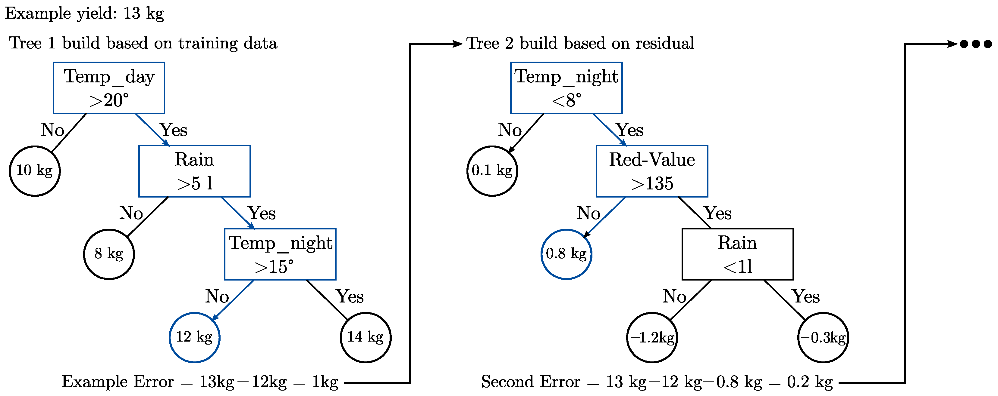
A tree ensemble is a family of regression trees where the final prediction is the sum of the predictions for each tree. The appropriate tree ensemble is learned from training data by iteratively adding new trees into the given ensemble that maximize the prediction performance of the trees already in the ensemble plus the new tree that has to be added. Maximizing the prediction performance is performed by minimizing the residuals, i.e., the difference between the observed true values of the training samples and the estimated values of the tree ensemble. In other words, for a given tree ensemble E k of k trees and its residuals, a new tree e k + 1 that fits best to these residuals is combined with the given ensemble E k , which produces the boosted version E k + 1 of E k . This is performed for k ( 1 k K ) iterations, until the residuals have been minimized as much as possible. Figure 1 depicts an illustrative example from the application field of yield prediction.

2.2. Shapley Values for Feature Attributions

The Shapley value is capable of attributing resources in a cooperative game fairly among players. A cooperative game ( P , v ) consists of a finite set of players P = { 1 , 2 , , p } and a value function v : 2 P R that assigns a value to each subset (coalition) of players, with 2 P being the powerset of P. The Shapley value represents the average contribution of a player in all possible coalitions. The Shapley value φ i ( v ) for a player i and a value function v is defined as follows:
φ i ( v ) = S P { i } | S | ! ( p | S | 1 ) ! p ! ( v ( S { i } ) v ( S ) ) .
The fraction is made by permuting the set of players and averaging the difference when evaluating the value function over the coalition S with all players that precede a player i in the given order with and without i itself. The number of players preceding in the formula coincides with the number of players in the set S, having S ! possible orders. Similarly, players who succeed i have ( p | S | 1 ) ! possible orders. Normalizing with all possible p ! permutations results in the factor in Equation (1).
It is important to note that the Shapley value is the only attribution score for cooperative games that satisfies the four game-theoretic properties of efficiency (i.e., the sum of the Shapley values of all players equals the value of the grand coalition), symmetry (i.e., equal scoring of players that contribute equally to all possible coalitions), dummy variables (i.e., the score of a non-relevant player is zero), and additivity (i.e., combined predictions (e.g., by a random forest R) result from adding (and averaging) the individual scores (e.g., of the trees of R).
Shapley values are further leveraged to obtain explanations in machine learning models. We assume that a dataset X R n × m with targets y R m is divided into data for training and testing a machine learning model M. In this context, we interpret the set of players P and the value function v for feature attributions. The definition of the players P is simple, as we want to attribute a score to each feature f 1 , , f n , so P = { f 1 , f n } . The value function v will be defined for a model M and a data point x that we want to explain, so we will write v M , x . The input of the function will be a set of features S P .
In general, two families of value functions are considered in the literature, conditional value functions and interventional value functions. Conditional value functions define the expected conditional output of the model at a data point, assuming that only the features of S are known to the model, as follows:
v M , x ( S ) = E M ( X ) X S = x S .
Interventional value functions are motivated by causal inference. They simulate an intervention on the features not in S, denoted as S ¯ , by modeling a distribution D from the product of the marginal distributions of the features in S ¯ , as follows:
v M , x ( S ) = E D M x S , X S ¯ .
We note that this definition of a value function allows the simulated features of S ¯ to break with the correlations with the features of S, finally leading to unpredictable model behavior.
When looking at applications of Shapley value feature attributions, the value function is used to determine the prediction of the model when only a subset of features can be accessed.
For a simple example, we can look at a problem where the feature space consists of two temperature measures of the same day, and we try to predict the temperature of the following day. Naturally, in this scenario, the two features are somehow correlated, as the temperature can only vary so much during one day. The question of choosing a value function now becomes the question of giving estimates of the model behavior when one of the measurements is missing. When choosing a conditional value function, we need to estimate the model output directly without missing information. Although there is no general solution to this problem, we propose a solution for the concept of random forests in Section 2.4. For an interventional value function, we do not estimate the model output, but estimate the feature value and then use the new fully reconstructed data point to obtain a model prediction. From an application-driven point of view of feature selection, interventional value functions are problematic because of the difficulties of modeling distributions, as it has to be done to estimate the missing feature value from the remaining features of a subset. In our example, when one of the measurements is unknown, for an interventional value function, we need to simulate its value. That could, for example, result in merging measurements that are taken from different seasons and show a wider difference than naturally possible in our dataset, breaking the natural correlations of the data. Finally, this leads us to evaluating the model at a data point that is not in the training distribution, where, especially for random forests, the model behavior is unpredictable.

2.3. Selecting a Value Function

The selected value function is integral in the successful use of the Shapley values for feature selection. We define conditions to define a value function that enables Shapley value feature attributions to be well suited for feature selection. The conditions are based on a recent criticism of the Shapley values [45,46,47,48] and avoid problems that the respective works have uncovered. While the four mentioned works [45,46,47,48] regarding this topic focus on defining a value function for Shapley values that will cause negative examples when applied as a tool for feature selection, we take learnings from their counterexamples and extract necessary conditions for defining the Shapley value in a way that they can be used for feature selection. A detailed description of the problems and solutions will be given below. Following the presented conditions will result in a value function well suited for feature selection and explainability on regression trees. The conditions are as follows:
C1: The value function must not be interventional. The negative effects of interventional value functions for the Shapley values in explainability and feature selection are examined by Kumar et al. [45]. As explained above, an interventional value function will break down with the correlations within the dataset. This will force the value function to evaluate the model M at data points outside the distribution of training data. This can lead to unexpected model behavior, especially for random forests.
C2: The value function should correctly attribute relevant and irrelevant features. Huang and Marques-Silva [46] create a value function that allows a Shapley value feature attribution to attribute no value to features that are important for model prediction. In the same scenario, features that are not important to the model output receive a non-zero attribution value. The choice of a value function to utilize Shapley values for feature selection should avoid these problems.
C3: The value function should consider multiple different training data points when estimating the expected conditional answer of the model. This property is important, since it prevents the evaluation of the value function v M , x ( S ) to only consider data points where the values of the features in the set S match the values of x. As Sundararajan and Najmi [47] point out, this can cause problems when the data point x is unique within the dataset. This leads to the value function always estimating the model output based on the output of a singular data point and, subsequently, v M , x ( S ) = v M , x ( T ) for all S , T P , making it impossible to distinguish important features.
C4: The value function should allow the calculation of Shapley value feature attributions in polynomial time. The problem of Shapley value calculation is known to be NP-hard. As the number of features can be high, especially when we consider the task of feature selection, the calculation should be feasible in a moderate time frame. Although there exist approximation techniques for the Shapley value calculation [49,50] that can improve the computational complexity, they add a layer of uncertainty that needs to be considered.

2.4. A Value Function for Random Forests

To define the value function, we want to evaluate the conditional expected answer of a random forest for a data point x. Generally, a random forest is built from multiple binary regression trees.
For simplicity, we will describe the conditional value function v M , x ( S ) for the model M to be just one singular binary regression tree given access to only a limited number of features S. For a random forest consisting of multiple trees, we just have to repeat the procedure and to add the results.
  Therefore, we now assume the following:
  • The model M is a singular binary random tree given access to only a limited amount of features S.
  • Each interior node of M consists of a feature f that is used for the test, a threshold t that indicates at what threshold to split for the feature F at the according node into the left or right child node.
  • Each leaf node shows its output value v a l .
  • Each node also shows its cover C, i.e., the number of training data points that reach this node when traversing the tree.
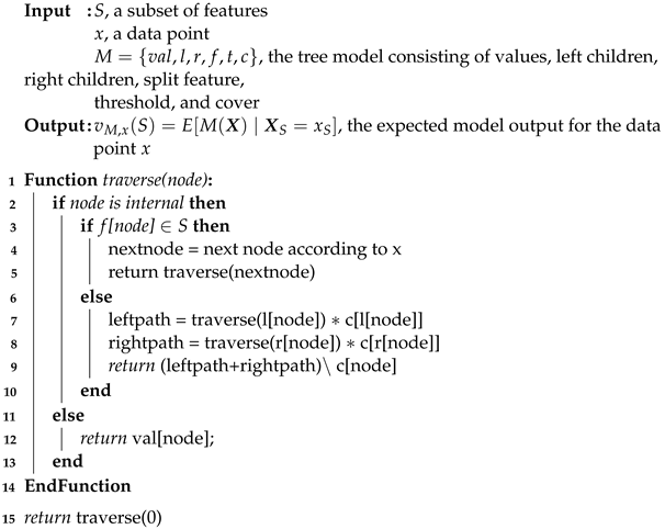
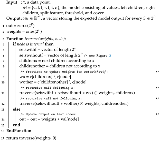
To evaluate v M , x ( S ) , we have to traverse the tree, starting at the root node. At each interior node, we check whether the feature f is in the set S. If this is the case, we continue to traverse the tree, according to the value of feature f from the data point x. This is since we assume that the features of x in S are known. If the feature f is not in S, we need to estimate the expected model output according to the distribution of the training data. In this case, we will continue to traverse the tree down both child nodes, with the final evaluation of v M , x ( S ) being the weighted sum of both continuations. The weights are determined by the fractions of training data points that flow down the regarding paths, calculated by the cover values of the nodes.
This traversal procedure was first described by Lundberg et al. [12] and can be calculated using the recursive Algorithm 1. For the algorithm, we assume the model M to be a single binary tree.
Algorithm 1: Conditional value function v M , x ( S ) for a regression tree M.
Geomatics 04 00016 i001
The defined value function has all the properties explained above.
  • C1: The function is conditional and not interventional.
  • C2: When considering features relevant to the model, we can define a relevant feature as a feature capable of altering the model output. When a feature f is capable of altering the model output, there exists at least one node within the tree that splits on the value of f. Therefore, our value function will give a different result when evaluated on the sets S P { f } and S { f } , giving a non-zero marginal contribution and, finally, a non-zero attribution of the feature. Similarly, features that are not relevant and are not considered as split feature in any node within the tree will never obtain a non-zero marginal contribution and will receive no feature attribution.
  • C3: The value function will consider multiple training instances when estimating the conditional expected answer of the model, as long as at least one relevant feature f is missing from the set S. If a relevant feature is missing, at least two branches of the tree are followed during the estimation of the expected answer of the model M. Both branches represent at least one data point in the training data following the path, as otherwise, no split at the feature f would have been possible.
  • C4: The calculation of the Shapley value feature importance is possible in polynomial time, as stated by Lundberg et al. [12] for the classical definition of Shapley values and extended by Huber et al. [51] for groups of features.

3. The Problem of Model Averaging

In the previous section, we explain how Shapley values must be utilized for a successful feature selection. In this section, we discuss a weakness of Shapley values for feature selection, which cannot be fixed by the choice of the value function. To evaluate the impact of model averaging, we give an algorithm that uses the conditional value function defined above to perform feature selection without suffering from model averaging.

3.1. Axiomatic Problems of the Shapley Value for Feature Selection

Even with a carefully selected value function, a feature selection based on Shapley values cannot be optimal. The nature of Shapley values for feature selection as a model averaging procedure includes measuring the impact of a feature on every possible subset of features, as can be seen in Equation (1). What is model averaging?
In feature selection for prediction models, it is uncertain which features should be considered for the final feature selection. Model averaging is the process of quantifying the influence of all features with respect to the predictions [52,53]. Shapley value feature selections are a model averaging procedure by definition, as Shapley value feature attributions are calculated by considering all possible subsets of features during the calculation of the Shapley value of every singular feature. This results in features that are not in the optimal feature selection that can alter the feature selection process.
For example, we can assume a scenario with two features, f 1 and f 2 , that explain the data well when selected together but poorly when selected alone. When calculating the feature attribution for the feature f 1 , the importance will not be correctly reflected, since, for every set S within Equation (1) that does not include the feature f 2 , the marginal contribution when adding f 1 will be low! This results in a Shapley value feature selection that might not select the features f 1 and f 2 , even though their actual prediction capabilities are high, leading to a non-optimal selection. A real-world example of this behavior is explained in Section 4.2.

3.2. Conditional Feature Selection

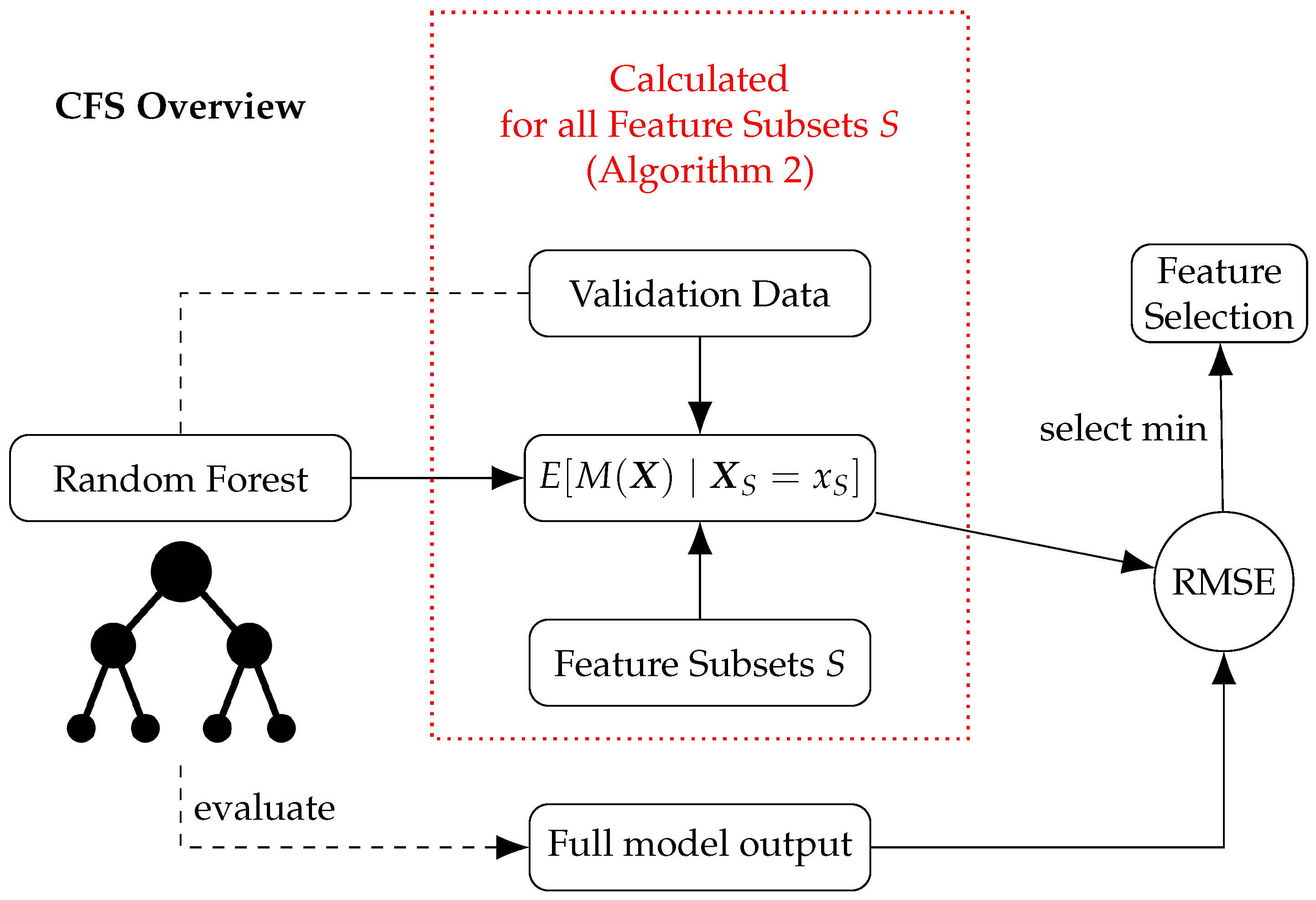
As a solution to the above problem, we present an algorithm called Conditional Feature Selection(CFS) that allows us to evaluate a feature selection S without considering the features not in S, by simply traversing the decision tree, once. A visual summary of the procedure is shown in Figure 2. Since we will update the estimated model answer for all possible subsets simultaneously, we start by allocating memory for the output of all possible 2 n sets S by creating a vector o u t R 2 n . Each set S corresponds to exactly one entry in o u t , and the vector will be used to synchronize the results of multiple recursive calls of the t r a v e r s e method, each ending in a different leaf. A possible correspondence of the feature subsets with an ordering in the vector can be found in Figure 3. Furthermore, we use a vector w e i g h t s R 2 n with the same correspondence to the sets S to store weights that are unique for every path of the tree. The weights determine to what extent the value of the path leaf contributes to v M , x ( S ) . Following a path and splitting at a node n with a feature f, for a set S, we observe three cases to update the weight. First, when f S and we follow the path according to the value of f in x, the weights remain the same. Second, when f S and we follow the path not according to the value of f in x, the weights are multiplied by 0. Third, when f S , we need to estimate the behavior of the model based on the fraction of training data points that follow both branches of the path, determined by the cover of the node n and both children. For the following algorithm, we assume pre-processing to generate the lists s e t s w i t h f and s e t s w i t h o u t f for each feature f. s e t s w i t h f has the value 1 when f S for the set S that corresponds to the same spot in o u t and the value 0 otherwise. s e t s w i t h o u t f has the value 1 when s e t s w i t h f has the value 0 at the same spot and the value 0 otherwise. An example of the two vectors is shown in Figure 3. When working with vectors, ∗ is the scalar multiplication and ⊙ is the element-wise multiplication.
We can now use this algorithm to find the best selection of features S for a given criterion. This can be a maximum number of features k to be selected or a maximum deviation allowed from the model output given the full set of features. To find the best feature selection, we divide a validation set V R n × m v from our training data X R n × m with targets y _ v a l R m v . The goal of our feature selection will be to find the selection S that minimizes the error between the output of the full model M and the expected output of the model v M , x ( S ) for the data points in the validation set. To measure this error, we use the Root Mean Squared Error (RMSE) as follows:
RMSE ( y ^ , y ˜ ( S ) ) = MSE ( y ^ , y ˜ ( S ) ) = 1 m v i = 1 m v y ^ i y ˜ i ( S ) 2 ,
where y ^ is the output of the full model M on the validation set and y ˜ ( S ) is the expected answer of the model M when only the features in S are known, as it is calculated in Algorithm 2. The whole process is shown in Figure 2.
Algorithm 2: Conditional value function for all S.
Geomatics 04 00016 i002

3.3. Runtime Analysis

The runtime of Algorithm 1 is analyzed in [12]. The complexity of a single execution of the algorithm is proportional to the number of leaves l in the respective tree. For our use case, we need to analyze every individual feature subset of the 2 P possible feature subsets. For an ensemble of k trees, we need to repeat this procedure k times, leaving us with a runtime of O ( k l 2 P ) . Although this runtime is still exponential in the number of features, Lundberg et al. [12] propose an algorithm for Shapley value calculation in polynomial time for random forests.
Algorithm 2 only needs one execution per tree, since every subset value is updated simultaneously. In this algorithm, the element-wise multiplication in lines 12 and 13 to update the weights is the most costly part, since all 2 P subsets are updated. The number of updates is again proportional to the number of leaves in a tree, and we need to perform this procedure for every tree in the ensemble, again leaving us with a runtime of O ( k l 2 P ) . For practical applications, it is beneficial that the most expensive part of the algorithm is the element-wise multiplication of two vectors, as this is a common problem and offers multiple ways of efficient implementation using GPU acceleration [54,55].
It is not possible to improve the runtime of CFS by applying the same idea as for the fast calculation of the Shapley values. The main concept is to iteratively update the calculated Shapley values when traversing the tree, removing the need to track the value function for every existing subset of players. However, for CFS, we are relying on tracking the change in every subset, making a runtime of O ( k l 2 P ) the best we can reach.

3.4. CFS Example

To further increase the understanding of the differences between the CFS algorithm as an exhaustive feature selection tool and the Shapley values as a heuristic approach, we present an example. We use Algorithm 2 to compare CFS and Shapley value feature selection for the example shown in Figure 4. For better readability, we omit the brackets for the feature sets and write F 12 for { F 1 , F 2 } . After the first call of traverse, we will only track the next recursive function calls for the internal nodes or the update of the output for leaf nodes. First, we initialize the following:
all subsets= [ , F 1 , F 2 , F 12 ]
setsWithF1= [ 0 , 1 , 0 , 1 ]
setsWithoutF1= [ 1 , 0 , 1 , 0 ]
out= [ 0 , 0 , 0 , 0 ]
weights= [ 1 , 1 , 1 , 1 ]
Algorithm 2 starts with traverse([1,1,1,1], K1). According to the data point x, we would follow the right path in the tree towards node K3. This determines childrenx and childrenother in lines 7 and 8 of Algorithm 2. The two weights are then updated according to the cover of the two nodes in lines 9 and 10. For both children, we start the next recursive call of the algorithm.
split feature= F 1
childrenx=K3
childrenother=K2
wx= 80 / 100
wother= 20 / 100
recursive call: t r a v e r s e ( ( [ 0 , 1 , 0 , 1 ] + [ 8 10 , 0 , 8 10 , 0 ] ) [ 1 , 1 , 1 , 1 ] , K 3 ) [1]
Update with full weight when F1 is known and partial weights when not
recursive call: t r a v e r s e ( [ 2 10 , 0 , 2 10 , 0 ] [ 1 , 1 , 1 , 1 ] , K 2 ) [2]
Update with zero weight when F1 is known and partial weights when not
  • [1] t r a v e r s e ( ( [ 8 10 , 1 , 8 10 , 1 ] ) , K 3 )
recursive call: t r a v e r s e ( ( [ 0 , 1 , 0 , 1 ] + [ 5 8 , 0 , 5 8 , 0 ] ) [ 8 10 , 1 , 8 10 , 1 ] , K 7 ) [3]
recursive call: t r a v e r s e ( [ 3 8 , 0 , 3 8 , 0 ] [ 8 10 , 1 , 8 10 , 1 ] , K 6 ) [4]
  • [3] t r a v e r s e ( ( [ 1 2 , 1 , 1 2 , 1 ] ) , K 7 )
out= [ 0 , 0 , 0 , 0 ] + [ 1 2 , 1 , 1 2 , 1 ] 4 = [2,4,2,4]
The value 4 of leaf K7 is added to the output
The weights reflect that the value is added fully for sets including F1
For sets not including F1 1 2 of training examples reach K7
  • [4] t r a v e r s e ( ( [ 3 10 , 0 , 3 10 , 0 ] ) , K 6 )
out= [ 4 , 2 , 4 , 2 ] + [ 3 10 , 0 , 3 10 , 0 ] 3 = [ 29 10 , 4, 29 10 , 4]
The value 3 of leaf K6 is added to the output
The weights reflect that no value is added for sets including F1
For sets not including F1 3 10 of training examples reach K6
  • [2] t r a v e r s e ( ( [ 2 10 , 1 , 2 10 , 1 ] ) , K 2 )
recursive call: t r a v e r s e ( ( [ 0 , 0 , 1 , 1 ] + [ 1 2 , 0 , 1 2 , 0 ] ) [ 2 10 , 0 , 2 10 , 0 ] , K 5 ) [6]
recursive call: t r a v e r s e ( [ 1 2 , 1 2 , 0 , 0 ] [ 2 10 , 0 , 2 10 , 0 ] , K 4 ) [7]
  • [6] t r a v e r s e ( ( [ 1 10 , 0 , 2 2 , 0 ] ) , K 5 )
out= [ 29 10 , 4 , 29 10 , 4 ] + [ 1 10 , 0 , 2 10 , 0 ] 2 = [ 31 10 , 4, 33 10 , 4]
The value 2 of leaf K5 is added to the output
When F1 is known, K5 is never reached and no value is added
  • [7] t r a v e r s e ( ( [ 1 10 , 0 , 0 , 0 ] ) , K 5 )
out= [ 31 10 , 4 , 33 10 , 4 ] + [ 1 10 , 0 , 0 , 0 ] 1 = [ 32 10 ,4, 33 10 ,4]
The value 1 of leaf K4 is added to the output
Only when F1 and F2 are unknown the path is followed to add value
The result [ 32 10 , 4, 33 10 , 4] can now be directly interpreted as the expected output of the model M for the data point x when we only assume access to the information in the subsets of features [ , F 1 , F 2 , F 12 ] . In the case of this model, we see that the answer when only F1 is known is the same as when both F1 and F2 are known. In general, the idea of CFS is to find the combination of features that minimizes the difference between the expected model answer for the feature subset and the output of the full model. We see that the main contribution to the runtime comes from the element-wise multiplication ⊙. For n features, the operation adds 2 n multiplications per weight update, growing exponentially in the number of features. We can now use the obtained values to calculate the following Shapley values ϕ F 1 and ϕ F 2 :
φ F 1 ( v ) = 1 2 ( 4 33 10 ) + 1 2 ( 4 32 10 ) = 0.75
φ F 2 ( v ) = 1 2 ( 4 4 ) + 1 2 ( 33 10 32 10 ) = 0.05
In this case, the Shapley values hint towards the same selection as CFS, as ϕ 1 ( v ) reveals the higher impact of feature F1 on the model output. We saw in the previous example that the evaluation of the expected model output for decision trees makes it necessary to track 2 n weights for every path in the tree. Shapley values can be calculated by only tracking 2 n values for every path, since each path has a positive and a negative contribution to the calculation of the Shapley value according to Lundberg et al. [12]. The contribution is positive for every occurrence of the path in the calculation of v ( S i ) in Equation (1). To occur in this calculation, the path must be as indicated by the example x on every split that includes the feature Fi. First, we calculate φ F 1 . We do so by listing the positive and negative impacts on the final Shapley value of every path of the model, represented by the leaf node the path ends in as follows:
K4:pos=0 K5:pos=0
neg= 1 2 2 10 1 2 neg= 1 2 20 100 10 20 + 1 2 2 10
φ F 1 = 0 1 20 1 φ F 1 = 1 20 3 20 2
K6:pos=0 K7:pos=1
neg= 3 10 neg= 5 10
φ F 1 = 7 20 3 10 3 φ F 1 = 25 20 + ( 1 1 2 ) 4 = 0.75
Now for φ F 2 , first, we note that the paths ending in K6 and K7 have no impact on φ F 2 , as the feature does not appear within the paths, and thus the positive and negative contributions on the Shapley value will always be equal. We note the following remaining paths:
K4:pos=0 K5:pos= 1 2 0 + 1 2 2 10
neg= 1 2 1 10 + 1 2 0 neg= 1 2 2 10 10 20 + 1 2 0
φ F 2 = 0 1 20 1 φ F 2 = 1 20 + ( 1 10 1 20 ) 2 = 0.05
We note that, for the example, the amount of calculations needed for both problems is roughly the same, as we have only two features. However, the Shapley value calculation for random forests will scale linearly in the number of features, while CFS will scale exponentially.
In summary, we now discuss two different procedures for feature selection. On the one hand, we have a heuristic feature selection approach by using Shapley values as a model averaging procedure. On the other hand, we introduce CFS as an exhaustive feature selection tool to avoid model averaging. However, with respect to runtime, we will see that Shapley value feature selection outperforms CFS for random forests. We will now evaluate both procedures in an experimental setting featuring real-world problems from the field of geomatics.

4. Experiments

In this section, we evaluate three different options to select features to preserve model performance in well-known real-world geomatics datasets. As a baseline and representation of the state of the art, we use the internal Gini feature importances of random forests. We show how a greedy selection of features by Shapley value feature importances improves over the state of the art and evaluate the impact of model averaging by discussing the results of the CFS algorithm. First, we give an in-depth explanation of a selected real-world example that highlights the differences between CFS and greedy Shapley value feature selection. Following this, we show the results of further experiments on different datasets.

4.1. Experimental Design

To evaluate the three different feature selection methods and to build our base model M, we use the popular eXtreme Gradient Boosting (XGBoost) [43] to build a random forest. XGBoost builds the trees sequentially, where each tree is designed to reduce the residual error of the already-existing ensemble. For hyperparameter tuning, a Tree-Structured Parzen Estimation (TPE) [56] is applied. This is a sequential model-based optimization approach. Models are constructed sequentially to approximate the performance of the model for a set of hyperparameters based on historical measurements. TPE estimates the underlying relations between a quality measure and the hyperparameters by exposing the underlying expression graph of how a performance metric is influenced by the hyperparameters. For this study, the Python implementation of TPE within the Optuna framework is used to tune the hyperparameter for each selection of subsets [57] and run for 25 iterations without any additional pruning involved to optimize accuracy in a fivefold cross-validation of the training data.
The three different feature selection methods evaluated are implemented as follows: First, we use the internal Gini feature importances of the random forests as a baseline and representation of the most used feature selection methods in practical applications. The feature selection is performed by greedily selecting the highest scoring feature according to the internal feature importance from XGBoost as a baseline selection. To calculate the internal Gini feature importance for a feature, we evaluate all splits made with the help of the features. The Gini entropy is calculated according to the amount of training data that are divided by the split, and lastly, all are added up. As a second approach, we evaluate the feature selection achieved by greedily selecting the feature with the highest absolute Shapley value in each iteration. This method represents the core question of our manuscript, whether Shapley values can be used for feature selection in such a fashion. Lastly, we have our novel approach of CFS that can be seen as a way of using the idea of Shapley values for feature selection, without suffering from model averaging, and thus can be used to evaluate the impact of model averaging on different datasets and raise our understanding of the problem. We perform our experiments by selecting a subset of every size with each of the three feature selection methods. We then optimize and train a new model on the subset of features to report the resulting accuracy on the testing data. With this procedure, good feature selections should result in high accuracy and low prediction error, giving us a ranking of the feature selection processes.

4.2. Explaining Model Averaging on a Real-World Problem

We start our experimental evaluation by taking a more in-depth look at a real-world problem to understand the conditions that cause model averaging to be a problem for Shapley value feature selection. We use the bike rental dataset from the UCI machine learning repository [58]. The dataset is often investigated within the literature [59] and has many advantages in explaining feature selection. Most importantly, we can understand the problem and the features involved. The target variable is the number of bikes rented in an hour through the Capital Bikeshare system in Washington DC, USA. The features we use are described in Table 2. We choose this dataset to discuss model averaging since its features have interesting relations. The feature year is important without considering any other feature, since the values for 2013 are generally higher than those for 2012. The mean for all data points in 2012 is 143 bikes rented, and for 2013, it is 234 bikes rented. The features of holidays, weekdays, and workdays also have an interesting relationship with each other. The weekday and holiday features can be used to reconstruct the workday feature, since a workday is a day not on the weekend, where no holiday occurs. Finally, we see a strong correlation between temperature and perceived temperature, with a Pearson correlation coefficient of 0.988.
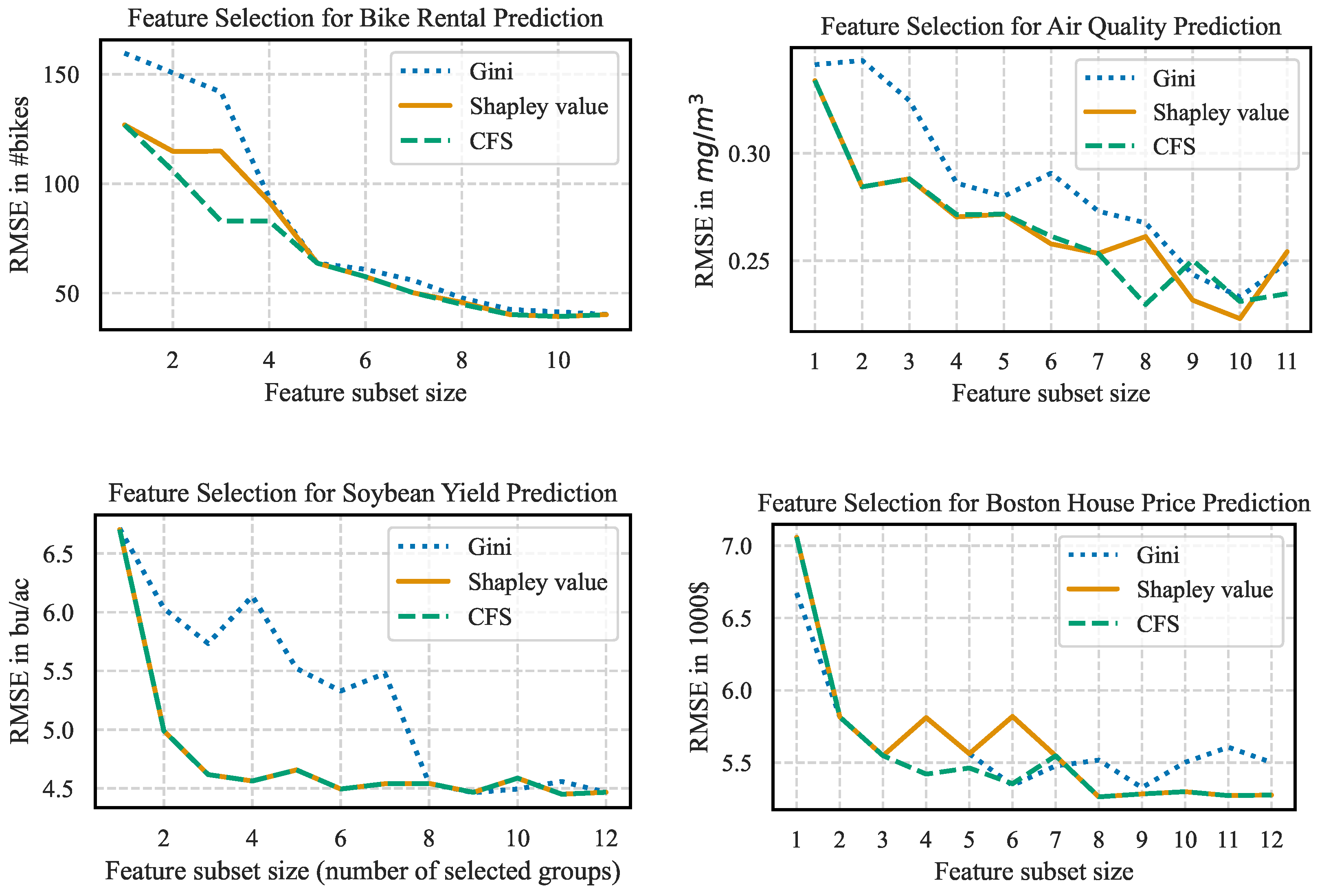
For this dataset, we select subsets of all sizes from 1 to 11 with three different selection procedures. In the analysis, we especially focus on the difference between the Shapley value feature selection and CFS. The results are shown in the top-left graph of Figure 5. Differences occur for selections of sizes 2, 3, and 4. The Shapley value feature selection for size 2 consists of the features year and hour, while CFS selects temperature and hour. While the hour is the same in both selections, we are able to see a problem with model averaging for the Shapley value feature selection. This is because the feature year is important when adding it to any subset of features, which is good for achieving a high Shapley value. However, the feature temperature is more important to estimate the number of bikes rented. This can be specified by training a simple linear regression on the features temperature and year, exclusively. Although the regression for year has an RMSE of 176 bikes, the temperature-based regression only has an error of 167 bikes. The temperature variable is selected later by the Shapley value feature selection, since sets that already include the highly correlated perceived temperature lower the Shapley value feature attribution and delay the selection of an important feature. This shows how model averaging can be problematic.
For the feature selection of size 3, the Shapley value feature selection method selects the feature temperature next. The CFS algorithm adds the feature workday to the feature selection. Again, due to model averaging, the Shapley value feature selection does not select the best feature, as year again adds value to every possible subset, but the feature workday is not yet chosen due to the relations to the other features weekday and holiday. Therefore, for a selection of size 3, both approaches include the features temperature and hour. Understanding why adding the feature workday is advantageous only is possible when considering the whole situation, including the feature relations, as a linear regression model trained on workday alone has the highest error of all features with an RMSE of 182 bikes. However, CFS reveals that combining the three features in a random forest allows the RMSE to drop from 106 to 83 bikes by including the feature. For subsets of size 4, both approaches add the feature rush hour to the selection, still inheriting the problems of the previous selection. From now on, both approaches add the same features to the selection. Furthermore, both approaches consistently beat the Gini feature importance in terms of RMSE.

4.3. Further Experiments

We solidify our results by performing more experiments on two datasets taken from the well-known UCI machine learning repository and an additional application from soybean yield prediction with an extended feature space. The experimental setup is the same as explained in Section 4.1. The first additional dataset we analyze is about the prediction of air quality [60]. The dataset consists of 9358 instances consisting of 12 features that can be used to estimate the hourly CO concentration measured in mg/m3 in an Italian city. The second experiment carried out within our work is the prediction of house prices in Boston [61]. Here, the dataset consists of 505 data points from the year 1970, where 13 variables describe features of the house and the corresponding neighborhood. The target price is the price of the house in USD 1000. Lastly, we include a dataset with a more extensive feature space to predict soybean yield in b u / a c within the United States. One b u / a c is the same as 0.0673 t/ha. The dataset is the same as described in [62], and we focus on the prediction of the yields in the year 2022. The 1129 input features consist of different measurements extracted from remote sensing satellite observations and handcrafted features. For our analysis, the features are grouped according to the satellite sensors used for data acquisition, together with one group for all hand-crafted features, resulting in 13 different groups that can be selected during the feature selection process. To calculate the Shapley values, we use the extension of Shapley values for groups of features as it is introduced in [51] and use a similar extension for our CFS algorithm.
We can use the results of the experiments to gain more insight about the model averaging problem and the connected strength to mitigate model averaging with CFS. For model averaging to become problematic in Shapley value feature selection, we need two conditions to be met. First, we need to find two or more features that are correlated or contain similar information. Second, we need a different feature that has fewer capabilities when used within a prediction model but is mostly unrelated to the rest of the dataset. Due to the Shapley value feature importance being averaged over the marginal contribution to every feature subset, the Shapley value of the features with similar information is lowered every time they are added to a subset where the other features are already present. This finally results in the feature that is mostly unrelated to the rest of the dataset but with lower prediction capabilities to be selected first. Taking this insight, we can analyze the results in the air prediction dataset on the top-right corner of Figure 5. The selection from Shapley value feature selection and CFS is mostly the same, with the first distinction being made for feature subsets of size 8. This is because the seven most important features for the prediction problem are all highly correlated with each other, with absolute Pearson correlation coefficients above 0.9. The first difference in selection occurs when the previously described conditions are met. The features relative humidity and temperature are highly correlated with a Pearson correlation coefficient of −0.77, while the feature absolute humidity is left to select with all correlations within the dataset being lower. CFS is able to correctly attribute higher prediction capabilities of relative humidity, while the correlation with the temperature hinders the Shapley value feature selection from doing so. For soybean yield prediction, we see that CFS and Shapley value feature selection produce identical feature subsets. This can be explained by using groups of features in this example, where highly correlated features can only be selected as a whole group. In this scenario, it is very unlikely that the remaining feature groups contain similar information, and model averaging is not a real issue for this dataset, resulting in CFS and Shapley value feature selection being equally potent. Lastly, we have the Boston house price prediction dataset where, again, the first feature selections are the same. A change occurs for the fourth selected feature where CFS selects a feature describing the amount of nitrogen oxides in the air that is highly correlated with two other features, the amount of industry in the area and the average distance to the next Boston employment centers, finally leading to Shapley value feature selection providing different results. In summary, the experiments show how different correlations within the dataset can hinder Shapley values to find the optimal selection of features based on features that are not part of the optimal selection of a given size.
Throughout all experiments, we observe similar behavior of the three different feature selection approaches. Looking at the averaged RMSE values for all possible subset sizes in Table 3, we see that the Shapley value feature selection approach and CFS are always very close together in terms of accuracy, with the CFS algorithm having a small advantage for every dataset but for the soybean yield prediction, where the two approaches produce identical feature subsets. On the same note, we see greedy feature selection according to the internal Gini feature importances, which performs significantly worse for all our datasets, when compared with the other approaches. A detailed illustration of the results in Figure 5 shows the same picture as the table. The green and orange lines, showing the results for CFS and Shapley value feature selection, respectively, are always very close together, with the blue line showing the results of the internal Gini feature importances mostly lying above the other two approaches.

4.4. Runtime Experiments

The computational complexity and subsequent runtimes are a crucial consideration when choosing which feature selection method to apply. After we have established a slight advantage in accuracy of the models trained on feature subsets selected by CFS, when compared with greedy Shapley value feature selection, we can take a deeper look into the runtimes. For real-life examples, we add the runtimes in Table 3 to calculate all Shapley values and to calculate the expected model output for every possible feature subset with CFS, given 1000 reference data points and 500 trees within our random forest. For the Boston house price dataset, we time the procedure for 500 reference data points and double the results for a fair comparison, as the dataset does not contain 1000 data points. We note that the Shapley value calculation with the algorithm in [12] can be performed in a matter of seconds, while we need multiple minutes to calculate CFS. The calculation times for the internal Gini importances are omitted, as they are calculated immediately after creating the trees. To further analyze the matter, we conduct another experiment. Without grouping features, our soybean dataset consists of 1129 features. We gradually restrict the dataset to contain only f features, with f [ 5 , 15 ] . As the performance of the prediction model is the first priority in this experiment, we use XGBoost to build a random forest with 100 trees, using the default parameters. In Figure 6, we plot the elapsed time in seconds as a function of the number of features and observe that the elapsed time grows exponentially in the number of features, which is indicated by the runtime in O ( k l 2 P ) . Further experiments indicate that the number of reference data points and the number of trees provide a linear scaling of the problem. Meanwhile, the runtime to calculate Shapley values on random forests remains at a few seconds, even for the entire dataset of 1129 features.

5. Discussion

Given a machine learning problem with a dataset and an existing model M, the subject of this article is the research question of whether Shapley values can be used as a tool to select a subset of features in a way that reduces the amount of input features and, therefore, the overhead in data acquisition, while the accuracy of the model M is conserved as much as possible. When approaching this question from a theoretical standpoint, we are able to formulate five possible challenges for Shapley value feature selection. Four of these challenges are exposed by related literature to the topic and are focused on constructing counter-exemplified examples for Shapley values as a feature selection tool by defining value functions that lead to the Shapley value feature selection to violate certain desired properties. The first contribution of our work is defining four conditions, C1 to C4, that need to be fulfilled by the value function, when Shapley values should be used for feature selection. We find that the conditional value function as defined in Algorithm 1 can satisfy all the conditions. The experiments carried out within Section 4 show that the resulting definition of Shapley values is indeed suitable for feature selection and outperforms the internal Gini feature importances of random forests as a benchmark, when both are used within a greedy feature selection algorithm. This is in line with other related works on the topic as presented in Section 1.2. The Shapley value feature importances are a better heuristic for the greedy feature selection, as the Gini importances focus only on the amount of training examples that are divided by a feature, but not directly on the impact on the target variable, when the feature is changed. This is the strength of Shapley values in machine learning and leads to a better quantification of the importance of a feature to the model and, therefore, to an importance score, well suited to select the most important feature to preserve the models’ performance on a subset.
However, we further analyze that there is a problem with Shapley values for feature selection that cannot be solved through the choice of the right value function. Shapley values, by definition, suffer from the problem of model averaging when they should be applied for feature selection. This means that the Shapley value of an individual feature is influenced by features that are not in the desired final selection, and the greedy selection according to Shapley values will be suboptimal. We introduce a novel approach, CFS, to isolate the impact of unselected features and measure the impact of model averaging in several real-world problems. The experiments, in general, support the existence of model averaging as a problem, where CFS outperforms Shapley value feature selection on all selected datasets, as shown in Table 3. An in-depth analysis of the different feature selections in the bike rental dataset in Section 4.2 shows that the correlation between features and, in particular, the possibility of reconstructing the feature values from one another is a crucial factor when model averaging hinders Shapley value feature importances to indicate the optimal selection of features. This conclusion is also supported by the soybean dataset, where similar features can only be selected as groups, and therefore, the respective groups cannot be reconstructed from the remaining ones. That being said, we need to note that the CFS algorithm is computationally expensive, when compared with Shapley values, at least for random forests, where Shapley values can be calculated in polynomial time. This suggests a research direction where the use of CFS is further explored.
Compared with other feature selection methods within the literature, first and foremost, we have to compare CFS with the Gini importance [22] as one of the most used feature importance measures for random forests. Its use comes from the integration into popular machine learning frameworks [63] together with the fast runtime, which allows constant evaluation within a machine learning project. However, we see that the fast runtime comes at the cost of accuracy, when we compare the reached accuracies for feature selections from greedy Gini feature selection with Shapley values and CFS within our experiments. On the other side of the spectrum of the trade-off from runtime and accuracy, we have a selection by a mean decrease in accuracy [64], where the random forest is retrained without a feature present, and the decrease in accuracy is attributed to the importance of the feature. While the evaluation for a singular feature with this method is very precise, it fails to acknowledge feature interactions. Here, Shapley value feature importances and CFS are advantageous, as they evaluate subsets of features and can therefore account for feature interactions. Lastly, we have to look at other approaches of using Shapley values for feature selection, like we established in the related work section of this manuscript. The biggest problem here is again the runtime of the approaches and the shortcomings regarding our defined necessary conditions for Shapley value feature selection, when we have to use a sample-based method to estimate the value function within Shapley value calculation, like it has to be performed for SHAP [8] or SAGE [14].
However, although CFS is formulated for random forests, the idea of evaluating the same value function as used in Shapley value calculation to minimize the error for feature selection can be transferred to other machine learning algorithms. For example, there exist Shapley value calculation procedures for deep learning applications. When exploring these options, the Shapley value calculation loses its advantage of fast calculations, as calculating Shapley values on arbitrary models remains NP-hard. Furthermore, restricting the number of subsets that should be considered for feature selection can further improve computational complexity and allow the evaluation of problems that include a larger feature space with CFS.
However, for the applications at hand, the improvements in accuracy that we were able to find with our experiments indicate that the trade-off between computational complexity and gained accuracy when circumventing the problem of model averaging hints at using Shapley values for feature selection for applied problems. Finally, the best solution is to be picked individually by deciding on a trade-off between accuracy and runtime, between CFS and Shapley values for feature selection, while both approaches are to be preferred over using the internal Gini importances of random forests for feature selection.

6. Conclusions

This study provides an in-depth analysis of the Shapley values for the selection of features for datasets from the field of geomatics. The topic of feature selection with Shapley values has been widely discussed within the field. On the one hand, we find many successful applications of the Shapley value for feature selection; on the other hand, we can find works describing the theoretical boundaries of the approach. Our contributions to the discussion with an application-driven study of Shapley values for feature selection can be summarized as follows:
  • The definition of four necessary conditions helps to define a Shapley value that can be used for selecting relevant features.
  • The model averaging problem is intrinsic to the definition of Shapley values. We provide CFS as an algorithm for feature selection without model averaging to allow for a quantitative evaluation of the impact of the problem.
  • The evaluation of CFS and Shapley values for feature selection in multiple real-world applications reveals a trade-off between runtime and accuracy when calculated on random forests.
In the future, we will build on our previous work [51] and further explore feature selection for predefined groups of features. This is crucial in contexts where multiple features are extracted from the same source, making it suboptimal to select only a subset from a single source. We will investigate more use cases for this approach, such as yield prediction. Another interesting research direction will be to improve the runtime of CFS, by either limiting the search space or applying sampling strategies. Additionally, we aim to explore a CFS approach motivated by the Shapley value definition within the SHAP framework. Using sampling of similar data points could estimate the model’s performance on a feature subset, thus removing the restriction of CFS to random forests, where Shapley value feature importance benefits from fast computing times.

Author Contributions

Conceptualization, F.H. and V.S.; methodology, F.H. and V.S.; software, F.H.; validation, F.H. and V.S.; data curation, F.H.; writing—original draft preparation, F.H. and V.S.; writing—review and editing, F.H. and V.S.; visualization, F.H. and V.S.; project administration, V.S.; funding acquisition, V.S. All authors have read and agreed to the published version of the manuscript.

Funding

This work was partially conducted within the project “Artificial Intelligence for Innovative Yield Prediction of Grapevine” (KI-iRepro). The project is supported by funds from the Federal Ministry of Food and Agriculture (BMEL) based on a decision of the Parliament of the Federal Republic of Germany. The Federal Office for Agriculture and Food (BLE) provides coordinating support for artificial intelligence (AI) in agriculture as a funding organization, grant number FKZ 28DK128B20.

Institutional Review Board Statement

Not applicable.

Informed Consent Statement

Not applicable.

Data Availability Statement

All data used within this research are publicly available and cited accordingly.

Acknowledgments

We thank Frank Schindler for the fruitful discussions and the proofreading of our manuscript.

Conflicts of Interest

The authors declare no conflicts of interest. During the preparation of this work, the authors used Writefull Premium in order to improve its readability. After using this tool/service, the authors reviewed and edited the content as needed and take full responsibility for the content of the publication.

References

  1. Van Klompenburg, T.; Kassahun, A.; Catal, C. Crop yield prediction using machine learning: A systematic literature review. Comput. Electron. Agric. 2020, 177, 105709. [Google Scholar] [CrossRef]
  2. Garg, A.; Mago, V. Role of machine learning in medical research: A survey. Comput. Sci. Rev. 2021, 40, 100370. [Google Scholar] [CrossRef]
  3. Akbari, M.; Do, T.N.A. A systematic review of machine learning in logistics and supply chain management: Current trends and future directions. Benchmarking Int. J. 2021, 28, 2977–3005. [Google Scholar] [CrossRef]
  4. Ali, A.M. Review of Artificial Intelligence Applications in the Geomatics Field. Int. J. Appl. Sci. Curr. Future Res. Trends 2023, 20, 1–12. [Google Scholar]
  5. Bordogna, G.; Fugazza, C. Artificial Intelligence for Multisource Geospatial Information; MDPI: Basel, Switzerland, 2022. [Google Scholar]
  6. Gao, S. Geospatial Artificial Intelligence (GeoAI); Oxford University Press: New York, NY, USA, 2021; Volume 10. [Google Scholar]
  7. Sheykhmousa, M.; Mahdianpari, M.; Ghanbari, H.; Mohammadimanesh, F.; Ghamisi, P.; Homayouni, S. Support vector machine versus random forest for remote sensing image classification: A meta-analysis and systematic review. IEEE J. Sel. Top. Appl. Earth Obs. Remote Sens. 2020, 13, 6308–6325. [Google Scholar] [CrossRef]
  8. Lundberg, S.M.; Lee, S.I. A unified approach to interpreting model predictions. Adv. Neural Inf. Process. Syst. 2017, 30, 4768–4777. [Google Scholar]
  9. Shapley, L.S. A value for n-person games. Contributions to the Theory of Games II; Kuhn, H.W., Tucker, A.W., Eds.; Annals of Mathematics Studies; Princeton University Press: Princeton, NJ, USA, 1953; pp. 307–317. [Google Scholar]
  10. Roth, A.E. The Shapley value: Essays in honor of Lloyd S. Shapley; Cambridge University Press: Cambridge, UK, 1988. [Google Scholar]
  11. Algaba, E.; Fragnelli, V.; Sánchez-Soriano, J. Handbook of the Shapley Value; CRC Press: Boca Raton, FL, USA, 2019. [Google Scholar]
  12. Lundberg, S.M.; Erion, G.; Chen, H.; DeGrave, A.; Prutkin, J.M.; Nair, B.; Katz, R.; Himmelfarb, J.; Bansal, N.; Lee, S.I. From local explanations to global understanding with explainable AI for trees. Nat. Mach. Intell. 2020, 2, 56–67. [Google Scholar] [CrossRef] [PubMed]
  13. Marcílio, W.E.; Eler, D.M. From explanations to feature selection: Assessing SHAP values as feature selection mechanism. In Proceedings of the 2020 33rd SIBGRAPI conference on Graphics, Patterns and Images (SIBGRAPI), Galinhas, Brazil, 7–10 November 2020; IEEE: Piscataway, NJ, USA, 2020; pp. 340–347. [Google Scholar]
  14. Covert, I.; Lundberg, S.M.; Lee, S.I. Understanding global feature contributions with additive importance measures. Adv. Neural Inf. Process. Syst. 2020, 33, 17212–17223. [Google Scholar]
  15. Zacharias, J.; von Zahn, M.; Chen, J.; Hinz, O. Designing a feature selection method based on explainable artificial intelligence. Electron. Mark. 2022, 32, 2159–2184. [Google Scholar] [CrossRef]
  16. Dhal, P.; Azad, C. A comprehensive survey on feature selection in the various fields of machine learning. Appl. Intell. 2022, 52, 4543–4581. [Google Scholar] [CrossRef]
  17. Venkatesh, B.; Anuradha, J. A review of feature selection and its methods. Cybern. Inf. Technol. 2019, 19, 3–26. [Google Scholar] [CrossRef]
  18. Chandrashekar, G.; Sahin, F. A survey on feature selection methods. Comput. Electr. Eng. 2014, 40, 16–28. [Google Scholar] [CrossRef]
  19. Huan, L.; Hiroshi, M. Feature Selection for Knowledge Discovery and Data Mining; Kluwer Academic Publishers: New York, NY, USA, 1998. [Google Scholar]
  20. Li, J.; Cheng, K.; Wang, S.; Morstatter, F.; Trevino, R.P.; Tang, J.; Liu, H. Feature selection: A data perspective. ACM Comput. Surv. (CSUR) 2017, 50, 1–45. [Google Scholar] [CrossRef]
  21. Huang, N.; Lu, G.; Xu, D. A permutation importance-based feature selection method for short-term electricity load forecasting using random forest. Energies 2016, 9, 767. [Google Scholar] [CrossRef]
  22. Menze, B.H.; Kelm, B.M.; Masuch, R.; Himmelreich, U.; Bachert, P.; Petrich, W.; Hamprecht, F.A. A comparison of random forest and its Gini importance with standard chemometric methods for the feature selection and classification of spectral data. BMC Bioinform. 2009, 10, 213. [Google Scholar] [CrossRef]
  23. Park, M.S.; Na, J.H.; Choi, J.Y. PCA-based feature extraction using class information. In Proceedings of the 2005 IEEE International Conference on Systems, Man and Cybernetics, Waikoloa, HI, USA, 10–12 October 2005; IEEE: Piscataway, NJ, USA, 2005; Volume 1, pp. 341–345. [Google Scholar]
  24. Jijón-Palma, M.E.; Amisse, C.; Centeno, J.A.S. Hyperspectral dimensionality reduction based on SAE-1DCNN feature selection approach. Appl. Geomat. 2023, 15, 991–1004. [Google Scholar] [CrossRef]
  25. Deng, H.; Runger, G. Feature selection via regularized trees. In Proceedings of the 2012 International Joint Conference on Neural Networks (IJCNN), Brisbane, Australia, 10–15 June 2012; IEEE: Piscataway, NJ, USA, 2012; pp. 1–8. [Google Scholar]
  26. Genuer, R.; Poggi, J.M.; Tuleau-Malot, C. Variable selection using random forests. Pattern Recognit. Lett. 2010, 31, 2225–2236. [Google Scholar] [CrossRef]
  27. Gazzola, G.; Jeong, M.K. Dependence-biased clustering for variable selection with random forests. Pattern Recognit. 2019, 96, 106980. [Google Scholar] [CrossRef]
  28. Alsahaf, A.; Petkov, N.; Shenoy, V.; Azzopardi, G. A framework for feature selection through boosting. Expert Syst. Appl. 2022, 187, 115895. [Google Scholar] [CrossRef]
  29. Shih, A.; Choi, A.; Darwiche, A. A symbolic approach to explaining bayesian network classifiers. arXiv 2018, arXiv:1805.03364. [Google Scholar]
  30. Arenas, M.; Barceló, P.; Romero Orth, M.; Subercaseaux, B. On computing probabilistic explanations for decision trees. Adv. Neural Inf. Process. Syst. 2022, 35, 28695–28707. [Google Scholar]
  31. Zhou, H.; Zhang, J.; Zhou, Y.; Guo, X.; Ma, Y. A feature selection algorithm of decision tree based on feature weight. Expert Syst. Appl. 2021, 164, 113842. [Google Scholar] [CrossRef]
  32. Dineen, J.; Kridel, D.; Dolk, D.; Castillo, D. Unified Explanations in Machine Learning Models: A Perturbation Approach. arXiv 2024, arXiv:2405.20200. [Google Scholar]
  33. Ribeiro, M.T.; Singh, S.; Guestrin, C. “ Why should i trust you?” Explaining the predictions of any classifier. In Proceedings of the 22nd ACM SIGKDD International Conference on Knowledge Discovery and Data Mining, San Francisco, CA, USA, 13–17 August 2016; pp. 1135–1144. [Google Scholar]
  34. Man, X.; Chan, E. The best way to select features? comparing mda, lime, and shap. J. Financ. Data Sci. Winter 2021, 3, 127–139. [Google Scholar] [CrossRef]
  35. Ribeiro, M.T.; Singh, S.; Guestrin, C. Anchors: High-precision model-agnostic explanations. In Proceedings of the AAAI Conference on Artificial Intelligence, New Orleans, LA, USA, 2–7 February 2018; Volume 32. [Google Scholar]
  36. Cohen, S.; Ruppin, E.; Dror, G. Feature selection based on the shapley value. Other Words 2005, 1, 155. Available online: https://www.ijcai.org/Proceedings/05/Papers/0763.pdf (accessed on 17 July 2024.).
  37. Cohen, S.; Dror, G.; Ruppin, E. Feature selection via coalitional game theory. Neural Comput. 2007, 19, 1939–1961. [Google Scholar] [CrossRef] [PubMed]
  38. Rozemberczki, B.; Watson, L.; Bayer, P.; Yang, H.T.; Kiss, O.; Nilsson, S.; Sarkar, R. The shapley value in machine learning. arXiv 2022, arXiv:2202.05594. [Google Scholar]
  39. Chu, C.C.F.; Chan, D.P.K. Feature selection using approximated high-order interaction components of the Shapley value for boosted tree classifier. IEEE Access 2020, 8, 112742–112750. [Google Scholar] [CrossRef]
  40. Fang, L.; Jin, J.; Segers, A.; Lin, H.X.; Pang, M.; Xiao, C.; Deng, T.; Liao, H. Development of a regional feature selection-based machine learning system (RFSML v1. 0) for air pollution forecasting over China. Geosci. Model Dev. 2022, 15, 7791–7807. [Google Scholar] [CrossRef]
  41. Strumbelj, E.; Kononenko, I. An efficient explanation of individual classifications using game theory. J. Mach. Learn. Res. 2010, 11, 1–18. [Google Scholar]
  42. Štrumbelj, E.; Kononenko, I. Explaining prediction models and individual predictions with feature contributions. Knowl. Inf. Syst. 2014, 41, 647–665. [Google Scholar] [CrossRef]
  43. Chen, T.; Guestrin, C. Xgboost: A scalable tree boosting system. In Proceedings of the 22nd ACM Sigkdd International Conference on Knowledge Discovery and Data Mining, San Francisco, CA, USA, 13–17 August 2016; pp. 785–794. [Google Scholar]
  44. Fournier-Viger, P. The Data Mining Blog: The KDDCup 2015 Dataset. 2016. Available online: https://data-mining.philippe-fournier-viger.com/the-kddcup-2015-dataset-download-link/, (accessed on 1 February 2022).
  45. Kumar, I.E.; Venkatasubramanian, S.; Scheidegger, C.; Friedler, S. Problems with Shapley-value-based explanations as feature importance measures. In Proceedings of the International Conference on Machine Learning, Virtual Event, 13–18 July 2020; PMLR: Breckenridge, CO, USA, 2020; pp. 5491–5500. [Google Scholar]
  46. Huang, X.; Marques-Silva, J. The Inadequacy of Shapley Values for Explainability. arXiv 2023, arXiv:2302.08160. [Google Scholar]
  47. Sundararajan, M.; Najmi, A. The many Shapley values for model explanation. In Proceedings of the International Conference on Machine Learning, Virtual Event, 13–18 July 2020; PMLR: Breckenridge, CO, USA, 2020; pp. 9269–9278. [Google Scholar]
  48. Fryer, D.; Strümke, I.; Nguyen, H. Shapley values for feature selection: The good, the bad, and the axioms. IEEE Access 2021, 9, 144352–144360. [Google Scholar] [CrossRef]
  49. Castro, J.; Gómez, D.; Tejada, J. Polynomial calculation of the Shapley value based on sampling. Comput. Oper. Res. 2009, 36, 1726–1730. [Google Scholar] [CrossRef]
  50. Castro, J.; Gómez, D.; Molina, E.; Tejada, J. Improving polynomial estimation of the Shapley value by stratified random sampling with optimum allocation. Comput. Oper. Res. 2017, 82, 180–188. [Google Scholar] [CrossRef]
  51. Huber, F.; Engler, H.; Kicherer, A.; Herzog, K.; Töpfer, R.; Steinhage, V. Grouping Shapley Value Feature Importances of Random Forests for Explainable Yield Prediction. In Proceedings of the Intelligent Systems Conference, Amsterdam, The Netherlands, 7–8 September 2023; Springer: Berlin/Heidelberg, Germany, 2023; pp. 210–228. [Google Scholar]
  52. Madigan, D.; Raftery, A.E. Model selection and accounting for model uncertainty in graphical models using Occam’s window. J. Am. Stat. Assoc. 1994, 89, 1535–1546. [Google Scholar] [CrossRef]
  53. Raftery, A.E. Bayesian model selection in social research. In Sociological Methodology; SAGE: Newcastle upon Tyne, UK, 1995; pp. 111–163. [Google Scholar]
  54. Okuta, R.; Unno, Y.; Nishino, D.; Hido, S.; Loomis, C. CuPy: A NumPy-Compatible Library for NVIDIA GPU Calculations. In Proceedings of the Workshop on Machine Learning Systems (LearningSys) in The Thirty-First Annual Conference on Neural Information Processing Systems (NIPS), Long Beach, CA, USA, 4–9 December 2017. [Google Scholar]
  55. Lam, S.K.; Pitrou, A.; Seibert, S. Numba: A llvm-based python jit compiler. In Proceedings of the Second Workshop on the LLVM Compiler Infrastructure in HPC, Austin, TX, USA, 15 November 2015; pp. 1–6. [Google Scholar]
  56. Bergstra, J.; Yamins, D.; Cox, D. Making a science of model search: Hyperparameter optimization in hundreds of dimensions for vision architectures. In Proceedings of the International Conference on Machine Learning, Atlanta, GA, USA, 16–21 June 2013; PMLR: Breckenridge, CO, USA, 2013; pp. 115–123. [Google Scholar]
  57. Akiba, T.; Sano, S.; Yanase, T.; Ohta, T.; Koyama, M. Optuna: A next-generation hyperparameter optimization framework. In Proceedings of the 25th ACM SIGKDD International Conference on Knowledge Discovery & Data Mining, Anchorage, AK, USA, 4–8 August 2019; pp. 2623–2631. [Google Scholar]
  58. Fanaee-T, H. Bike Sharing Dataset. UCI Machine Learning Repository, 2013. Available online: https://archive.ics.uci.edu/dataset/275/bike+sharing+dataset (accessed on 23 August 2023).
  59. Sathishkumar, V.; Cho, Y. Season wise bike sharing demand analysis using random forest algorithm. Comput. Intell. 2020, 40, e12287. [Google Scholar]
  60. Vito, S. Air Quality. UCI Machine Learning Repository, 2016. Available online: https://archive.ics.uci.edu/dataset/360/air+quality (accessed on 23 August 2023).
  61. Harrison, D.; Rubinfeld, D. Hedonic Prices and the Demand for Clean Air. 1978. Available online: https://www.cs.toronto.edu/delve/data/boston/bostonDetail.html (accessed on 20 November 2023).
  62. Huber, F.; Yushchenko, A.; Stratmann, B.; Steinhage, V. Extreme Gradient Boosting for yield estimation compared with Deep Learning approaches. Comput. Electron. Agric. 2022, 202, 107346. [Google Scholar] [CrossRef]
  63. Pedregosa, F.; Varoquaux, G.; Gramfort, A.; Michel, V.; Thirion, B.; Grisel, O.; Blondel, M.; Prettenhofer, P.; Weiss, R.; Dubourg, V.; et al. Scikit-learn: Machine Learning in Python. J. Mach. Learn. Res. 2011, 12, 2825–2830. [Google Scholar]
  64. Han, H.; Guo, X.; Yu, H. Variable selection using mean decrease accuracy and mean decrease gini based on random forest. In Proceedings of the 2016 7th IEEE International Conference on Software Engineering and Service Science (ICSESS), Beijing, China, 26–28 August 2016; IEEE: Piscataway, NJ, USA, 2016; pp. 219–224. [Google Scholar]
Figure 1. A snapshot of building a regression tree ensemble, where the second tree is chosen to minimize the residual value (i.e., true value − predicted value = 13 kg − 12 kg) of the first tree.
Geomatics 04 00016 g001
Figure 2. Overview of the Conditional Feature Selection (CFS) process to evaluate the problem of model averaging for Shapley value feature selection. Algorithm 2 is used to evaluate the conditional model output for all possible subsets of features on the validation data. A comparison by RMSE with the full output of the full model is used to find the optimal feature selection.
Geomatics 04 00016 g002
Figure 3. Explanation of the vectors used for the calculation of CFS for an example with three features. Each subset is associated with a fixed position within a vector to store the weights and the output value in Algorithm 2. The vectors s e t s w i t h f and s e t s w i t h o u t f are calculated for each feature and used to update the weights and output values.
Geomatics 04 00016 g003
Figure 4. An example model for a prediction problem consisting of two features F = { F 1 , F 2 } . The first row in each node shows its name; the second shows the split condition for internal nodes and the output value for leaf nodes. Meeting the condition of an internal question node (i.e., “yes”) means following the right-hand path. Otherwise, the left-hand path is chosen. The example data point x = [ 5 , 15 ] follows the right path in each node, as indicated by the orange arrows. Lastly, the red number shows the cover for each node.
Geomatics 04 00016 g004
Figure 5. Further experiments on selecting features with the three different approaches. The experiments indicate that both greedy feature selection according to Shapley values and the selection with CFS constantly outperform the often-used greedy selection according to the internal Gini feature importances from random forests. This is indicated by the blue line, which mainly shows the largest prediction error for the different feature subset sizes.
Geomatics 04 00016 g005
Figure 6. The elapsed runtime in seconds as a function of the features within the dataset. We see that the CFS algorithm scales exponentially in the number of features.
Geomatics 04 00016 g006
Table 1. An overview of different approaches using a Shapley value for feature selection. All existing approaches either do not approach the problem of model averaging at all or take some measures to reduce the effects at the cost of increased computational complexity. Regarding the necessary conditions we will introduce later in the manuscript, we see that every Shapley value idea besides TreeSHAP suffers at least from not fulfilling C4. Methods using SHAP and SAGE also do not meet C2 and C3, as they include sampling data points to estimate the impact of features.
PublicationsShapley Value ApproachML MethodsSamplingModel Averaging
CSA [36,37]Model retrainingAnyYesWeak
Greedy SHAP [15]SHAP [8]AnyNoWeak
SHAP + interactions [39]SHAP [8]AnyNoWeak
Greedy SAGE [40]SAGE [14]AnyYesYes
Greedy TreeSHAP [13], (we)TreeSHAP [12]RFNoYes
CFS (we)Value function onlyRFNoNo
Table 2. In-depth description of the features used to predict the amount of bikes rented within the hour. This detailed table is the basis for explaining the impact of model averaging on using Shapley values as a feature selection tool on a real-world example.
FeatureDescription
yearThe year the bike rental took place. Either 2012 or 2013.
monthThe month the bike rental took place. Values 1 to 12.
hourThe hour during the day the bike rental took place. Values 1 to 24.
holidayWas the bike rented on a holiday? Values 0 or 1.
weekdayDay of the week the bike rental took place. Values 1 to 7.
workdayWas the bike rented on a regular working day? Values 0 or 1
weather situationInteger evaluation of the weather condition. Values from 1—good to 4—bad.
temperatureTemperature when the bike rental took place. Normalized between 0 and 1.
perceived temperaturePerceived temperature when the bike rental took place. Normalized between 0 and 1.
humidityHumidity when the bike rental took place. Normalized between 0 and 1.
wind speedWind speed when the bike rental took place. Normalized between 0 and 1.
rush hourWas the bike rented during rush hour (7:00 to 9:00 or 17:00 to 19:00)? Values 0 or 1.
Table 3. The averaged accuracy of the models trained on the feature subsets selected with the three different feature selection approaches, with the best values in each row highlighted in blue. The regarding units are explained in Section 4.3. We see a general tendency for the CFS algorithm to outperform the competition. However, the differences between the greedy Shapley value selection and the CFS algorithm stemming from the problem of model averaging within the Shapley value feature selection are rather small. The best value is highlighted in blue.
Average RMSE over All Subset Sizes (Runtime)
DatasetShapley ValueCFSGini
Bike Rental71.38 bikes (1.02 s)66.79 bikes (21 m)81.68 bikes
Air Quality0.27 mg/m3 (0.42 s)0.26 mg/m3 (7 m)0.28 mg/m3
Soybean Yield4.76 bu/ac (3 s)4.76 bu/ac (18 m)5.29 bu/ac
Boston House Price5.63 k$ (0.27 s)5.55 k$ (11 m)5.64 k$
Disclaimer/Publisher’s Note: The statements, opinions and data contained in all publications are solely those of the individual author(s) and contributor(s) and not of MDPI and/or the editor(s). MDPI and/or the editor(s) disclaim responsibility for any injury to people or property resulting from any ideas, methods, instructions or products referred to in the content.