1. Introduction
According to the Organization for Economic Cooperation and Development (OECD), the ocean economy will reach three trillion dollars by 2030. In contrast, almost 75% of the world’s oceans are not mapped to modern standards [
1]. In the spirit of increasing our knowledge of the oceans, benthic habitat mapping has become a necessity with very high stakes, with many countries, notably Canada, engaging in massive benthic mapping campaigns [
2]. While the world requires more data-driven decision-making to ensure proper sustainable stewardship of natural resources on one end, the efficiency requirements of commercial and industrial ventures have never been higher. As such, new technologies are required to adequately map out the benthic zones efficiently. Since diver-based mapping, remotely operated vehicles, and other in situ methods would prove themselves to be too costly to map out the entirety of the world’s oceans, remote sensing methods have become a staple of the habitat mapping community. Of particular economic interest are geomorphometric methods which can be generated from a wide array of acoustic and optical remote sensing sources that generate point cloud data in three dimensions. As such, we provide a comparative analysis of several machine learning algorithms applied to point cloud data generated in the context of multiple multibeam echosounder (MBES) surveys conducted on the North Shore of the St. Lawrence maritime estuary.
2. Background
Traditionally, benthic substrate identification began with direct observation methods. These include diver surveys and sediment sampling [
3,
4]. Divers qualitatively assess the substrate type, flora, and fauna, providing detailed but spatially limited data. Sediment grabs and core samples allow for precise textural and compositional analysis of substrates in a laboratory setting, offering insights into sediment characteristics and distributions. However, while they remain a popular option, their limited spatial coverage makes them inadequate to classify large areas.
To extend the spatial coverage of these techniques, acoustic methods have become fundamental in large-scale substrate mapping. These include single-beam and multibeam sonar systems, which emit sound waves and analyze the returned signals to infer substrate characteristics based on acoustic properties such as the return signal’s strength (backscatter) [
5], and timeseries [
6]. Side-scan sonar, particularly, produces detailed images of the seabed, enabling the identification of substrate types and benthic features across extensive areas [
7].
Advancements in optical technologies have led to the increased use of underwater photography and videography. These methods provide high-resolution, direct visual accounts of the benthic environment. A particular application of optical advancements can be found in remote sensing satellites. While less detailed than direct methods and limited to relatively shallow waters, remote sensing has proven itself to be invaluable in mapping large, remote marine areas [
8]. These methods classify substrate types based on their reflectance intensities at various wavelengths using either discrete bands in the case of multispectral imaging [
9], or continuous spectrum in the case of hyperspectral imaging [
10].
All imaging methods, both acoustic and optical, can be further exploited using automated image analysis algorithms. These include classical computer vision algorithms such as co-occurence matrixes [
11], traditional machine learning algorithms such as random forests [
12], object-based image analysis [
13], and deep-learning methods [
14,
15].
In addition to image-based methods, several remote sensing technologies such as multibeam echosounders, LiDAR and satellite-derived bathymetry are able to provide point clouds in three dimensions. These point clouds can be processed into digital terrain models (DTM) onto which numerical methods such as geomorphometry can be applied [
16]. While originally developed for land-based models, these techniques have been successfully transferred to the hydrographic world [
17], and are now part of the established literature on the subject [
18].
3. Area of Interest
The St. Lawrence River and estuary, a critical hydrological system in North America, holds substantial importance from a scientific standpoint due to its strategic location as the entry point to the Great Lakes ecosystem. Spanning approximately 3058 km, it connects the Great Lakes to the Atlantic Ocean, serving as a vital conduit for water flow, nutrient cycling, and sediment transport. It is also the main maritime transport route for the Great Lakes ecosystem, which connects large areas of economic interest such as Ontario, Quebec, Illinois, Michigan, Ohio, Wisconsin, Indiana, Minnesota, New York and Pennsylvania.
The St. Lawrence River supports a large array of aquatic and terrestrial ecosystems and provides unique habitats for a large number of species, including commercially significant populations such as the Atlantic salmon (Salmo salar) and the Snow Crab (Chionoecetes opilio). Its wetlands are home to a wide variety of migratory birds, offering shelter, breeding, and feeding areas.
Hydrologically, the St. Lawrence River is a critical component of the Great Lakes–St. Lawrence Basin. As one of the largest freshwater systems in the world, it regulates the water levels of the Great Lakes and influences both upstream and downstream hydrological conditions. As such, it plays a critical role in flood control, water supply, and hydroelectric power generation.
Additionally, the St. Lawrence River is essential to regional and global chemical cycles. It acts as an essential pathway for carbon, nitrogen, and phosphorus transport from terrestrial to marine environments, a path that is critical to the health of aquatic food chains and ecosystems. The river’s sediments are studied for their role in sequestering contaminants and their potential as pollution sources under changing environmental and climatic conditions.
Finally, the St. Lawrence River and its estuary are an extensive laboratory for the study of the impacts of climate change. Alterations in temperature, meteorological patterns, and ice cover affect the river’s hydrology, chemistry, and ecology. Predicting changes in flow regimes, increased frequency of extreme weather events, and shifts in species distributions are essential for developing adaptive management strategies.
4. Materials and Methods
The two proposed methods rely on classifying each sounding based on geomorphometric features computed on its spatial neighborhood. For the first method, we use supervised learning with ground-truthing data from Fisheries and Oceans Canada (DFO). We obtain a training set of soundings that can be used to train various supervised models, which can subsequently be used to classify out-of-band data. We use the bulk 80% to train the models, and the remaining 20% to assess the quality of the models. For the unsupervised model, ground-truth data were not necessary since the model was trained and computed with a Gaussian Mixture Method on all data.
4.1. Data Sources
4.1.1. Multibeam Echosounder Data
Multibeam echosounders (MBES) work by emitting a fan-shaped array of acoustic beams from a transducer mounted on a vessel. The transducer sends out multiple beams simultaneously, typically a few dozen to several hundred, covering a wide swath of the seafloor perpendicular to the vessel’s path. As the sound waves travel through the water, they eventually encounter the seafloor or other underwater objects. Upon hitting these surfaces, the sound waves are reflected back towards the transducer as echoes, which are then sensed back by the transducer. The time taken for each beam to travel to the seafloor and back is used along with the speed of sound in water to compute the distance from the transducer to the seafloor. Measurements from a sound velocity probe are used to adequately model the speed of sound in water, which can vary based on factors like temperature, salinity, and depth. By continuously transmitting sound pulses and moving the ship, the MBES collects depth information across a wide section of the seafloor. The width of this section is typically several times the depth, allowing for efficient and comprehensive mapping.
To acquire depth measurements with high positional accuracy, the MBES requires a high-accuracy precision source. To this end, a global navigation satellite system (GNSS) provides a steady stream of position measurements centered at the ship’s antenna’s phase center. To include the ship’s alignment with regard to the seafloor and apply corrections based on the ship’s movement in three dimensions, an inertial navigation system (INS) is used to measure the roll, pitch and heading angles of the vessel, along with the linear and angular accelerations of the vessel with regards to each axis. These accelerations are integrated twice by the INS, and fused with the GNSS readings using a Kalman filter to provide a robust and accurate estimate of the ship’s position in real time.
This position stream’s accuracy can be further enhanced using multiple correction methods. These corrections include errors caused by atmospheric conditions, satellite clock errors, and many more. Real-time kinematics (RTK) uses a continuous stream of signal corrections sent to the GNSS receiver to achieve centimeter-level accuracy in real time. While very practical due to its ability to provide a measurement in the field, this method is vulnerable to signal interruption and interference that can occur during the survey. As a more resilient method, post-processed kinematics (PPK) using recorded base-station data after the survey can be used to provide a more accurate trajectory estimate.
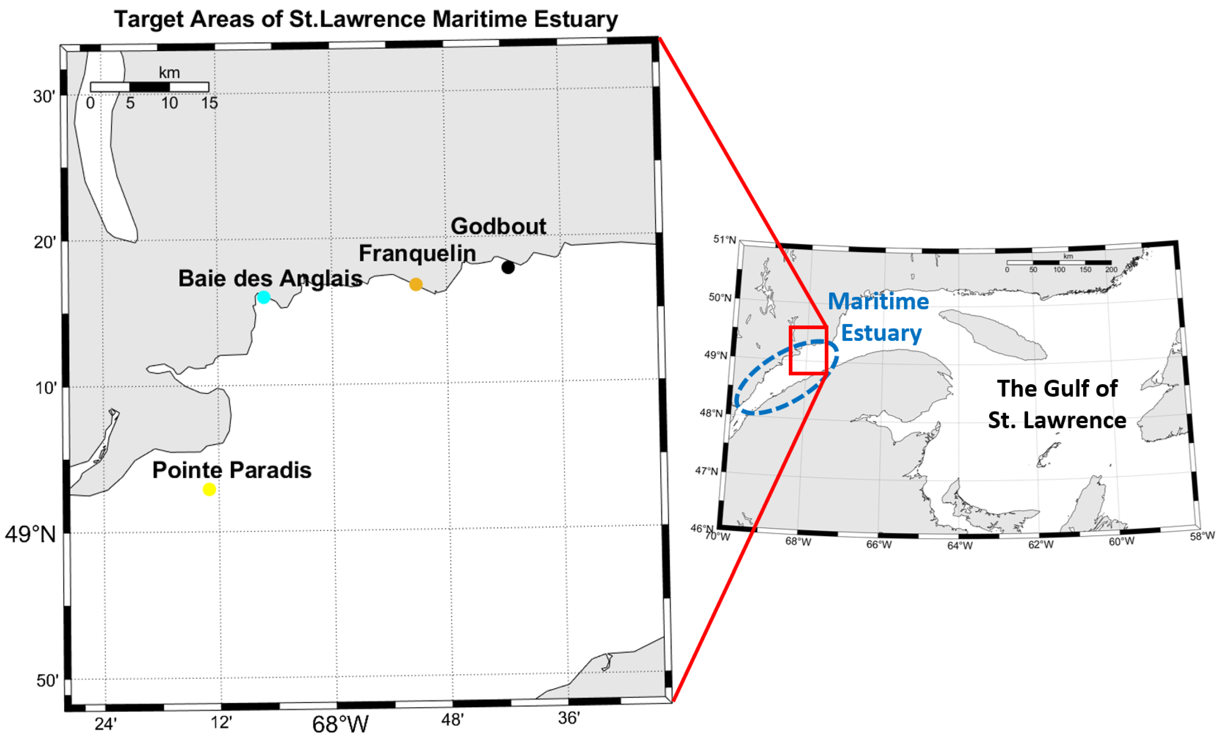
In the case of the surveys presented here, high-density MBES data have been gathered over several coastal regions of interest on the North Shore (
Figure 1). The study areas were surveyed using CIDCO’s hydrographic vessel, the FJ Saucier. The vessel’s hydrographic system is comprised of an IxBlue Hydrins inertial navigation system (INS), a Septentrio AsteRx-U GNSS, and a Reson SeaBat 7125 MBES. The system’s static calibration and offset measurements were conducted using a total station. The system’s dynamic calibration and boresight angles were measured using standard IHO patch-test methodology.
The positioning and attitude data were fused and corrected using real-time kinematics (RTK) and post-processed kinematics (PPK) whenever base station data were available. The bathymetry was computed using the CARIS HIPS and SIPS version 11.4 software suite. The raw bathymetry was smoothed using the CUBE algorithm [
19], and then decimated and interpolated to a 1 meter by 1 meter digital terrain model (DTM).
4.1.2. Ground-Truth Data
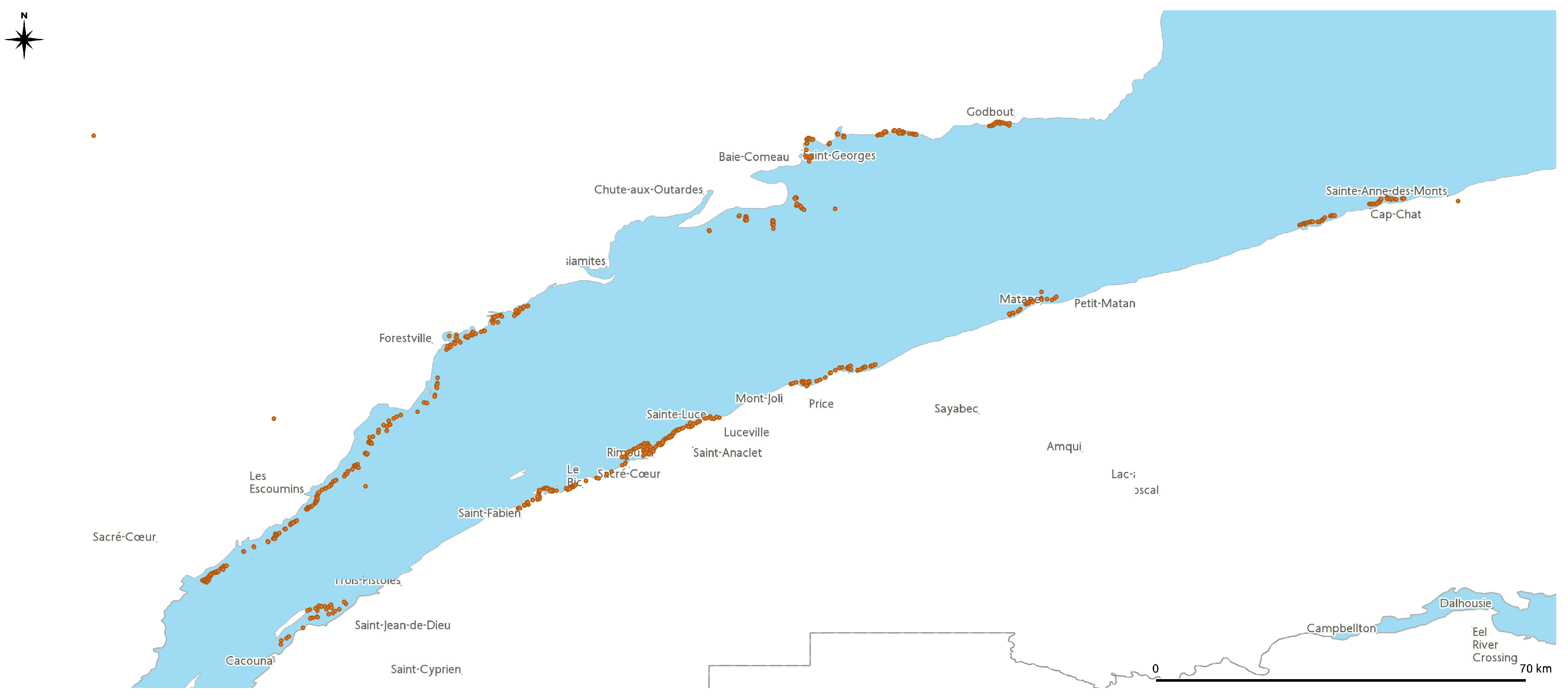
Fisheries and Oceans Canada (DFO) has developed a dictionary of underwater habitats, with data acquired at 905 coastal ground-truth stations (
Figure 2). The imagery at these stations has been acquired using drop camera setups, and the acquired images were interpreted by biologists to catalog substrate and vegetation variables for each location. Available for each station are longitude and latitude, the dominant three benthic substrates, and vegetation type if applicable. While the categorization could be optimized to improve precision by using a continuous variable for substrate size, we have decided to preserve the domain-specific class-oriented format that the employees of the Government of Canada are used to in order to generate directly transferable results.
4.1.3. Training Data Generation
In order to generate the training data, the 905 ground-truth stations’ data have been cross-referenced with the MBES data in order to obtain a neighborhood large enough to compute the feature vector for every ground station point. Ground-truth stations that did not fit the neighborhood requirements were discarded. Furthermore, to augment the data to consider multiple scales, soundings in a direct 3-meter neighborhood of the ground-truth stations were labeled with the class of their respective ground-truth station.
Habitat classes were derived from substrate particle size nomenclature provided by DFO in order to generate products meant to be helpful to biologists. Namely, we find bedrock, block, cobble, gravel, sand, and sandy mud classes.
4.2. Feature Engineering
The feature vector for each sounding is comprised of 16 geomorphometric variables (see
Table 1). These variables represent a geometric signature for each sounding that allows us to numerically describe a sounding and its neighborhood. This selection of 16 features were chosen for their solid establishment into the literature on applied geomorphometry to the hydroghraphic field [
16,
17]. Given a sounding
, we consider a neighborhood
N with
, on which we compute a local covariance matrix with eigenvalues
,
,
and their respective eigenvectors
,
,
:
This gives us a 16-dimensional feature vector to work with.
4.3. Supervised Learning
Several supervised learning algorithms have been tested as part of the comparative analysis, whose results can be found in
Table 2. The reference implementations were taken from the Scikit-Learn machine-learning library [
20]. This choice was made to leverage existing work with an established governance structure, an open-source implementation, and a mature technological stack.
4.3.1. K-Nearest Neighbors
First described by [
21], the K-nearest neighbors algorithm (KNN) is based on the idea that points that share a high amount of similarities in their features also share similarities in the classification variable. As such, we can use the Euclidean distance over the 16-dimensional feature vector to create a useful similarity metric, under the implicit assumption that a shorter distance between two points implies a higher similarity between them.
4.3.2. Support Vector Machines (SVM)
Introduced by [
22], the support vector machine has been a staple of both linear and non-linear classification problems due to its robustness. Anchored in the Vapnik–Chervonenkis statistical learning framework, the algorithm works on the principle of defining a boundary that maximizes the distance between categories by splitting the feature hyperspace using either hyperplanes in the linear case, or a kernel function in the non-linear case. Fresh data can then be categorized based on the class boundary.
4.3.3. Naive Bayes
The family of “naive” Bayes algorithms leverage Bayes’ theorem under the assumption of independence between the feature variables, hence the “naive” qualifier. While this independence is not always grounded in reality, this can often be used as a weak signal for classification. As such, this is more of an industry-standard reference figure than an optimal classifier but can still yield interesting performances, especially when considering how simple the method is.
4.3.4. AdaBoost
Adaptive boosting, or Adaboost, is an ensemble method advanced in [
23] that uses the output of several weak classifiers into a weighted sum to produce a strong classification. This meta-algorithm adapts the weights of each weak classifier’s output signal to improve the classification of misclassified points. For optimal performance, the Adaboost-SAMAA variant with decision trees as weak multiclass classifiers is used [
24].
4.3.5. Gradient Boosted Regression Trees
Gradient boosted regression trees is an ensemble method that uses successive approximations in order to generate a strong classification using a boosted set of weak decision tree classifiers. Building on the boosting theory of [
23], the idea of combining boosting and stochastic gradient descent methods was introduced in [
25] by using the residuals of each approximation step as the gradient of a loss-function to be minimized. Its claim to fame is that it generally performs better than random forests.
4.4. Unsupervised Learning
The fact that most of the world’s seafloor substrates have not been sampled reveals a definite lack of ground-truthing data for supervised methods. In this context, new methods that do not rely on ground-truthing data are necessary to fill the gap. To this end, we have devised an unsupervised method based on a Gaussian mixture models (GMM) based on the same feature space to blindly classify substrates. The core concept of GMM methods is to classify data under the assumption that they are made of a finite number of independent Gaussian distributions. The separation between distributions is carried out by estimating the center of each Gaussian and its associate covariance structure [
26]. In our case, we define the number of clusters as the number of substrates. To estimate the best fit in terms of cluster count, we use the Bayesian Information Criterion (BIC) [
27], whose efficiency is well established in the literature with parameter estimation successes reaching 90% [
28]. By finding the minimal BIC for an array of models, we thus find the best model fit for a given dataset. It is worth noticing that unlike supervised learning methods, this clustering is dependent on the underlying data and therefore does not generalize coherently to multiple independent datasets.
5. Results
By running models on each MBES dataset, we finally arrive at a fully classified dataset to generate habitat maps with GIS software. Here QGIS 3.22, a free and open-source GIS system, was used. The accuracy, precision, and recall of each supervised learning algorithm can be measured by using cross-validation with 20% of the dataset left out in the training phase to test out-of-bag soundings (
Table 2).
5.1. Model Performance
Supervised model performances (
Table 2) show that two algorithms stand out by their high accuracy rate, precision, and recall. The K nearest neighbors method comes in first with an accuracy of 91%, a precision of 90%, and a recall of 91%. Gradient boosted regression trees comes second with all three parameters to 91%. Since the gradient-boosted method gives the best performance, we shall use it from this point as the reference for supervised learning methods. Accuracy, precision and recall were computed as follows:
5.2. Comparative Analysis
Once trained, the supervised and unsupervised models have been applied on bathymetric datasets for a substrates classification in multiple areas of the North Shore of the St. Lawrence maritime estuary. Data created by the machine learning models are a sequence of positions (x,y,z) with an associated class with a numerical identifier. In both models, x,y, and z are the same values. In the case of the supervised model, the associated identifier is a number within the range of 0 to 5, respectively, corresponding to six different classes of substrates (block—0; cobble—1; gravel—2; bedrock—3; sand—4; and sandy mud—5). In the case of the unsupervised model, the identifier refers to distinct yet unknown classes, and the maximum number of different classes is determined by the number of clusters associated with the minimum BIC parameter. In order to qualitatively assess the comparison between the two methods, we analyze the correspondence between classes in each model.
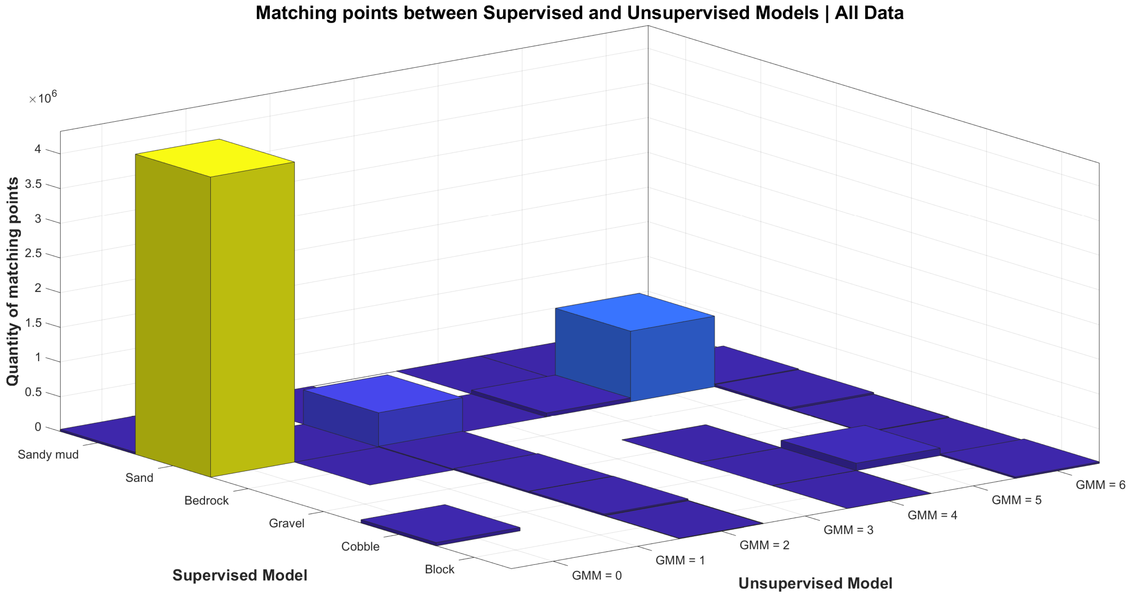
To this end, a simple algorithm has been devised: a matrix mapping the classes of the supervised model as rows and the classes of the unsupervised model as columns is set up (
Figure 3). The cell with the pair of supervised/unsupervised classes with the highest count is selected, and the rest of the cell’s row and column are set to 0. The process is repeated until all corresponding pairs are found. This yields the following correspondence matrix for our data, which confirms that the unsupervised method follows the human-like intuition that classes that are geometrically different, from a geomorphometric point of view, do correspond to different substrates.
5.3. Model-Generated Maps
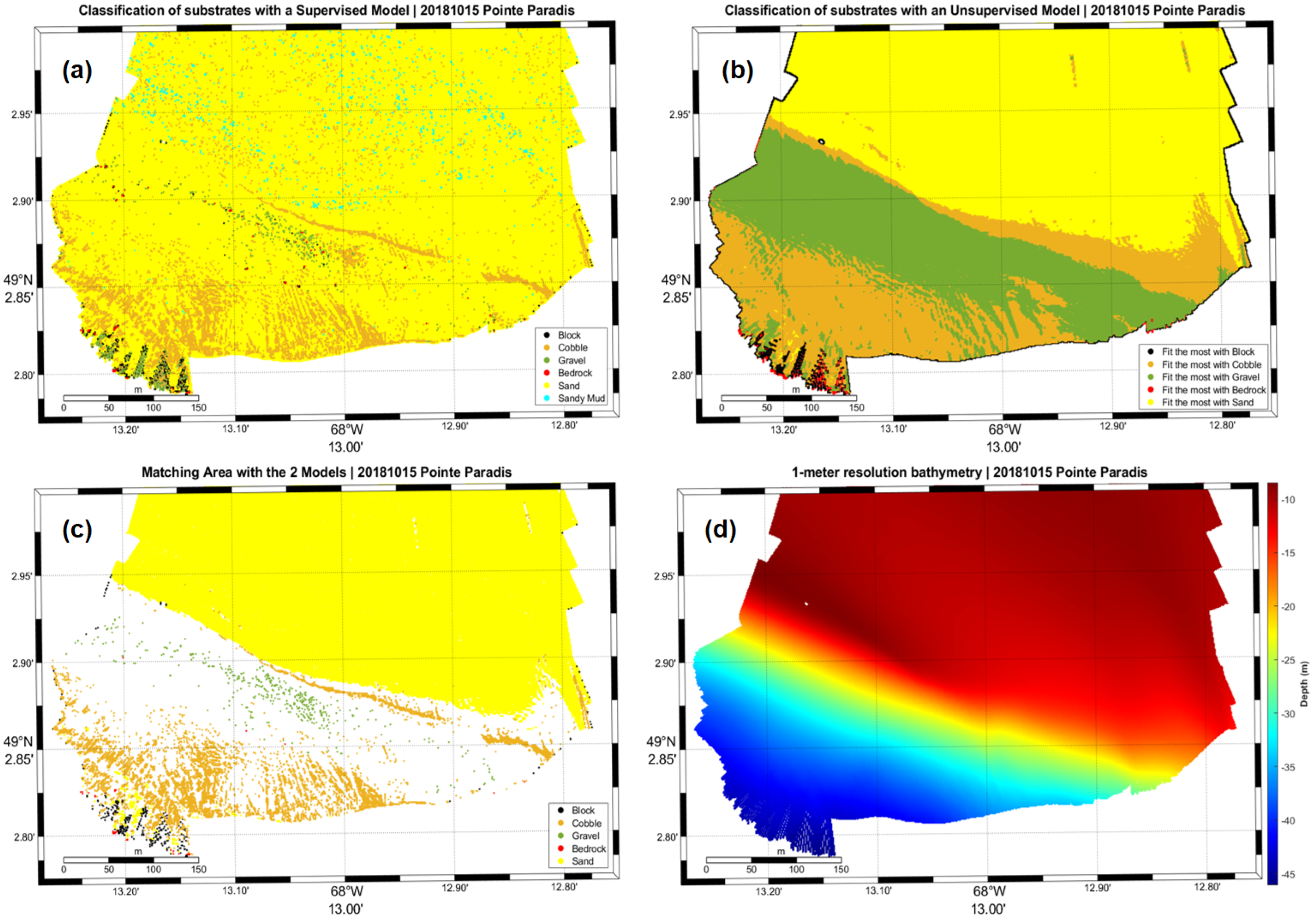
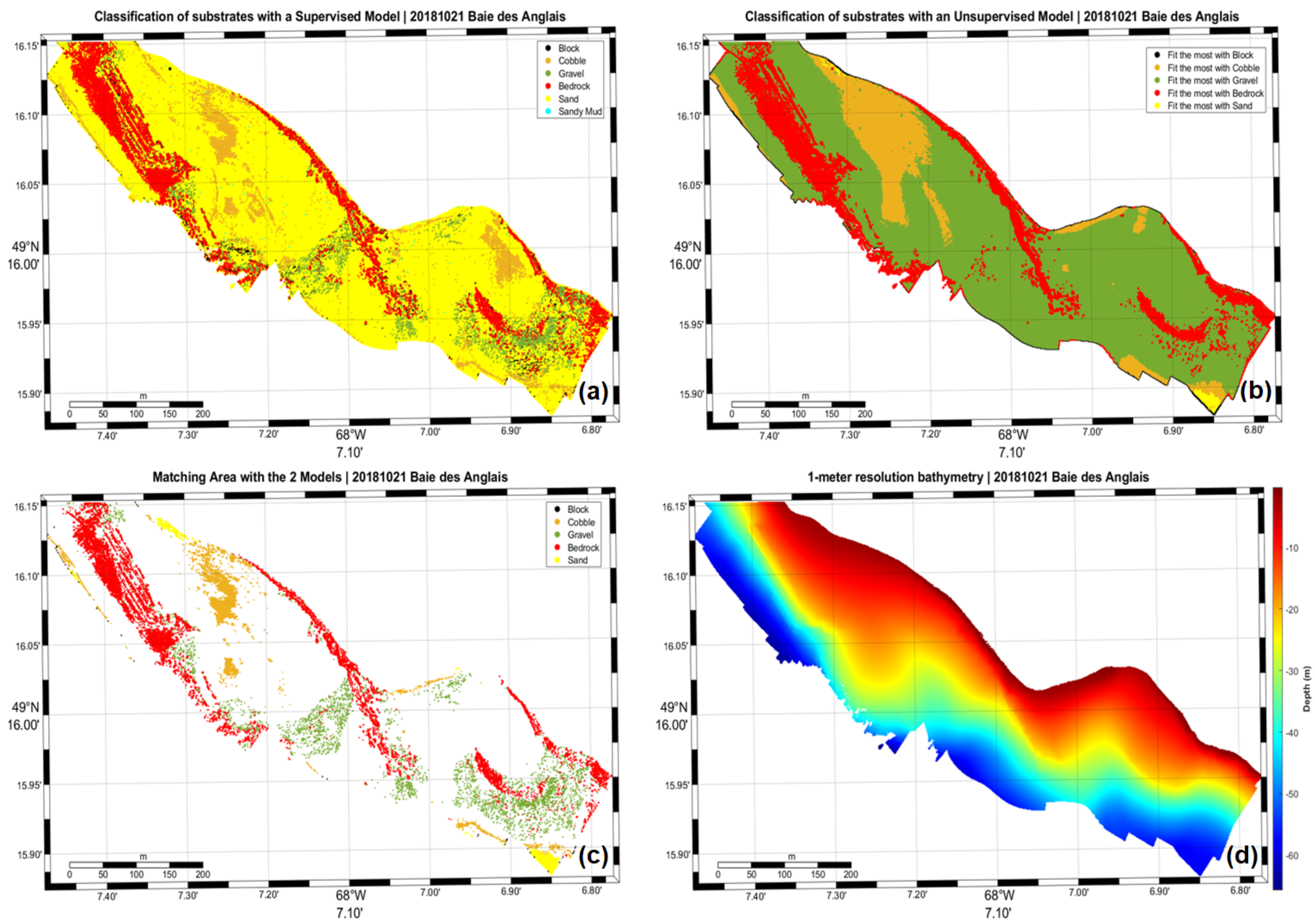
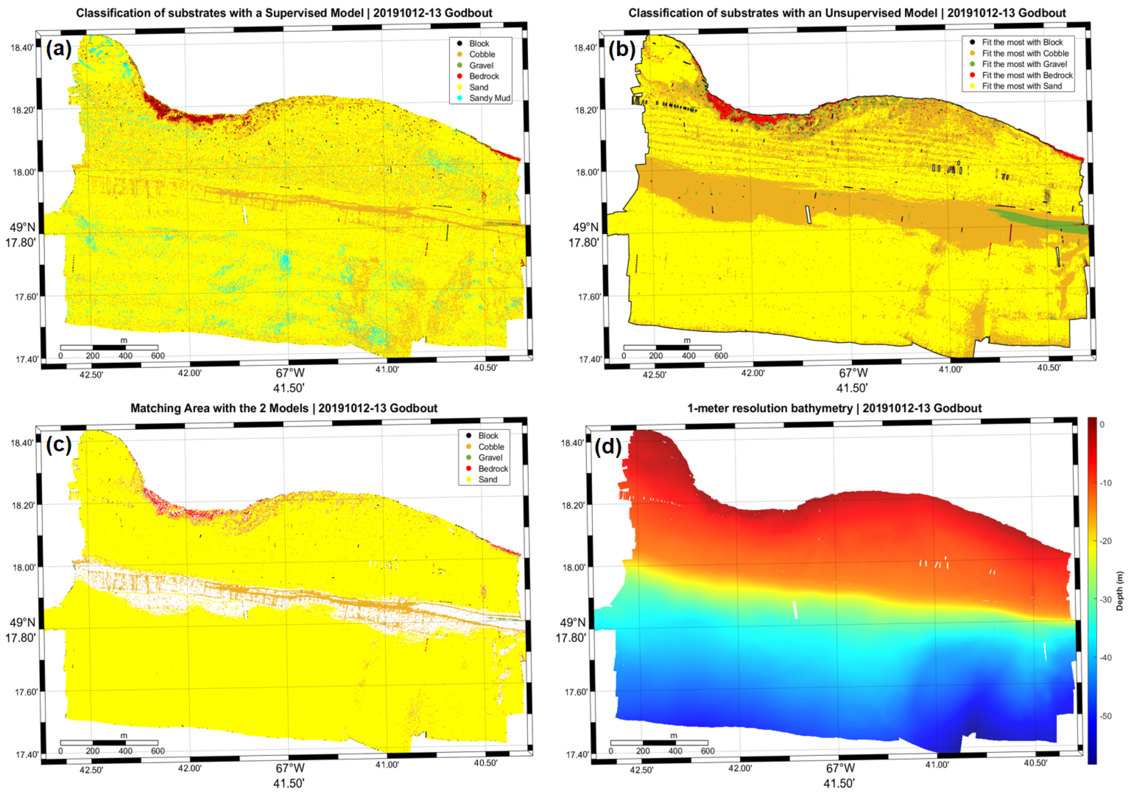
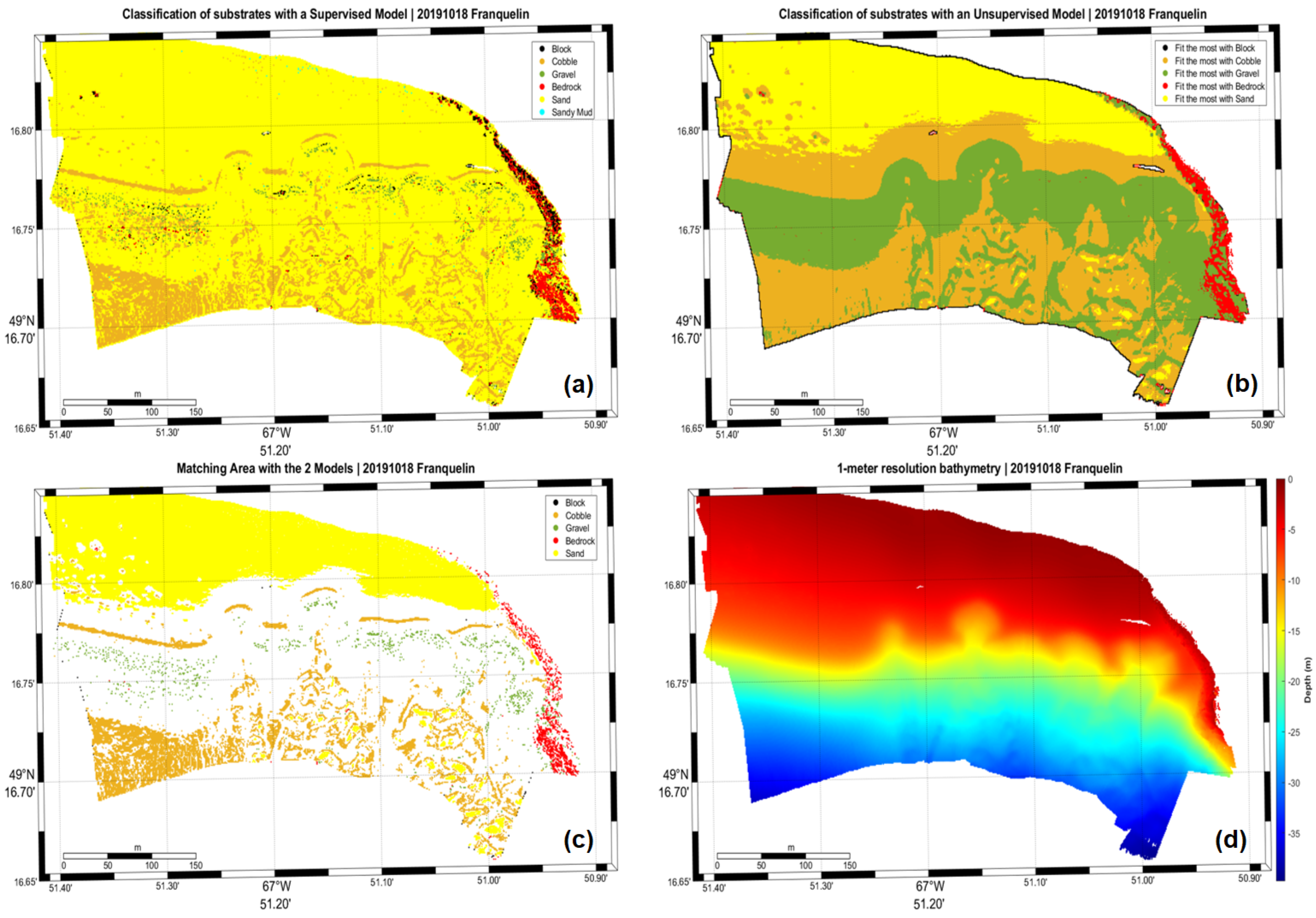
Maps shown in this section (
Figure 4,
Figure 5,
Figure 6 and
Figure 7) correspond to the supervised model data (a), the unsupervised model data (b), their matching area (c), and the 1-meter resolution bathymetry (d).
6. Discussion
Substrate classification using supervised learning and unsupervised learning on geomorphometric features derived from bathymetric data allows us to create detailed maps of the North Shore of the St. Lawrence Estuary.
The design choice of using solely geomorphometric variables can be argued. Several other proxy variables could be leveraged to enhance the model. Of particular interest is the strength of the acoustic return from the seafloor recorded by the echosounder (backscatter), which has been shown to be a very effective predictor [
29]. However, the acoustic strength is dependent on multiple environmental variables, and as such, lacks a common comparison basis. For example, the same seafloor may exhibit different acoustic return characteristics depending on the direction of surveying. Additionally, different sensors will yield different backscatter readings due to their inherent sensitivity differences. Research in the field of backscatter normalization should solve these issues in the future, but the current state of the art and the lack of availability of normalized backscatter datasets prevented it from being integrated into this research where a generalizable model was sought. Furthermore, relying solely on geomorphometric variables allows the method to be generalized to a large variety of remote sensing methods in addition to multibeam echosounders.
Supervised learning using gradient-boosting generates substrate classes based on ground-truth data (905 points distributed in all the maritime estuary). This model has a high performance based on its precision, accuracy, and recall (91%). On the other hand, even with the best performance, it is vulnerable to noise and artifacts, which can significantly alter the classification [
30]. We have encountered such an event as shown in
Figure 6 which is located in the Godbout area. Several artifacts emanating from calibration issues in the hydrographic system have confused the algorithm and led it to believe that a double line of cobbles was present instead of one at the 20-meter isobath. The proper equipment calibration is therefore critical before carrying out the hydrographic survey. The proper methodology must also be enforced to respect international standards with regard to hydrographic surveying best practices [
31].
Additionally, supervised learning is highly dependent on the classification system used by domain experts. This methodology depends heavily on the quality [
32] and quantity [
33] of substrate samples, which are assumed to have been perfectly collected and tagged by field operatives who will expertly interpret their classification. It also can be argued that the geometric signatures derived using coastal data may not generalize well to offshore study zones and that further research is warranted to validate the claim that these signatures would be free of such bias. This allows for the introduction of human error and bias in the training data, which strongly highlights the need for establishing proper governance and procedures around data acquired for the purpose of training artificial bits of intelligence, both of which come at a significant cost that adds on top of the considerable cost of acquiring field data for marine sciences.
Unsupervised learning classifications based on Gaussian mixture models [
26] do not require ground truthing data and can be applied to all areas where bathymetric data is available. It relies on an abstract geometrical distance definition, which has a nearly limitless range of possibilities in terms of model expansion to accommodate additional proxy variables. This flexibility and lack of a priori bias make it very suitable for exploratory analysis of the seafloor and anomaly detection. The Gaussian mixture model was chosen for ease of implementation and optimization through the minimum-BIC method. Further optimizations and model selection could be carried out as part of future research.
However, it follows from the arbitrary choice of substrate labels in the supervised learning model that not all classes have corresponding classes in each model, respectively. This is further exacerbated by the unsupervised model’s geometric distance definition based on geomorphometric features, which do not distinguish the differential characteristics of each feature with regard to its substrate classification, which results in some features weighing more in the unsupervised model’s perspective.
Furthermore, discrepancies between identical supervised classes referring to different unsupervised classes highlight the limitations of geomorphometric methods. Their dependence on geometric indicators can make them vulnerable to identical substrates forming different kinds of geometries, for example, sand formations that can be modeled into varied structures under the action of water currents, yielding different kinds of patterns such as dunes and such. This could be a promising area for further research.
Additionally, both models exhibit non-negligible edge effects at the extremities of the map, where the eigenvalues of the point’s neighborhood’s covariance matrix is either unstable of singular. This effectively results in the creations of singularities like in
Figure 4b,
Figure 5b,
Figure 6b and
Figure 7b.
Thus, the first results created with the unsupervised model are promising. Eventually, the current version of this model could be useful for flat sand-dominated areas and, to a lesser extent, for bedrock-dominated areas in an environmental study setting.
Another criticism of the method is the fact that both models are only trained on a 1-meter resolution bathymetry grid. Depending on the resolution of the seafloor required, both models could benefit from performing a multi-resolution analysis to adequately capture macroscopic phenomenons at different scales. This would effectively increase the number of parameters by multiplying the current parameter count by the number of different scales. These new models could be used to identify patterns that could not have been seen with a one-meter resolution dataset [
34].
7. Conclusions
The use of machine learning techniques to predict substrate classes based on geomorphometric features allows for promising habitat modeling processes. As such, the technique has proven itself to be very useful to efficiently map out benthic habitats and drastically reduce costs. As such, the techniques developed here can be leveraged as powerful automation mechanisms to open doors in improving resource monitoring in science, industry, and everywhere information on the characteristics of the seafloor is useful.
The use of a sparse DTM implies that the technique can be readily generalized to data coming from a large variety of sensors such as multibeam echosounders, aerial bathymetric lidar, satellite-derived bathymetry, and many more. Further research could easily leverage more than one remote sensing method to improve on this technique.
Author Contributions
Conceptualization, G.L.-M.; methodology, G.L.-M. and T.L.; software, G.L.-M., T.L., P.C.-M., D.G. and D.D.; validation, G.L.-M. and T.L.; formal analysis, G.L.-M., T.L., P.C.-M. and D.G.; investigation, G.L.-M., T.L., P.C.-M., D.G., D.D., M.-A.C. and D.N.M.; resources, D.D., M.-A.C. and D.N.M.; data curation, M.-A.C. and D.N.M.; writing—original draft preparation, G.L.-M. and T.L.; writing—review and editing, G.L.-M. and T.L.; visualization, T.L., P.C.-M. and D.G.; supervision, G.L.-M.; project administration, G.L.-M.; funding acquisition, G.L.-M. All authors have read and agreed to the published version of the manuscript.
Funding
This research was made possible with the support of the Department of Fisheries and Oceans from the Government of Canada under the Coastal Environmental Baseline Program.
Data Availability Statement
The raw data supporting the conclusions of this article will be made available by the authors on request.
Conflicts of Interest
The authors declare no conflicts of interest. The funders had no role in the design of the study; in the collection, analyses, or interpretation of data; in the writing of the manuscript; or in the decision to publish the results.
Abbreviations
The following abbreviations are used in this manuscript:
| BIC | Bayesian Information Criterion |
| DFO | Department of Fisheries and Oceans Canada |
| DTM | Digital Terrain Model |
| GBM | Gradient Boosting Method |
| GIS | Geographic Information System |
| GMM | Gaussian Mixture Method |
| GNSS | Global Navigation Satellite System |
| INS | Inertial Navigation System |
| MBES | Multibeam Echosounder |
| OECD | Organisation for Economic Co-operation and Development |
References
- NOAA. How Much of the Ocean Have We Explored? National Ocean Service Website; 2023. Available online: https://oceanexplorer.noaa.gov/facts/explored.html (accessed on 15 May 2023).
- Proudfoot, B.; Devillers, R.; Brown, C.J.; Edinger, E.; Copeland, A. Seafloor mapping to support conservation planning in an ecologically unique fjord in Newfoundland and Labrador, Canada. J. Coast. Conserv. 2020, 24, 36. [Google Scholar] [CrossRef]
- Flannagan, J.F. Efficiencies of Various Grabs and Corers in Sampling Freshwater Benthos. J. Fish. Res. Board Can. 1970, 27, 1691–1700. [Google Scholar] [CrossRef]
- Bouma, A. Methods for the Study of Sedimentary Structures; Wiley-Interscience: New York, NY, USA, 1969. [Google Scholar]
- Snellen, M.; Gaida, T.C.; Koop, L.; Alevizos, E.; Simons, D.G. Performance of multibeam echosounder backscatter-based classification for monitoring sediment distributions using multitemporal large-scale ocean data sets. IEEE J. Ocean. Eng. 2018, 44, 142–155. [Google Scholar] [CrossRef]
- Lurton, X.; Pouliquen, E. Automated Sea-bed Classification System For Echo-Sounders. In Proceedings of the OCEANS 92 Proceedings@m_Mastering the Oceans Through Technology, Newport, RI, USA, 26–29 October 1992; Volume 1, pp. 317–321. [Google Scholar]
- Pillay, T.; Cawthra, H.; Lombard, A. Characterisation of seafloor substrate using advanced processing of multibeam bathymetry, backscatter, and sidescan sonar in Table Bay, South Africa. Mar. Geol. 2020, 429, 106332. [Google Scholar] [CrossRef]
- Horning, N.; Robinson, J.A.; Sterling, E.J.; Turner, W. Remote Sensing for Ecology and Conservation: A Handbook of Techniques; Oxford University Press: Oxford, UK, 2010. [Google Scholar]
- Lyzenga, D.R.; Malinas, N.P.; Tanis, F.J. Multispectral bathymetry using a simple physically based algorithm. IEEE Trans. Geosci. Remote Sens. 2006, 44, 2251–2259. [Google Scholar] [CrossRef]
- Ma, S.; Tao, Z.; Yang, X.; Yu, Y.; Zhou, X.; Li, Z. Bathymetry Retrieval From Hyperspectral Remote Sensing Data in Optical-Shallow Water. IEEE Trans. Geosci. Remote Sens. 2014, 52, 1205–1212. [Google Scholar] [CrossRef]
- Haralick, R.M.; Shanmugam, K.; Dinstein, I.H. Textural features for image classification. IEEE Trans. Syst. Man Cybern. 1973, SMC-3, 610–621. [Google Scholar] [CrossRef]
- Geisz, J.K.; Wernette, P.A.; Esselman, P.C. Classification of Lakebed Geologic Substrate in Autonomously Collected Benthic Imagery Using Machine Learning. Remote Sens. 2024, 16, 1264. [Google Scholar] [CrossRef]
- Wahidin, N.; Siregar, V.P.; Nababan, B.; Jaya, I.; Wouthuyzen, S. Object-based Image Analysis for Coral Reef Benthic Habitat Mapping with Several Classification Algorithms. Procedia Environ. Sci. 2015, 24, 222–227. [Google Scholar] [CrossRef]
- Jackett, C.; Althaus, F.; Maguire, K.; Farazi, M.; Scoulding, B.; Untiedt, C.; Ryan, T.; Shanks, P.; Brodie, P.; Williams, A. A benthic substrate classification method for seabed images using deep learning: Application to management of deep-sea coral reefs. J. Appl. Ecol. 2023, 60, 1254–1273. [Google Scholar] [CrossRef]
- Arosio, R.; Hobley, B.; Wheeler, A.J.; Sacchetti, F.; Conti, L.A.; Furey, T.; Lim, A. Fully convolutional neural networks applied to large-scale marine morphology mapping. Front. Mar. Sci. 2023, 10, 1228867. [Google Scholar] [CrossRef]
- Hackel, T.; Wegner, J.D.; Schindler, K. Fast Semantic Segmentation of 3D Point Clouds With Strongly Varying Density. ISPRS Ann. Photogramm. Remote Sens. Spat. Inf. Sci. 2016, 3, 177–184. [Google Scholar] [CrossRef]
- Lecours, V.; Dolan, M.F.; Micallef, A.; Lucieer, V.L. A review of marine geomorphometry, the quantitative study of the seafloor. Hydrol. Earth Syst. Sci. 2016, 20, 3207–3244. [Google Scholar] [CrossRef]
- Misiuk, B.; Brown, C.J. Benthic habitat mapping: A review of three decades of mapping biological patterns on the seafloor. Estuar. Coast. Shelf Sci. 2023, 296, 108599. [Google Scholar] [CrossRef]
- Calder, B. Automatic Statistical Processing of Multibeam Echosounder Data. Int. Hydrogr. Rev. 2003, 4, 53–68. [Google Scholar]
- Pedregosa, F.; Varoquaux, G.; Gramfort, A.; Michel, V.; Thirion, B.; Grisel, O.; Blondel, M.; Prettenhofer, P.; Weiss, R.; Dubourg, V.; et al. Scikit-learn: Machine Learning in Python. J. Mach. Learn. Res. 2011, 12, 2825–2830. [Google Scholar]
- Fix, E.; Hodges, J.L. Discriminatory Analysis. Nonparametric Discrimination: Consistency Properties. Int. Stat. Rev./Rev. Int. De Stat. 1989, 57, 238–247. [Google Scholar] [CrossRef]
- Boser, B.E.; Guyon, I.M.; Vapnik, V.N. A training algorithm for optimal margin classifiers. In COLT ’92: Proceedings of the Fifth Annual Workshop on Computational Learning Theory, Pittsburgh, PA, USA, 27–29 July 1992; ACM Press: New York, NY, USA, 1992; pp. 144–152. [Google Scholar]
- Freund, Y.; Schapire, R.E. A Short Introduction to Boosting. In Proceedings of the Sixteenth International Joint Conference on Artificial Intelligence, Stockholm, Sweden, 31 July–6 August 1999; Morgan Kaufmann: Burlington, MA, USA, 1999; pp. 1401–1406. [Google Scholar]
- Hastie, T.; Rosset, S.; Zhu, J.; Zou, H. Multi-class AdaBoost. Stat. Its Interface 2009, 2, 349–360. [Google Scholar] [CrossRef]
- Friedman, J.H. Stochastic Gradient Boosting. Comput. Stat. Data Anal. 2002, 38, 367–378. [Google Scholar] [CrossRef]
- Reynolds, D.A. Gaussian mixture models. Encycl. Biom. 2009, 741, 659–663. [Google Scholar]
- Schwarz, G. Estimating the dimension of a model. Ann. Stat. 1978, 461–464. [Google Scholar] [CrossRef]
- Steele, R.; Raftery, A.E. Performance of Bayesian model selection criteria for Gaussian mixture models. Front. Stat. Decis. Mak. Bayesian Anal. 2010, 2, 113–130. [Google Scholar]
- Brown, C.J.; Beaudoin, J.; Brissette, M.; Gazzola, V. Multispectral Multibeam Echo Sounder Backscatter as a Tool for Improved Seafloor Characterization. Geosciences 2019, 9, 126. [Google Scholar] [CrossRef]
- Gupta, S.; Gupta, A. Dealing with noise problem in machine learning data-sets: A systematic review. Procedia Comput. Sci. 2019, 161, 466–474. [Google Scholar] [CrossRef]
- Mills, G.B. International hydrographic survey standards. Int. Hydrogr. Rev. 1998. [Google Scholar] [CrossRef]
- Long, D. BGS Detailed Explanation of Seabed Sediment Modified Folk Classification. MESH (Mapping European Seabed Habitats); 2006. Available online: https://webarchive.nationalarchives.gov.uk/ukgwa/20101014090013/http://www.searchmesh.net/PDF/GMHM3_Detailed_explanation_of_seabed_sediment_classification.pdf (accessed on 15 May 2023).
- Weiss, G.M.; Provost, F. Learning when training data are costly: The effect of class distribution on tree induction. J. Artif. Intell. Res. 2003, 19, 315–354. [Google Scholar] [CrossRef]
- Blayvas, I.; Kimmel, R. Machine learning via multiresolution approximation. Ieice Trans. Inf. Syst. 2003, 86, 1172–1180. [Google Scholar]
| Disclaimer/Publisher’s Note: The statements, opinions and data contained in all publications are solely those of the individual author(s) and contributor(s) and not of MDPI and/or the editor(s). MDPI and/or the editor(s) disclaim responsibility for any injury to people or property resulting from any ideas, methods, instructions or products referred to in the content. |
© 2024 by the authors. Licensee MDPI, Basel, Switzerland. This article is an open access article distributed under the terms and conditions of the Creative Commons Attribution (CC BY) license (https://creativecommons.org/licenses/by/4.0/).
