Mapping and Geomorphic Characterization of the Vast Cold-Water Coral Mounds of the Blake Plateau

Abstract

A coordinated multi-year ocean exploration campaign on the Blake Plateau offshore of the southeastern U.S. has mapped what appears to be the most expansive cold-water coral (CWC) mound province thus far discovered. Nearly continuous CWC mound features span an area up to 500 km long and 110 km wide, with a core area of high-density mounds up to 254 km long by 42 km wide. This study synthesized bathymetric data from 31 multibeam sonar mapping surveys and generated a standardized geomorphic classification of the region in order to delineate and quantify CWC mound habitats and compare mound morphologies among subregions of the coral province. Based on the multibeam bathymetry, a total of 83,908 individual peak features were delineated, providing the first estimate of the overall number of potential CWC mounds mapped in the region to date. Five geomorphic landform classes were mapped and quantified: peaks (411 km²), valleys (3598 km²), ridges (3642 km²), slopes (23,082 km²), and flats (102,848 km²). The complex geomorphology of eight subregions was described qualitatively with geomorphic “fingerprints” (spatial patterns) and quantitatively by measurements of mound density and vertical relief. This study demonstrated the value of applying an objective automated terrain segmentation and classification approach to geomorphic characterization of a highly complex CWC mound province. Manual delineation of these features in a consistent repeatable way with a comparable level of detail would not have been possible.

1. Introduction

Cold-water corals (CWCs) grow in the absence of sunlight in deeper water of the world’s oceans and filter feed on suspended particles in the water column [1]. CWCs have been documented to inhabit many parts of the deep ocean once thought to support minimal benthic fauna. The global distribution of CWC species remains poorly understood given that the majority of the global deep ocean is yet to be mapped or explored [2]. However, CWCs appear to be mainly restricted to oceanic waters within a temperature range of 4–14 °C that are well oxygenated and saturated in the relevant forms of calcium carbonate [1,3,4]. Many CWC species are affiliated with hard substrates and geologic features that offer steeper slopes, exposed bedrock, or coarse drop-stone materials for attachment to the seafloor [5,6,7]. Dense aggregations of CWCs are also associated with regions of the ocean that sustain high primary productivity in overlying waters and reliable currents for food delivery to the stationary corals [5,8].

Some CWC species can build calcium carbonate-based reef structures referred to by a variety of terms including coral banks, lithoherms, and bioherms [9,10,11]. A bioherm is a type of mound composed of unconsolidated sediment and coral skeletal material capped with coral thickets [10], whereas a lithoherm is a mound composed of high-relief lithified carbonate that may be covered with live coral [12]. CWC reefs have been documented off the coasts of at least 41 countries thus far [13], and recent global models predict an even wider distribution [14].

Cold-water scleractinian (“stony coral”) taxa such as Desmophyllum pertusum (previously named Lophelia pertusa), Enallopsammia, Madrepora, Oculina, and Solenosmilia grow dense calcareous skeletal frameworks that can build extensive biogenic coral mounds ranging in vertical relief from tens to hundreds of meters [15]. These mound features have been discovered around the world clustering in “provinces” where food supply and strong currents support coral growth [16]. These CWC reefs provide complex structure and hard substrate that provide habitat for many associated corals, sponges, invertebrates, and fishes [17,18,19]. Reef-forming CWC species therefore serve as autogenic “ecosystem engineers” (also referred to as foundation species) by substantially modifying the surrounding environment and creating habitat niches for many other species [20]. There is also evidence that the presence of high-relief CWC mounds can affect the overlying physical oceanography. For example, CWC mounds at 600 m depth on Rockall Bank in the NE Atlantic have been shown to induce tidally driven downwelling of organic material, providing an important carbon pump from surface waters to the deep sea [21].

CWC habitats are slow-growing, long-lived, and fragile, making them particularly vulnerable to physical damage from human activities that disturb the seafloor. Threats include trawling [22], hydrocarbon and mineral exploration and production [23], and cable and pipeline placements [13]. The ecological importance and vulnerability of CWC reefs has resulted in increased national and international efforts to map, characterize, and protect them [24].

Multibeam sonar systems have enabled ocean scientists to map complex CWC mound and reef habitats remotely from surface ship hull-mounted sonars (example shown in Figure 1 for the Richardson Mounds subregion of this study). The resolution of these seafloor maps is directly related to the depth of the seafloor and the angular resolution of the particular multibeam system, but it should be possible to resolve mound features using this tool to a depth of approximately 1500 m depending on the sonar, surveying conditions and speed, and size of the mound features. Multibeam and sidescan sonar systems mounted on remotely operated vehicles (ROVs) and autonomous underwater vehicles (AUVs) can reach close to the seafloor and thereby obtain much higher resolution maps of CWC mounds—typically centimeters to tens of meters resolution depending on the height above the seafloor [25,26]. These systems provide higher resolution but smaller areas of coverage than ship-mounted multibeam sonars. Fine-scale ground-truth data on seafloor substrate character and biological communities at CWC sites is made possible through the use of towed or dropped camera systems, and via video data collected by AUVs, ROVs, and human occupied vehicles (HOVs) that can capture views of these habitats within meters of the seafloor.

Aggregations of CWC mounds are regularly referred to in the scientific literature as “provinces” [27,28,29,30]. While there is no clear standard that defines a province, by convention they describe groups of CWC mounds that often span tens of square kilometers. The delineation of CWC provinces is pragmatically useful for management and conservation purposes such as designation of seafloor areas where bottom-disturbing activities are prohibited [27].

The region offshore of the southeastern U.S. contains the most extensive Desmophyllum pertusum (previously referenced in the literature as Lophelia pertusa) and Oculina CWC ecosystems documented within U.S. waters [11,31,32,33,34,35]. Desmophyllum pertusum is the most common reef-building CWC documented in the North Atlantic and has been found in depths ranging from 39 to 3383 m [13,36], but it is most commonly found between about 200 about 1000 m. Studies in the Gulf of Mexico on artificial structures calculated minimum Desmophyllum pertusum growth rates of 3.2 to 32.3 mm/year [37]. CWC mounds within the Straits of Florida have displayed growth throughout changes in geologic climate cycles over the last 600,000 years, including the last glacial maximum [38]. Given the slow growth rates of Desmophyllum pertusum, and that dead coral samples from mound features on the Blake Plateau have thus far been dated between 5000 and 44,000 years old [39], the size and nature of the mounds features in the Blake Plateau indicate that they must be many thousands of years old and would be very slow to recover from physical damage from human activities.

In response to improved information on the nature and distribution of CWC resources on the Blake Plateau, the South Atlantic Fishery Management Council (SAFMC) designated the Stetson/Miami Terrace Deep Water Coral Habitat Area of Particular Concern (HAPC) in 2010 to protect the seafloor in this area. The designation prohibits the use of bottom-contact fishing gear (bottom longline, bottom and mid-water trawl, dredge, pot, and trap), anchoring by fishing vessels, and possession of deep-water coral [40].

In 2016, the National Oceanic and Atmospheric Administration’s (NOAA) Deep Sea Coral Research and Technology Program initiated the Southeast Deep Coral Initiative (SEDCI)—a focused four-year research effort to dramatically increase exploration and understanding of deep-sea coral habitats in the southeastern region of the U.S. [41]. The science plan for this initiative informed much of the exploration work and data partially synthesized and presented in this study. In conjunction with SEDCI and under the auspices of the Atlantic Seafloor Partnership for Integrated Research and Exploration (ASPIRE), NOAA Ocean Exploration and partners conducted 16 expeditions focused on collecting new mapping and imagery data to close large gaps throughout the southeast region. A separate but related key research initiative in the southeastern U.S. region was launched in 2017 called Deep-Sea Exploration to Advance Research on Corals/Canyons/Cold seeps (DEEP SEARCH) with funding from the National Oceanographic Partnership Program [42]. New mapping data and submersible video data from DEEP SEARCH were utilized in this study for pertinent regions of the Blake Plateau.

The strategic ocean exploration efforts led by NOAA Ocean Exploration and the DEEP SEARCH project provided breakthrough insights into the nature and extent of the CWC ecosystems of the Blake Plateau off the southeastern United States. This study used data collected by these initiatives, along with other publicly available mapping surveys, to compile mapping data and video annotations interpreted from submersible human-occupied vehicle (HOV) and remotely operated vehicle (ROV) video footage to achieve the following:

• Determine the known extent of CWC mound features;
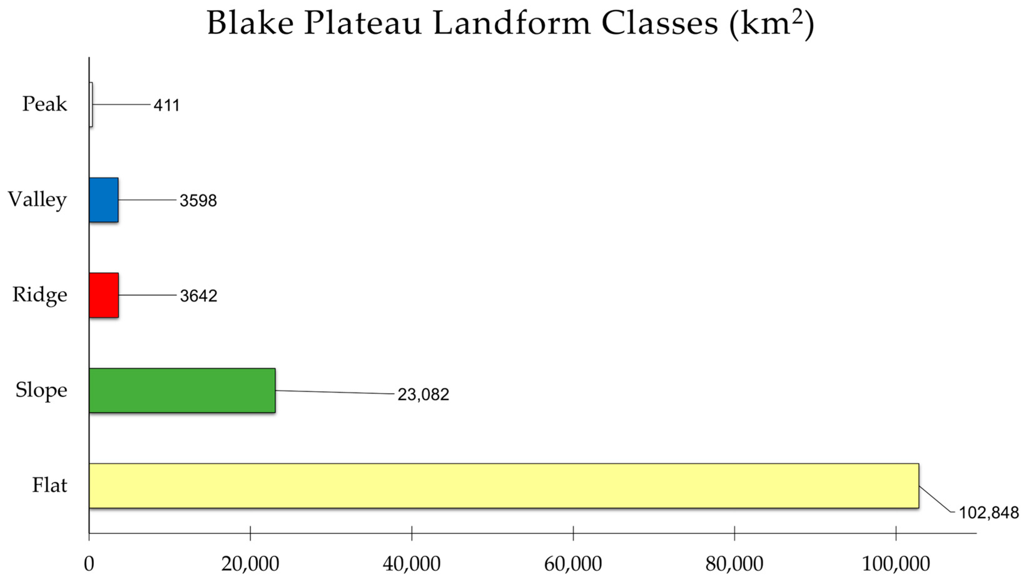
• Generate an objective standardized geomorphic characterization of the region;
• Examine the relationship between mound landforms and seafloor substrates;
• Test the application of the Coastal and Marine Ecological Classification Standard (CMECS) to substrates and geomorphic features in the study area [43].

This study presents a synthesis of all high quality multibeam sonar bathymetry from the Blake Plateau to produce a nearly complete coverage map. It then uses this synthesis to identify, classify, and characterize potential CWC habitats to inform management and conservation efforts in the region. Innovative aspects of this study include the application of a standardized repeatable methodology for geomorphic terrain analysis of a CWC province, presenting an effective approach to enumerating the large number of potential CWC mounds in a region, and generating descriptive metrics of CWC mound vertical relief relative to the surrounding seafloor terrain.

2. Materials and Methods

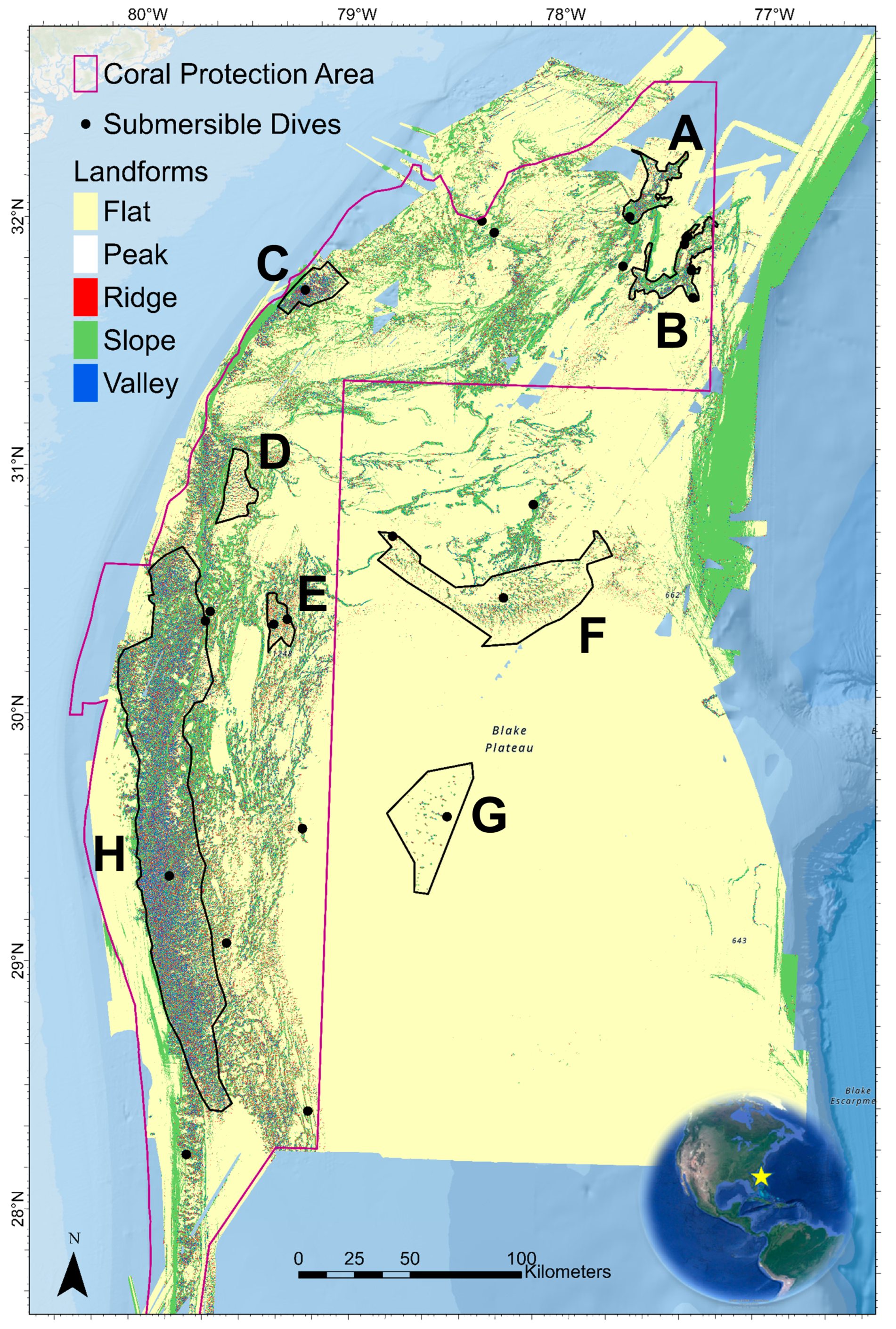
2.1. Study Area

The study area is located on the Blake Plateau 60–120 km offshore of the southeast U.S. coastline beginning roughly southeast of Miami, Florida, in the south (~25° N) and ending southeast of Charleston, South Carolina, in the north (~32.4° N). The Blake Plateau is a broad, relatively flat region of the U.S. Atlantic continental margin ranging from about 500 to 1000 m water depth (refer to Figure 2). The 150–300 km wide plateau is located between the shallow continental shelf (<200 m depth) and the Blake Escarpment continental slope that steeply drops to abyssal plains at 5000 m. The study area is 133,581 km² (almost the size of the state of Florida) and includes the western region of the Blake Plateau that is directly influenced by the main axis of the warm Florida Current/Gulf Stream current as it moves northward out of the Straits of Florida. The current extends to the seafloor in this area with a mean transport of 32 Sverdrup (Sv, one million cubic meters per second) at 27° N (±2–3 Sv for seasonal and interannual variability), which is equivalent to about two thousand times the annual average transport of the Mississippi River into the Gulf of Mexico [44,45]. Gulf Stream transport varies seasonally, with surface water transport peaking in the fall and reaching a minimum in the spring but deep-water transport showing the opposite seasonal peak fluctuations and with a larger magnitude [46]. The study area encompasses subregions of the Blake Plateau referred to by other researchers under a variety of names, including Stetson Reefs [10], Stetson Banks [35], Savannah Banks [47], Hoyt Hills, Richardson Hills, Richardson Reef [31], “Million Mounds,” and portions of the Miami Terrace and Charleston Bump.

2.2. Bathymetric Synthesis and Estimation of the Largest CWC Province on the Blake Plateau

Data from 31 separate multibeam sonar mapping surveys completed between 2003 and 2021 were synthesized into a seamless bathymetric terrain model with 35 m grid resolution. This grid resolution was the finest possible that could accommodate all of the data sources for the study area. The largest areas were covered by seventeen expeditions led by the NOAA Ocean Exploration on the NOAA Ship Okeanos Explorer, five mapping surveys completed by the NOAA Ship Nancy Foster, two expeditions led by the DEEP SEARCH project on the NOAA Ship Ronald H. Brown and R/V Atlantis, and one mapping survey Fugro vessel Brasilis completed for NOAA Ocean Exploration. Bathymetric data, as well as submersible dive video data, were utilized from all of these cruises to inform this study. Bathymetric data processing is described in this section, while utilization of dive video data is described in Section 2.5.

All data used as input to the bathymetric grid are publicly available via the NOAA National Centers for Environmental Information multibeam archives. Data incorporated into the grid are from the following cruises: EX1106, EX1202L1, EX1203, EX1403, EX1804, EX1805, EX1806, EX1812, EX1903L1, EX1903L2, EX1906, EX1907, EX2101, EX2102, EX2105, EX2106, EX2107, KR-OER-1901, RB1903, AT41, H11071, H11680, LCE2010, RB1008, SAB2006, NF0702, NF0913, NF2106, NF2107, H13528, and PAT0503. Bathymetric data spanned a range of 59–2717 m, with a mean depth of 813 m. These data cover the vast majority of the Blake Plateau, with only a few small gaps left to be mapped with modern multibeam sonar. Multibeam sonar lines from any survey with poor quality (typically resulting from rough weather conditions) were not used.

Data from each survey were quality checked and rigorously cleaned of noise and sound speed error artifacts using manual and automated editing tools within QPS Qimera software version 2.2.3. Most of the data were collected by a Kongsberg EM 302 multibeam sonar on the Okeanos Explorer with a 0.5° × 1° transmit/receive beam width array that supported consistent quality 25 m resolution grids of the study region. Cleaned data from all sources were gridded to 25 to 35 m resolution depending on the source data quality. These individual survey grids were then exported in xyz (longitude, latitude, depth) format, reimported into a master synthesis Qimera project, and then incorporated into a seamless 35 m resolution dynamic surface. Gridding surfaces were created using Qimera’s weighted moving average algorithm with a 3 × 3 cell moving window. Some minor artifacts were present in the far northern portion of the synthesis grid in areas where different surveys overlapped.

This region of the Blake Plateau has extremely dynamic sound speed fluctuations in the water column due to the Gulf Stream and associated eddies, but most artifacts resulting from sound speed error were resolved through editing of outer beams of the sonar swaths in the Qimera software. This intensive quality control editing of the synthesis bathymetric grid was completed in order to produce the best possible seamless map of the region so as to minimize artifacts that would affect the results of geomorphic classification in the next step of the study (Section 2.3). The bathymetry grid and all other spatial datasets used in the study were projected to spatial reference WGS 84/UTM zone 18N (EPSG:32618). The final 35 m resolution bathymetry grid was imported into ArcGIS Pro version 3.1.0. for further analysis.

The seamless bathymetry grid (Figure 2) was used to delineate the extent of nearly continuous CWC mound and scarp areas in the south and west portion of the study region that encompasses the largest area and densest mound features as the largest CWC mound “province” on the Blake Plateau. Mound-shaped features with a minimum of 3–4 m vertical relief from the surrounding seafloor are discernible in the bathymetric grid, and they were considered potential CWC mounds for this study. Since there is not an agreed upon standard for what defines a CWC mound province, two different regions were delineated to approximate a maximum and minimum extent in order to enable comparison with the areal coverage of other CWC mound provinces globally. Determining “nearly continuous” in terms of CWC mounds is a subjective process since many mound features in proximity to each other do not directly touch. For this reason, two different polygons were manually drawn in ArcGIS Pro using different criteria. The maximum extent polygon (black dashed line polygon in Figure 2) was drawn liberally to include any areas of adjacent scarp and CWC mound features with the outer boundary being digitized where all features ceased and only flat seafloor was evident in the multibeam grid. This maximum extent polygon therefore includes some areas of large flats that are surrounded by mound and scarp features, areas with very small mound features (down to 3 m vertical relief), and some areas of low mound densities. The approximate location and names of some of the previously documented study sites on the Blake Plateau are shown as black point features in Figure 2 in order to provide context in relation to this study.

A second smaller polygon was digitized to only include the core area of very dense mound aggregations within the maximum extent polygon. The purpose of this polygon was to define an extent of nearly continuous CWC mound features that is very conservative and essentially limited to places where the base of one mound slope touches an adjacent mound (white polygon in Figure 2). There is a fairly distinct landscape morphology change moving from west to east within this area: from densely packed mounds to more widely spaced mounds in the southern half, and a shift to scarp and ridge features in the northern half. The approximate transition between these different east/west morphologies was used to define the eastern edge of the core area polygon. The Kernel Density tool in ArcGIS Pro was also run on terrain features classified as peaks, and the area where peak kernel density transitioned from a value of 4 to 3 was used as a less subjective aid to help digitize the core area boundary. The core area of dense mounds is referred to in this study as the “Million Mounds” subregion based on a nickname it was given by scientists during mapping and ROV expeditions to convey the excitement of revealing the full extent of such a large CWC ecosystem. As revealed by this study, the nickname is in fact a misnomer given that this subregion actually appears to contain 35,789 possible CWC mounds.

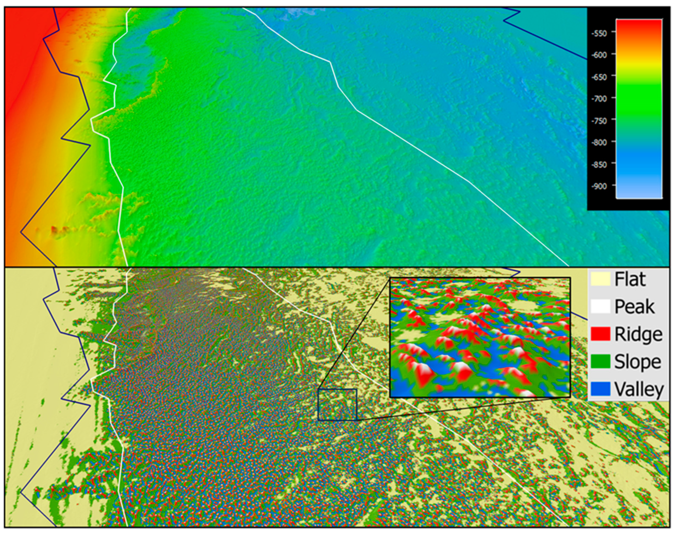
2.3. Objective Geomorphic Analysis of the Study Area

Beyond mapping the plateau and identifying the largest continuous areas of CWC mound distribution, this study applied a repeatable and objective approach to characterizing the geomorphology at the scale of individual mound features as well as the region as a whole. An objective geomorphic landform classification of the region was derived from the bathymetry using the bathymetry- and reflectivity-based estimator for seafloor segmentation (BRESS) method [48]. The geomorphic classification approach taken in this study builds on methods applied to the Atlantic continental slope, abyssal plains, and seamounts along the U.S. Atlantic margin [49,50], and the reader is referred to these publications for discussion of selecting and testing suitable modeling parameters for a given study area. Dolan and Bjarnadóttir [51] utilized a similar application of BRESS to complete a morphometric features classification in the Barents and Norwegian Seas, Norway. Details about the theoretical framework of this approach can be found in the 2013 study by Jasiewicz and Stepinski [52]. BRESS is available as a free stand-alone application at https://www.hydroffice.org/bress/main (accessed on 2 November 2023) [53]. Version 2.4.0 was utilized for this study.

The BRESS analytical approach identifies terrain features that can be classified into easily recognizable landform types such as valleys, slopes, ridges, and flats. These landform archetypes are referred to as “bathymorphons” and represent the relative landscape relationships between a single node in the bathymetric grid and the surrounding grid nodes as assessed in eight directions around the node. This relative position is determined via a line-of-sight method looking out in each direction by a user-defined search annulus specified by an inner and outer search radius. The algorithm generates aggregations of the same bathymorphon type and utilizes a look-up classification table to translate these patterns into landform types.

The bathymetric terrain analysis approach used in BRESS differs in some distinct aspects with the widely used bathymetric position index (BPI) calculated using ESRI’s Benthic Terrain Modeler tool [54]. BPI analysis generates numeric values for each cell based on the depth difference between the cell and the mean of all other cells within a surrounding search annulus. BPI is typically computed at two scales—broad and fine scale. The user then decides what range of BPI values should be used in a classification table, along with other user-determined variables, to classify marine habitats of interest. The BRESS approach was used in this study because the purpose was to generate a single unified classification of geomorphic features—in contrast to generating a suite of terrain variables for input into a benthic habitat classification study.

The classification types for this study were selected to delineate the most essential components of CWC mound and geologic scarp features that comprise the notable geomorphic features in the study region, while striving for simplicity. A driving determinant of the selection of landform classes was to effectively delineate and quantify CWC mound peak features from the rest of the terrain. This objective was critical as assessing the number, density, and vertical relief of CWC mound features across the extent of the region and comparing among subregions was deemed an essential way to characterize the CWC province. The following landform types were selected to meet the study goals while enabling the classification of a continuous geomorphic map of the region: flat, slope, valley, ridge, and peak. The simplified 5-type landform classification table in the BRESS software version 2.4.0 was therefore selected for this purpose. Figure 3 shows an example of how a typical CWC mound feature is classified into landform types using this methodology.

A mound is composed of peaks, ridges, and slopes—all of which tend to be dominated by coral-affiliated substrates (live coral, dead coral, coral rubble). Submersible dives have documented that living corals (if present), and standing coral structures, tend to cluster on peaks and ridges. Delineating peak areas using this method, and analyzing the output with GIS, enables counting the number of coral mounds in a large region quickly while calculating areal coverage.

The vertical relief of a CWC mound above surrounding terrain is a defining characteristic of mound morphology. Relief above the surrounding seafloor will also determine the hydrodynamic conditions affecting the slopes, ridges, and peaks of the mound and thereby directly influencing currents and food delivery to CWCs and associated biota. An example of mound vertical relief is shown in the left panel of Figure 3, and Section 2.4 explains how this was calculated for each mound feature in the study area.

The multibeam synthesis grid described in Section 2.2 was exported from QPS Fledermaus software version 7.8.12 in ASCII grid format projected to spatial reference WGS 84/UTM zone18N (EPSG:32618) and used as the input dataset for the BRESS version 2.4.0 software analysis. Inner and outer search radii and the flatness parameter in BRESS were iteratively tested until an inner search radius of 1 grid node (35 m distance), an outer search radius of 6 grid nodes (210 m), and a flatness parameter of 1.5 degrees was found to yield the best results (i.e., the most comparable results to what would be manually classified by a skilled analyst working on the same dataset in order to delineate the five pre-determined landform features—particularly CWC mound peak features). Given these parameters, the smallest landform unit classified by the geomorphic analysis is 35 m, and any mound peak features smaller than this would not be classified as such. Results of model landform classification output were draped onto 3D bathymetry using QPS Fledermaus software for visualization to confirm that delineations between landform classes were logical and comparable to feature breaks that could be made manually by a skilled analyst.

A raster grid of landform classes was exported from BRESS in ASCII grid format and imported into ArcGIS Pro v3.1.0 for further analysis. The “Int” geoprocessing tool was run on the raster in order to designate each cell of the grid as an integer value instead of a floating-point value. This was chosen to ensure correct symbology of the layer. The “Raster to Polygon” geoprocessing tool was then used to convert the raster grid to a polygon feature class, with individual polygons for all flat, peak, slope, ridge, and valley landforms recorded in an attribute table. The “simplify polygon” option was used. A new field was added to the attribute table and the “calculate field” tool was used to calculate the area of each polygon in square meters using a geodesic area calculation. This method avoids area calculations with lower accuracy when using a projected coordinate system that is not equal-area. The “summary statistics” tool was then used to calculate cumulative areas for each landform class for the entire study region. A summary graphic of the geomorphic classification workflow is shown in Figure 4.

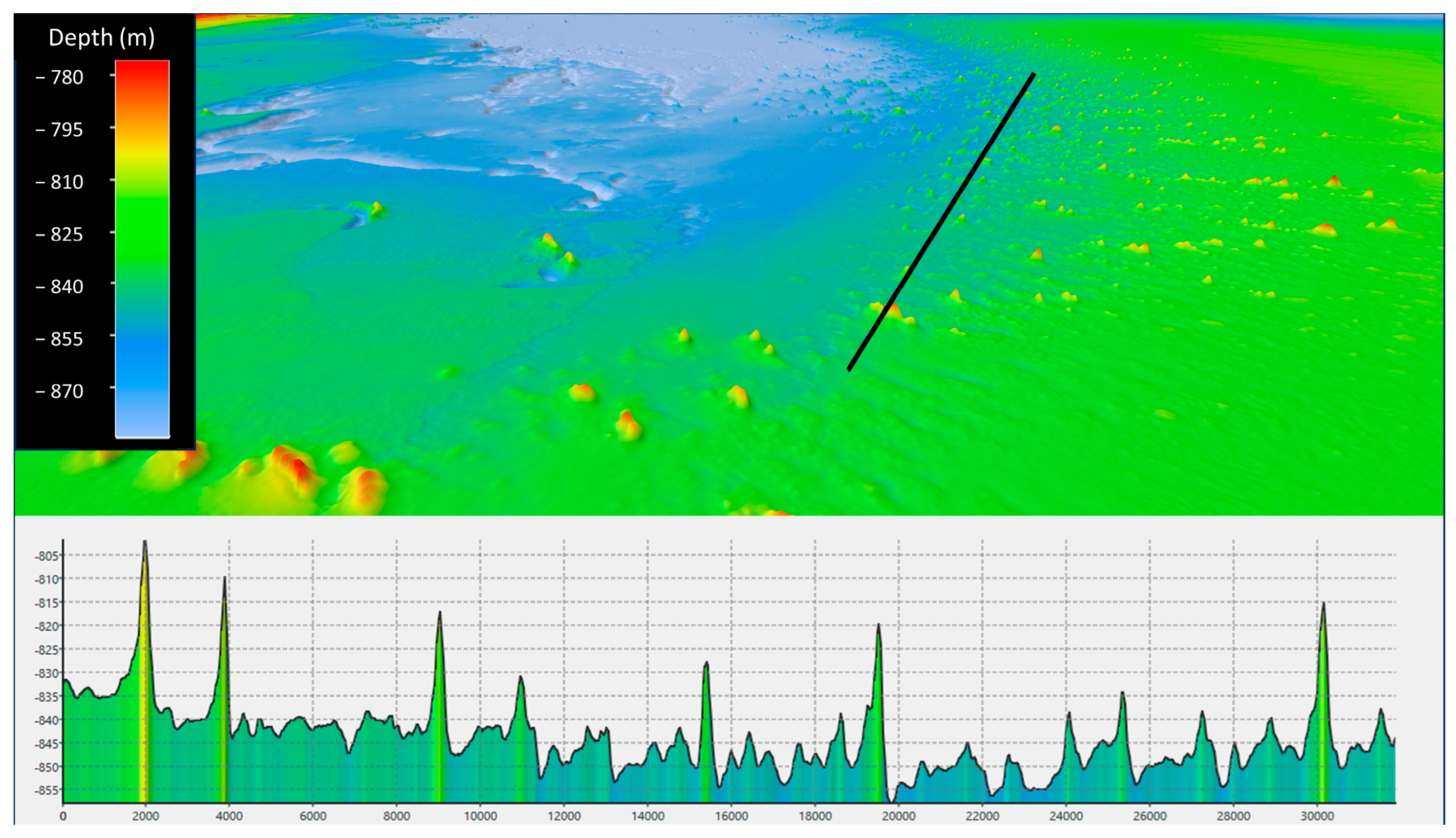
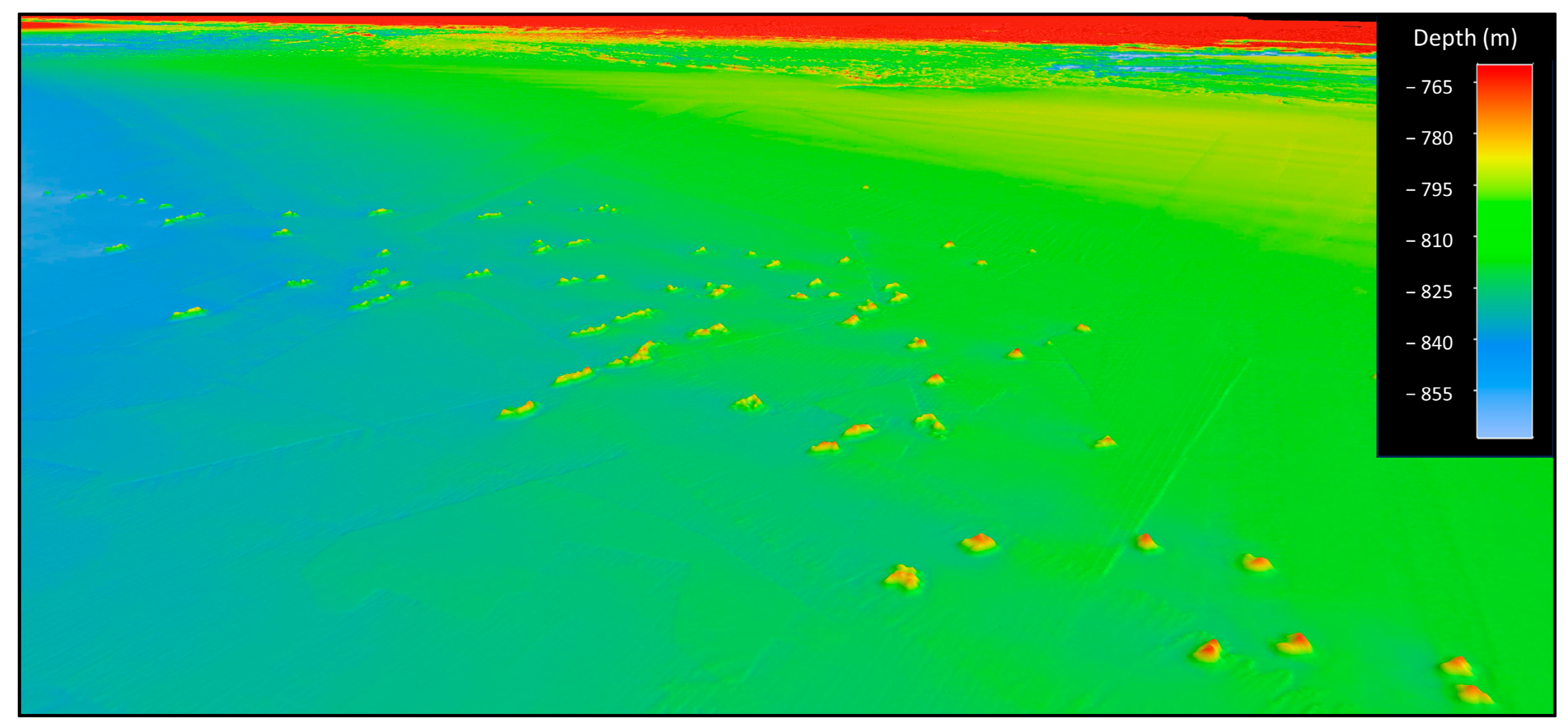
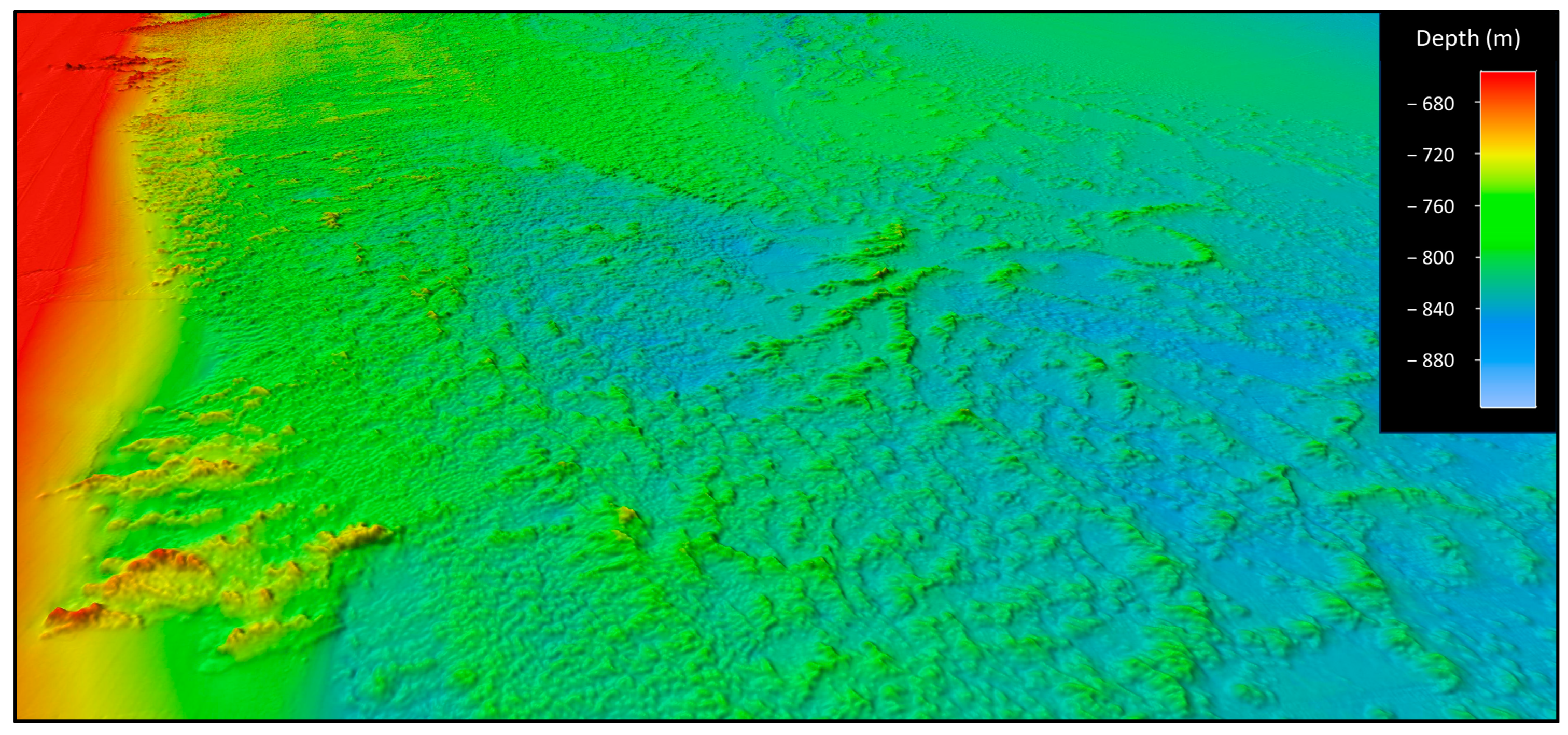
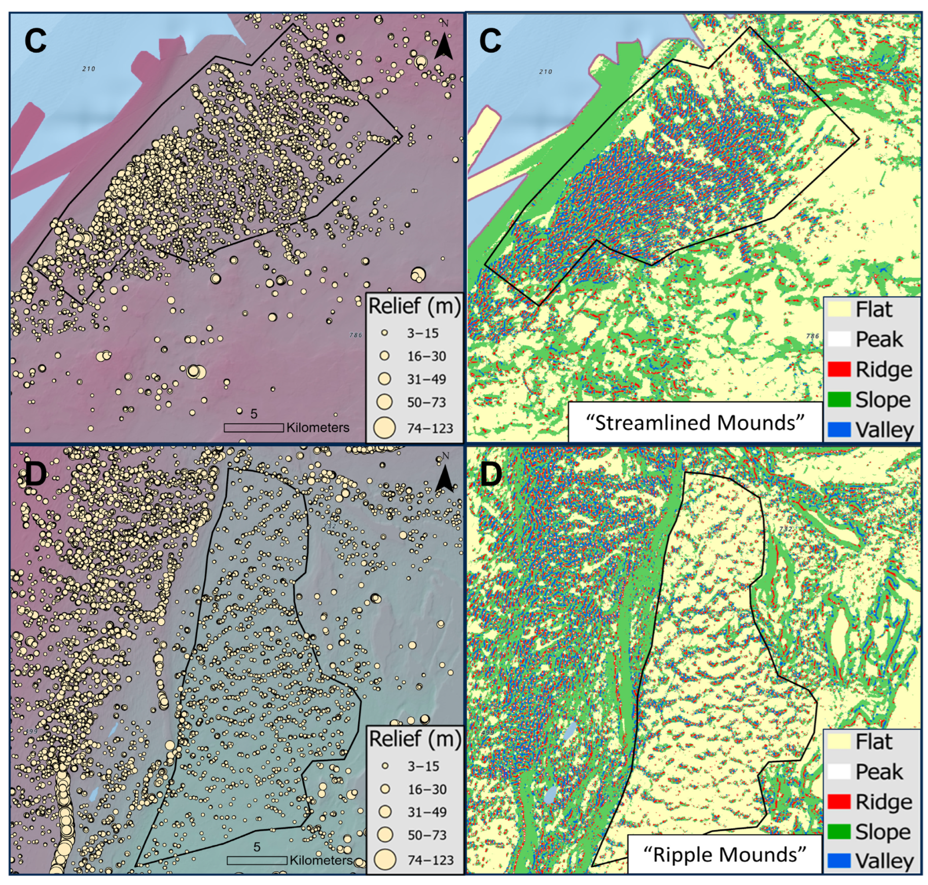
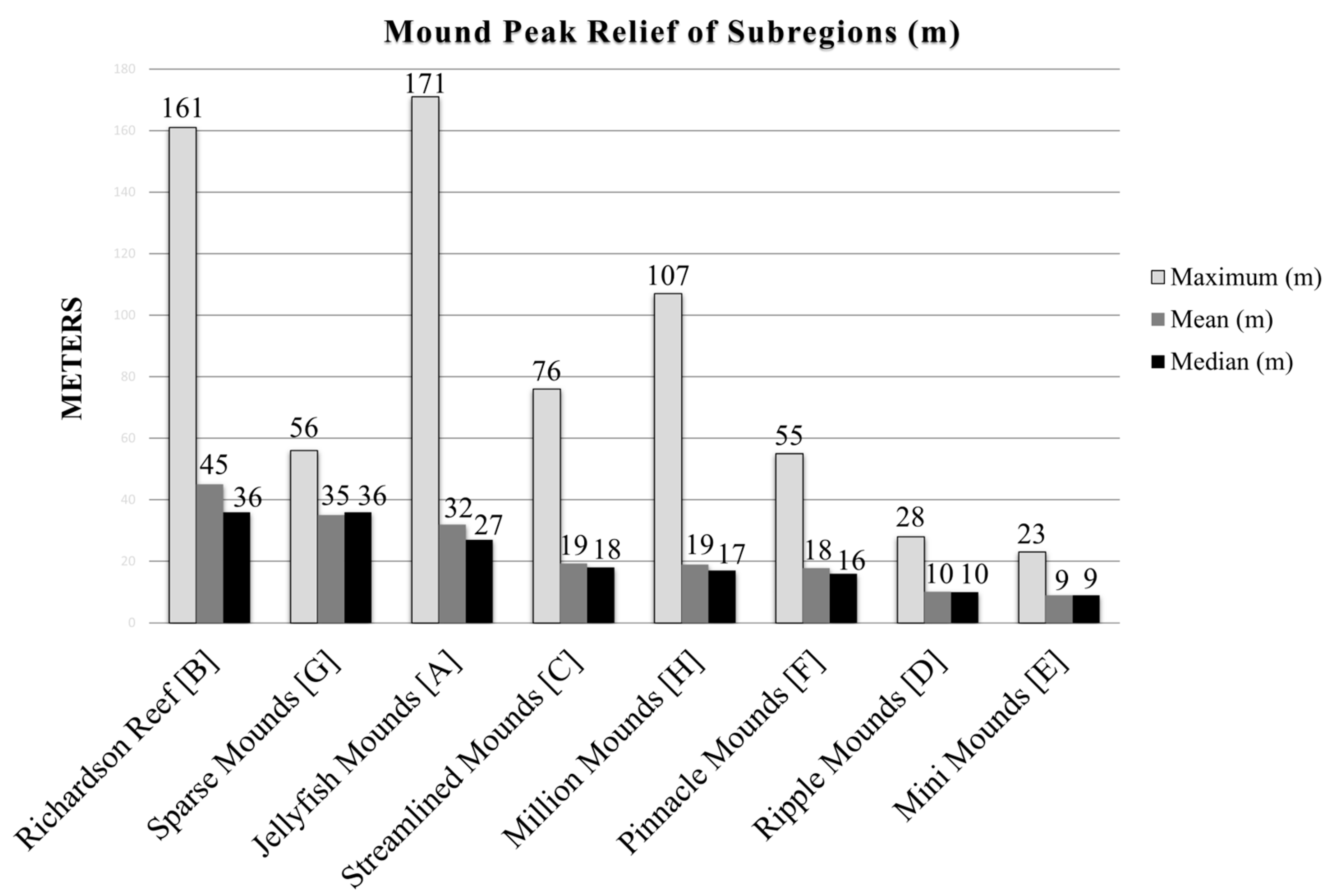
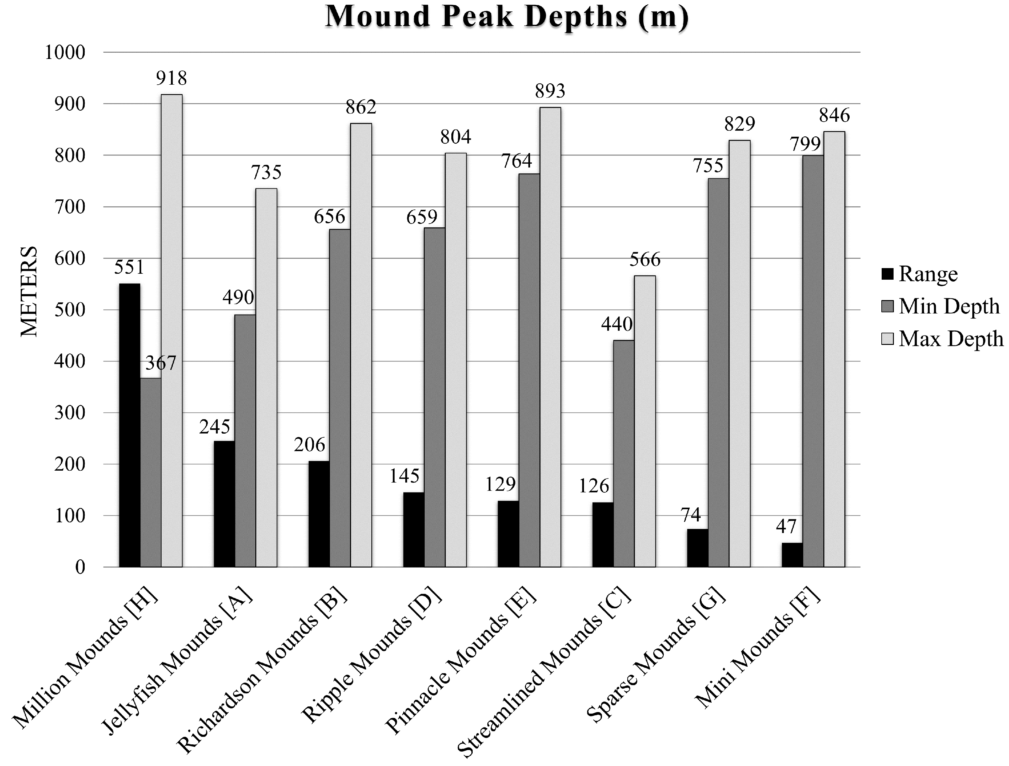
2.4. Geomorphic Analysis of Subregions and Mound Relief

Upon inspection of the geomorphology landforms layer of the Blake Plateau study area, it was readily apparent that there was a striking diversity of geomorphic patterns in the terrain that varied dramatically by subregion. The methods described in this section were used to characterize these geomorphic differences both qualitatively and quantitatively. To quantify differences of CWC mound characteristics across the Blake Plateau, additional spatial analysis was carried out using ArcGIS Pro v3.1.0.

The first step in the subregional characterization of CWC mound features was to subjectively select and delineate the subregions. Eight subregions of the overall study area were selected based on the following rationale:

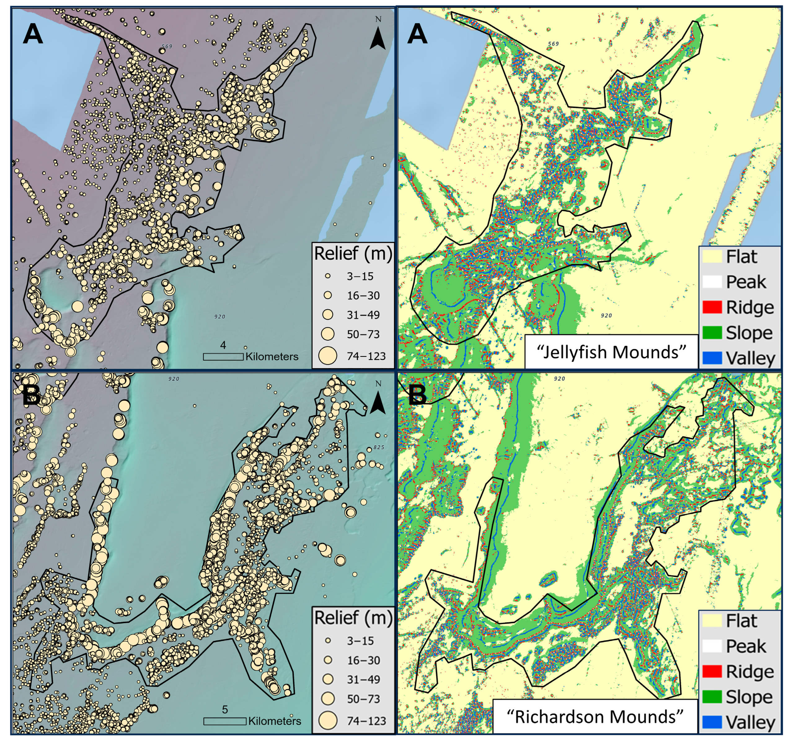
• Two were selected as examples of large mounds formed along the top of steep geologic scarp features of the terrain (“Jellyfish Mounds” and “Richardson Mounds”).
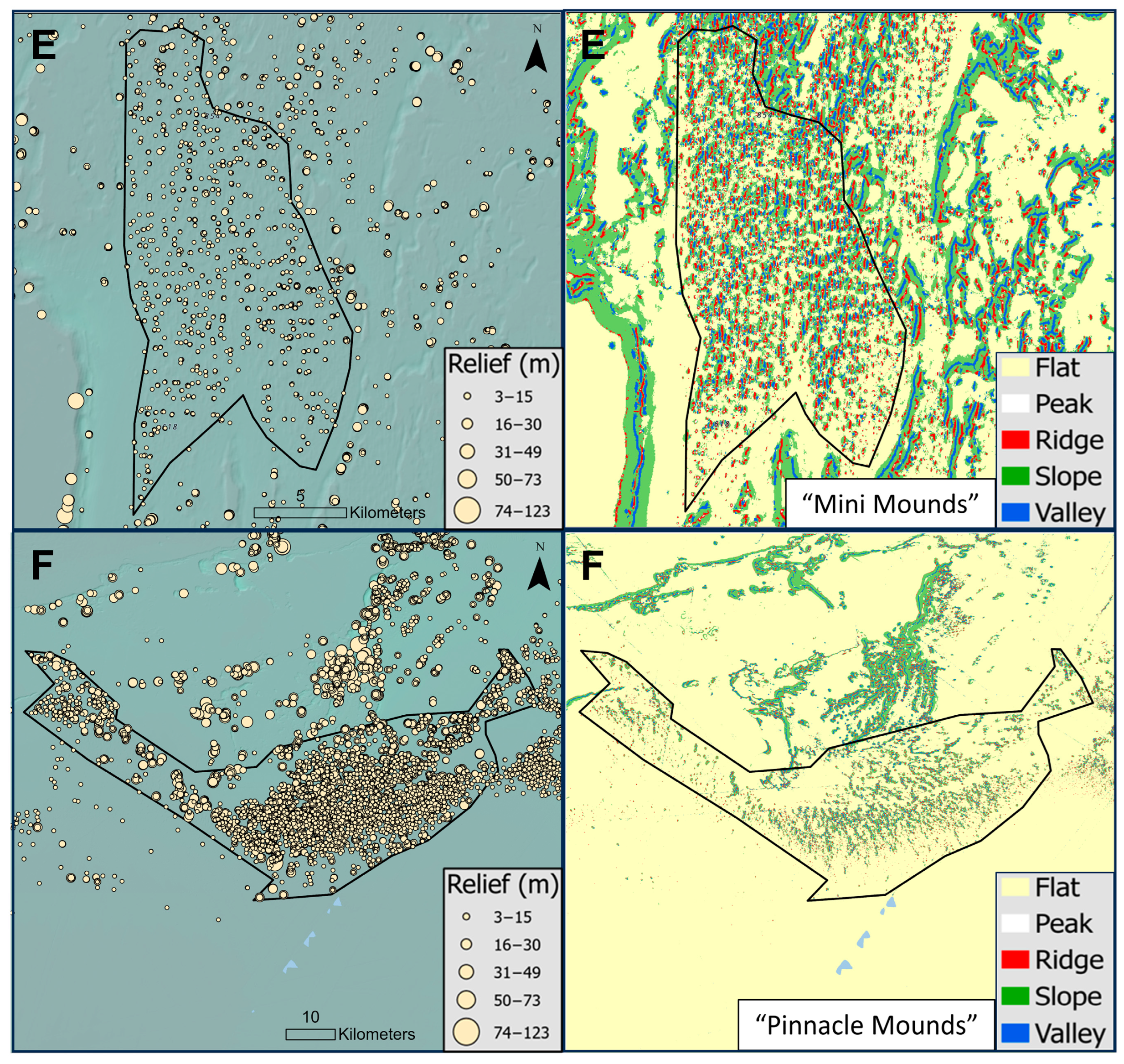
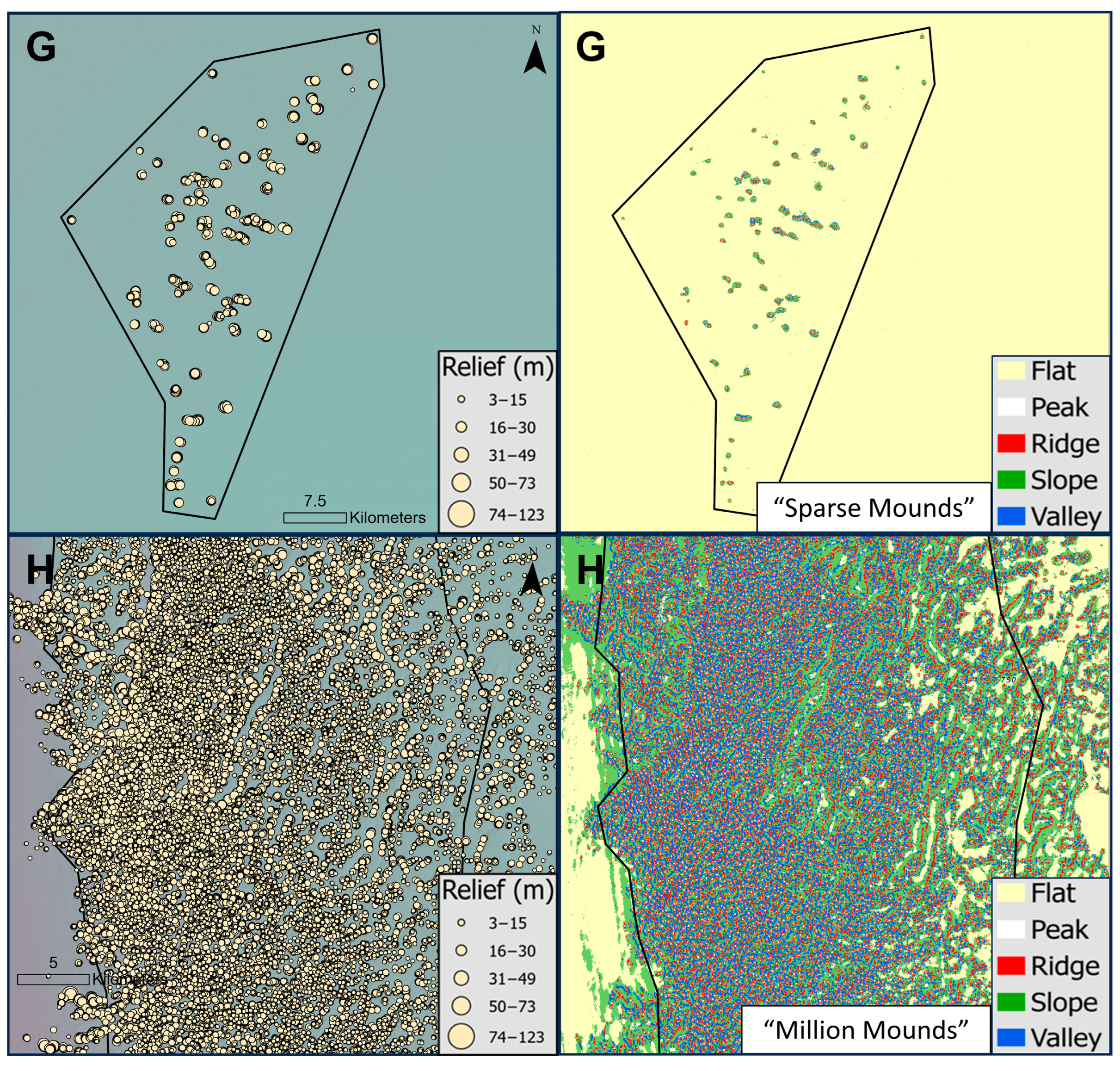
• Four subregions were selected based on their unique spatial pattern of mound features not observed elsewhere in the region (“Streamlined Mounds”, “Ripple Mounds”, “Mini Mounds”, and “Sparse Mounds”).
• One region was selected as a large newly mapped CWC mound area outside the existing coral Habitat Area of Particular Concern protection boundary (“Pinnacle Mounds”). Sparse Mounds also met this criterion.
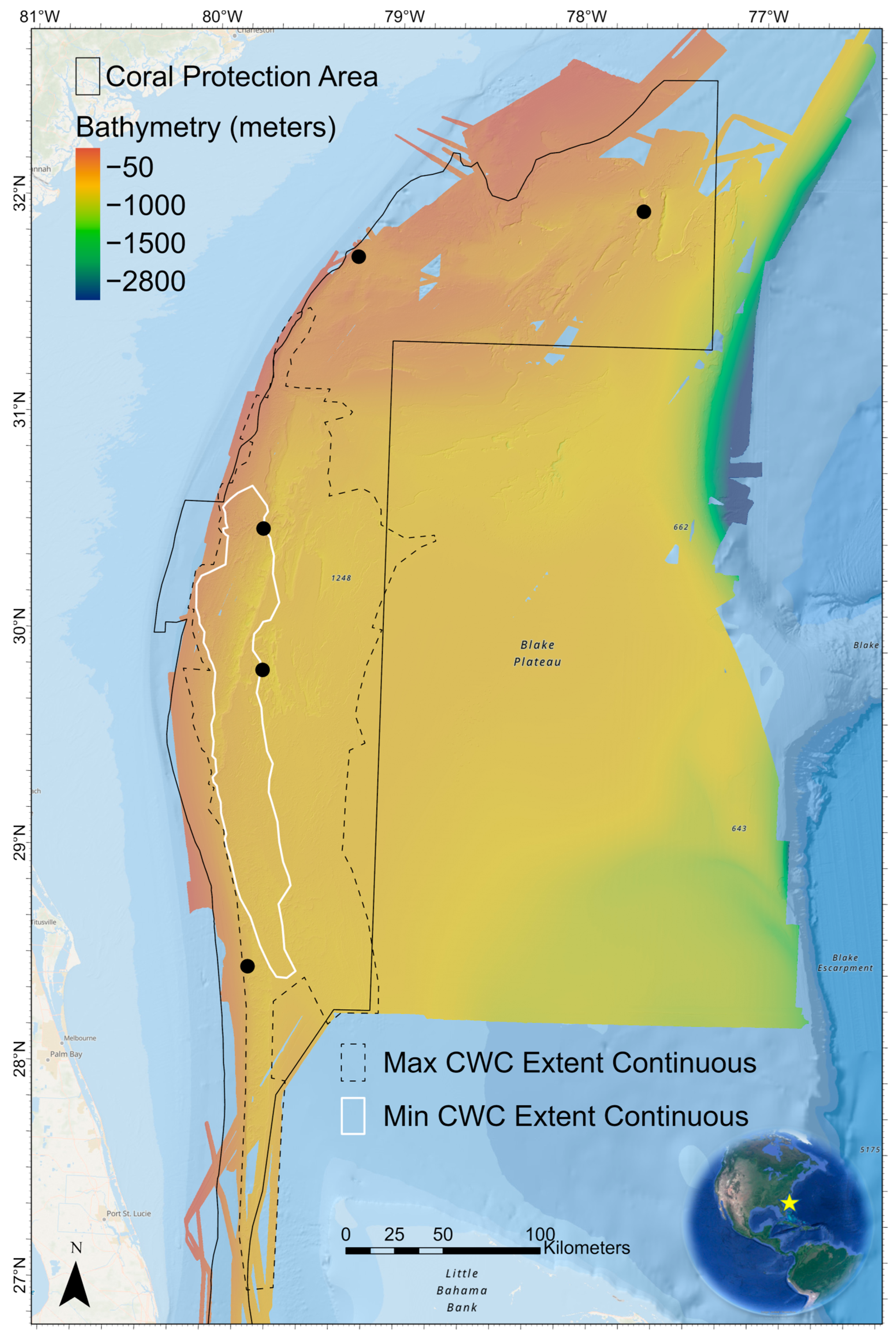
• One was selected for its exceptionally high mound densities over a large continuous spatial extent (“Million Mounds”). This area forms the core of the largest continuous extent of coral described in the paper (white polygon in Figure 2).

Bounding polygons for each of these eight areas were then hand-digitized in Arc using the bathymetry and landform layers to discriminate between areas of CWC mounds and surrounding flat terrain. To highlight the qualitative differences in landform patterns, oblique 3D and plan view figures were created for the eight subregions to visually display the diverse geomorphic “fingerprints” (i.e., pattern arrangement) of the landforms comprising each area. Landform pattern spatial layers were draped on the 3D bathymetry in QPS Fledermaus to enhance visualization.

Within each of the eight subregions the following metrics were calculated in ArcGIS Pro v3.1.0: number of mound peaks, peak density (number of peaks per km²), area of peak landforms, and mound peak minimum and maximum depths. To calculate these metrics, the vector layer of landform polygons was clipped to the subregion extent and the summary statistics tool was used to summarize the number of peak features and generate areas for peak and ridge landform classes. All areas were calculated using a geodesic formula to generate accurate area values undistorted by the map projection. To calculate the minimum and maximum depth of mound peak features, the “extract by mask” geoprocessing tool was used to mask the bathymetry layer with a vector layer of only peak landform features for each subregion. Minimum and maximum depth values were then noted for the resulting output raster.

The vertical relief of CWC mounds was deemed to be an important defining characteristic to quantify across the entire study area and within each subregion. Therefore, five metrics were calculated pertaining specifically to mound relief within each of these areas: minimum, maximum, mean, median, and standard deviation. In order to generate statistics of mound relief, a methodology was needed to calculate the approximate relief of any given mound feature from the surrounding terrain at the base of the mound.

The BRESS software can generate an optional statistical spatial layer output called “maximum height delta” that calculates the maximum change in height measured from any grid node to its surrounding visual neighborhood in eight line-of-sight directions. This calculation is limited to surrounding grid cells that fall within the user-specified inner and outer search radii parameters. The BRESS model run used to delineate landforms had inner and outer search radii set to 35 m and 210 m, respectively. While these radii parameters were optimized to effectively delineate CWC mound peak features, the outer radius of 210 m was not deemed adequate for calculating maximum height delta values because it truncated possible vertical relief values and resulted in underestimating the relief of mound features when compared with actual direct measurements of relief from the bathymetry of select test mounds. By direct measurement of the largest mounds in the bathymetry grid, a distance of 420 m was deemed able to capture the maximum vertical relief change from the top of any mound feature to the surrounding seafloor flats. Based on this, an additional model run of BRESS was completed on the bathymetric grid using an adjusted outer search radius value of 12 nodes (420 m) and the maximum height delta spatial output layer was saved and imported into ArcGIS Pro v3.1.0.

Mound relief values were calculated by using the subregional boundary polygons to clip the maximum height delta spatial layer in ArcGIS Pro. The result was a feature layer for each subregion that had individual polygons of only areas classified as peak landforms and attributed with values of maximum delta heights. The summary statistics geoprocessing tool was then run on this feature layer, querying for statistics on the sum of polygon areas, minimum, maximum, mean, median, and standard deviation. These values were then aggregated into a table of statistics from all subregions to enable comparisons.

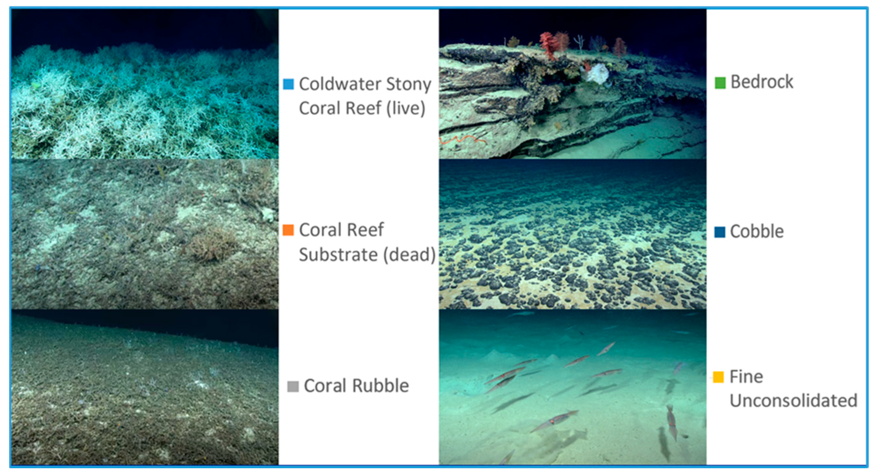
2.5. Substrate Classification and Comparison with Landforms

Video data recorded from 23 submersible dives were used to assess the substrate character within classified landforms: fifteen dives were completed using the dual-body Deep Discover/Seirios ROVs, four dives completed by HOV Alvin, and four dives by the dual-body Jason/Medea ROVs. Substrate observations from the dive videos were sub-sampled in some cases such that all dives had observations recorded at approximately one-minute time intervals while the vehicles were traversing terrain, resulting in 6081 substrate observations of the seafloor.

Twelve dives were annotated for primary (dominant) substrate at one-minute dive time intervals as part of detailed annotations for sessile fauna conducted for the DEEP SEARCH project. Five dives were annotated by NOAA OER staff using the same substrate types as DEEP SEARCH but also ensuring the decision criteria and substrate size thresholds followed the Coastal and Marine Ecological Classification Standard (CMECS). Six dives were annotated by staff at NOAA’s National Centers for Coastal Ocean Science Deep Coral Ecology Lab for primary substrates using a simplified CMECS terminology along with additional comment notes to provide more detail. These annotations were made for different purposes by different observers, but they were deemed general enough in nature to still be valid for the purposes of this study without cross-validation between different observers. For all observations, the terminology used to describe the primary dominant substrate type was harmonized with the standard terminology for primary substrate units published in CMECS. The “coldwater stony coral reef” unit is a biotic component descriptor in CMECS, but it was used in this study like a substrate class in order to differentiate living stony coral reef from dead standing coral-framework (dead stony coral skeletons not broken down into rubble).

Table 1. Substrate classification terminology used by the DEEP SEARCH team and how it was translated into standard terminology used in CMECS.

DEEP SEARCH Class	Relationship to CMECS	CMECS Class/Subclass	Relationship Notes
Live ScleractinianCoral	Nearly Equal (≈)	Coldwater Stony Coral Reef	Live vs. dead coral cannot be described with CMECS substrate classes; the Biotic Component Group unit for live coral was used.
Dead Standing Coral-framework	Less Than (<)	Coral Reef Substrate	CMECS unit is not as specific.
Coral Rubble	Equal (=)	Coral Rubble
Sediment	Greater than (>)	Fine Unconsolidated	Sediment in the DEEP SEARCH schema includes gravel classes. Anything smaller than cobble may be included, but gravel classes were rare in dive areas.
Sedimented Bedrock	Nearly Equal (≈)	Bedrock/Co-occurring element modifier Fine Unconsolidated	This class was used when the dominant substrate was clearly bedrock, but >50% had sediments thick enough to preclude most sessile reef-associated fauna.
Exposed Bedrock	Less Than (<)	Bedrock
Cobble	Nearly Equal (≈)	Cobble	Exact size thresholds unclear.

shows how substrate class terminology from DEEP SEARCH was converted to CMECS unit terminology. Figure 5 shows examples of video imagery stills of the common dominant substrate classes in the study area.

Each substrate observation was recorded with longitude, latitude, and depth information enabling accurate georeferencing. Excel files containing the substrate data for each dive were imported into ArcGIS Pro as point feature layers. Each layer was then queried to select by attribute each unique combination of primary substrate class and landform type. The number of point observations for each combination of substrate class (up to seven class possibilities) by each landform type (up to five possibilities: slope, peak, ridge, flat, and valley) was then entered into a separate Excel tracking sheet. Once these data were compiled for all 23 dives, total sums of substrate observations per landform class were computed and plotted as bar plots to summarize how substrate classes differed with landform type.

3. Results

3.1. Extent and Geomorphic Characterization of the Cold-Water Coral Province

Figure 2 shows the bathymetric synthesis of the whole study region, along with the polygon for the maximum extent of nearly continuous CWC mound features (dashed line black polygon) and the minimum extent core area of continuous CWC features (white polygon). Given the broad scale of Figure 2, individual CWC mounds cannot be seen. The maximum extent polygon is 500 km long from north to south and up to 110 km wide from west to east. The area enclosed is 26,064 km² (6.4 million acres). The core area of dense CWC mounds in the minimum extent polygon is 254 km long by up to 42 km wide, encompassing an area of 6215 km² (1.5 million acres).

The geomorphic landform classification of the bathymetry data using the BRESS terrain analysis tool enabled the quantification of 83,908 individual peak features, providing the first map-based overall estimate of the number of potential CWC mound features in the study region. Inspection of the peak landform class draped onto the bathymetry in QPS Fledermaus visualization software shows strong alignment with CWC mound peak features compared with expert interpretation and insights from submersible dives. This correlation means that the vast majority of features classified as peaks are indeed likely to be CWC mound peaks in this particular setting. An example oblique 3D view of the bathymetry grid and the landform classification results draped onto bathymetry is show in Figure 6.

Cumulative areas were calculated for each of the five geomorphic landform classes: peaks (411 km²), valleys (3598 km²), ridges (3642 km²), slopes (23,082 km²), and flats (102,848 km²). Figure 7 provides a bar graph of these results. While flats make up the largest area, the other four classes collectively cover an area of 30,733 km² and comprise the complex CWC mound and steep scarp features in the region. The aggregated area of peak features alone covers an area 7× the size of the island of Manhattan in New York City, and the area covered by peaks and ridges (where living corals are most likely to be found) together comprise an area larger than Yosemite National Park. Terrestrial protected area size comparisons are noted to prompt the reader to consider the ecosystem services provided by these important marine habitats at such a scale. These ecosystem services include carbon sequestration, nutrient regeneration, and biodiversity support, among others described in detail in a separate study focused on the Richardson Reef area [55]. A valuation of estimated ecosystem services for the Blake Plateau CWC mound province is beyond the scope of this study, but the initial characterization provided here provides a basis upon which further assessment can be undertaken.

The value of developing and applying a user-parameterized terrain segmentation and classification approach for geomorphic characterization becomes readily apparent in a massive and complex CWC mound province such as described here. As evident from Figure 6, manually delineating these features in a consistent repeatable way with a comparable level of detail would not be possible. Another benefit of this approach is the transparency of landform classification methods. Once the model is set up with a few user-defined parameters tailored to the study area, the algorithms are based on a published mathematical terrain modeling approach instead of expert judgment. Results can therefore be replicated by other researchers given the same input data and model parameters. The transparency of the BRESS modeling approach also enables it to be applied to other CWC provinces for more consistent comparative analysis.

Standardization of methods is an inherent objective of this study. The feasibility of using the geomorphic landform classes in order to classify “geoform” units as part of the CMECS standard was evaluated; therefore,

Table 2. Comparison of the geomorphic landform units classified in the current study to existing CMECS geoform unit terminology.

BRESS Landform Units from Study	CMECS Geoform Units Applicable to Study Area	Potential New CMECS Provisional Geoform Units
Peak	Closest analog is “Knob” but it is of geologic origin, not biogenic.	Mound Peak (if CWC mound) Scarp Peak (if on scarp feature)
Ridge	Ridge (no change)	Mound Ridge (if CWC mound)
Valley	Valley (current definition needs expansion beyond continental shelf)	Mound Valley (if adjacent to CWC mound) Scarp Valley (if at base of scarp feature)
Slope	Slope (no change)	Mound Slope (if CWC mound)
Flat	Flat (no change)	--
	Scarp/Wall Fault Scarp Erosion Scarp	--
	Deep/Cold-water Coral Reef Biogenic Deep Coral Reef (living) Deep Coral Carbonate Mound (Note this unit is comprised of “peak,” “ridge,” and “slope” landforms.)	New Level 2 units under CWC Reef Mound Peak Mound Ridge Mound Slope Mound Valley

provides a comparison of the landform units generated by this study versus the closest analogous geoform units in CMECS. Since CMECS is a dynamic content standard intended to be revised and updated over time, new provisional units may be proposed. New potential provisional geoform units are listed in column three of Table 2. If the proposed units existed in CMECS, the landform classes from this study could largely be transitioned 1:1 to a standardized terminology scheme.

The high-resolution bathymetric synthesis and objectively generated full-coverage spatial geomorphology layers generated by this study offer strong potential as a valuable input into coral habitat suitability models of the region. Many species of cold-water corals show particular affinities for high-relief hard substrate features found on mound peaks and ridges. Utilizing fine scale delineations of these features as model inputs—or weighted spatial filters for fine tuning output probabilities—may result in more accurate models with improved predictive performance.

3.2. Geomorphic Diversity of Subregions

The complex geomorphology of eight subregions is characterized in this section qualitatively with geomorphic “fingerprints” and quantitatively by measurements of mound density and vertical relief. The median mound relief for the entire study region was 16 m, with individual mound features ranging 3–226 m above the adjacent seafloor. Figure 8 provides an overview map of the landform classification results for the entire study area and highlights the locations of the featured subregions. Subregions are labeled A-H and were provided an informal site name for the purposes of this study. Informal names do not correspond to any officially named features in the region. Richardson Reef/Mounds and Million Mounds are colloquial names used by some scientists and managers in the region.

Three-dimensional views of the bathymetry for each of the subregions (A–H) are shown to provide a visual contrast of the diversity of mound pattern formation and density across the Blake Plateau. Jellyfish Mounds (A) are shown below in Figure 9. Richardson Mounds (B) have already been shown above in Figure 1. Subregions C–G are shown in Figure 10, Figure 11, Figure 12, Figure 13 and Figure 14. The central region of the large Million Mounds subregion (H) is shown in Figure 6, and the southern region of Million Mounds is shown in Figure 15. All bathymetry grids shown are 35 m resolution and projected to WGS84, UTM 18N.

Additional maps of each subregion are provided in Figure 16, Figure 17, Figure 18 and Figure 19. The left panels display graduated symbols of mound relief overlain on hill-shaded bathymetry, with each circle representing an individual mound feature. The larger the beige circle, the greater the vertical relief of the mound. These maps quickly provide a visual display of mound densities and relative relief across the bathymetric grid. The right panels display the unique spatial patterns of geomorphic landform classes of the subregions (“fingerprints”) and provide an immediate visual contrast between flat areas and complex terrain. Letters in the top left corner correspond to the letters in the Figure 8 overview map. Black outlines in the figures are the polygons delineated for the purpose of quantifying and contrasting metrics about the nature of mounds in each subregion.

A review of Figure 16, Figure 17, Figure 18 and Figure 19 provides some interesting qualitative insights into the diversity of CWC mound morphologies in this region. In Figure 16, both Jellyfish (A) and Richardson Mounds (B) show obvious patterns of high relief mound features formed at the tops and edges of the steep scarps found in that subregion. Jellyfish Mounds are located at the northwest edge of Richardson Mounds. The linearity and continuity of the mound features along the distinct ridges found at the top of the scarp features are different from other parts of the Blake Plateau where mound features do not form in lines and have more space between each other.

Streamlined Mounds (C) in Figure 17 shows extremely high mound densities and tight clustering. In stark contrast, the Ripple Mounds subregion (D) in Figure 17 shows mounds linearly aligned along widely spaced gently curving crest patterns. The mound features are found on minor topographic highs spaced roughly 800–2000 m apart. It is unclear if this pattern of mound development is a result of the corals populating existing minor crests in the bathymetry with favorable substrates, or if the pattern was created via spatial self-organization through scale-dependent feedbacks [56]. This particular pattern is unique to this subregion of the Blake Plateau.

Another unique pattern is found in the Mini Mounds subregion (E) as shown in Figure 18. The mounds here are remarkably uniform in spacing and in their diminutive height, with an average vertical relief of 9 m. These mounds are also elongated in a roughly north–south orientation. The Pinnacle Mounds subregion (F) is a sprawling area (50 km wide) of newly mapped CWC habitats encompassing areas of dense mounds of fairly uniform size as well as more widely spaced mounds of larger size.

The Sparse Mounds subregion (G) in Figure 19 exhibits unique characteristics, showing widely spaced but prominent mounds in an otherwise very flat region of the Blake Plateau. There is no surface terrain expression of favorable underlying geology in the Sparse Mounds area. This observation is in contrast to other subregions such as Jellyfish and Richardson that have CWC mounds that have formed along the tops of geological scarp features that must have provided favorable circumstances to sustain the growth of stony corals.

The Million Mounds (H) subregion in Figure 19 is a remarkable standout from all other regions in terms of the sheer number and high densities of its mounds. This area is directly underneath the main axis of the Gulf Stream, and it is therefore subject to very consistent strong currents and delivery of suspended particles as a food source. Based on field experience, the currents here also make it a challenging place to obtain high quality multibeam sonar data and conduct safe submersible dives.

Pinnacle Mounds (F) and Sparse Mounds (G) are large newly discovered regions of CWC mounds located outside of the existing Stetson-Miami HAPC protection zone. Sparse Mounds contain some of the highest relief mounds on the plateau, and ROV exploration here revealed large areas of coral rubble, dense live Desmophyllum reef, and patches of Madrepora corals—documenting the high biological importance of these CWC mound features. The 2433 mounds in area F and 228 mounds in area G represent large newly discovered CWC habitats of major significance meriting consideration of additional conservation measures and study.

Within each of the eight subregions, the following metrics were calculated in ArcGIS Pro v3.1.0 to characterize CWC mound features: number of mound peaks, peak density (number of peaks per km²), area of peak landforms, and mound peak minimum and maximum depths. Additional statistics were also calculated specific to CWC mound feature relief from the surrounding terrain: minimum, maximum, mean, median, and standard deviation. These values were then aggregated into a table of statistics from all subregions to enable comparisons (

Table 3. Comparison of morphology metrics for the eight CWC mound subregions evaluated.

Mound Subregion Name	# of Peaks	Peak Density (#/km2)	Area of Peaks (km2)	Mound Relief Metrics					Mound Peak Min Depth (m)	Mound Peak Max Depth (m)
				Min (m)	Max (m)	Mean (m)	Median (m)	Std. Dev. (m)
A. Jellyfish	1043	3.1	7.1	3	171	32	27	20.8	490	735
B. Richardson	1342	2.8	7.7	3	161	45	36	32.5	656	862
C. Streamlined	1626	4.8	8.1	3	76	19	18	8.7	440	566
D. Ripple	833	2.6	3.7	3	28	10	10	3.5	659	804
E. Mini	554	2.7	1.8	4	23	9	9	3.1	799	846
F. Pinnacle	2443	1.2	13.8	2	55	18	16	9.5	764	893
G. Sparse	228	0.2	1.8	4	56	35	36	8.5	755	829
H. Million	35,789	5.8	186.3	3	107	19	17	10.2	367	918
Entire Region	83,908	0.8	411	0	226	20	16	13.4	168	2707

).

Within the overall study region, 83,908 individual peak features were identified. Mound relief within subregions ranged from 3 to 171 m above adjacent seafloor within the 420 m radius used to calculate relief. The Million Mounds subregion polygon (H) contained 35,789 individual mound features—43% of the total number of mounds mapped in the entire region. Peak density (5.8 mounds/km²) and the area of peaks (186.3 km²) were also greatest in Million Mounds. Note that the extended interpretation of the Million Mounds continuous CWC region (“max CWC extent continuous” polygon in Figure 2) contains 64,706 mound features (representing 77% of the total on the Blake Plateau). Streamlined Mounds had the second-highest peak density (4.8 mounds/km²), and it is clearly a distinctive area in this respect. Million Mounds supports the largest depth range of coral mound features (551 m), with some mounds as shallow as 367 m and as deep as 918 m. Mound peak relief maximum, mean, and median values for each subregion are plotted in Figure 20.

Mound features along the tops of geologic scarps (Jellyfish and Richardson) had the highest relief values, followed by Million Mounds and Streamlined Mounds. It has already been noted that mound features located at the top of steep scarp features show high terrain relief, so the maximum values are subject to significant change depending on the polygon subregion location and inclusion of specific mound features. High relief values alone do not provide insight into the proportion of relief due to the elevation of the underlying biogenic structure (formed by stony coral skeletons and sediment deposition over long time scales) versus the base geology that any given mound formed upon. Therefore, the maximum relief values should be interpreted cautiously, while still providing some utility in terms of comparing subregion values. Sparse and Pinnacle Mounds had essentially the same maximum values. Ripple Mounds and Mini Mounds had the lowest maximum relief.

Richardson Mounds has the highest mean and median relief values, but it is closely followed by Sparse Mounds and then Jellyfish Mounds. It is apparent that while the Sparse Mounds subregion does not have a great number of mounds, the mounds that are present are on average some of the tallest in the region, with a mean value of 35 m and a median value of 36 m. Streamlined, Million, and Pinnacle Mounds all have mean and median values within 1–2 m of each other, which is interesting because these areas also have the highest overall number of mounds out of the subregions evaluated. These numbers demonstrate that the Pinnacle Mounds area has similar characteristics to existing regions within the HAPC boundary. Ripple and Mini Mounds subregions have the smallest average relief at 10 m and 9 m, respectively. The standard deviation provides a measure of how diverse the range of mound relief is within each subregion. Richardson has the highest diversity of mound relief, followed by Jellyfish—not surprising given the large scarps in these regions.

The depth values for mound peak features within each subregion are displayed in Figure 21. All of the mound peaks in the subregions fall within the depth range of 367–918 m. The greatest variation in mound depths is within the Million Mounds area, spanning a range of 551 m. Both the shallowest (367 m) and deepest (918 m) mound depths are also found in the Million Mounds subregion. All other subregions have considerably narrower depth ranges. Sparse Mounds and Mini Mounds had the smallest ranges at 74 and 47 m, respectively. Mini, Pinnacle, and Sparse Mounds were the deepest overall areas—with their shallowest mound peaks at 799 m, 764 m, and 755 m, respectively. The deeper sites may be important climate refuge areas for stony corals and reefs in the region as temperatures in deep waters continue to increase in the future [31].

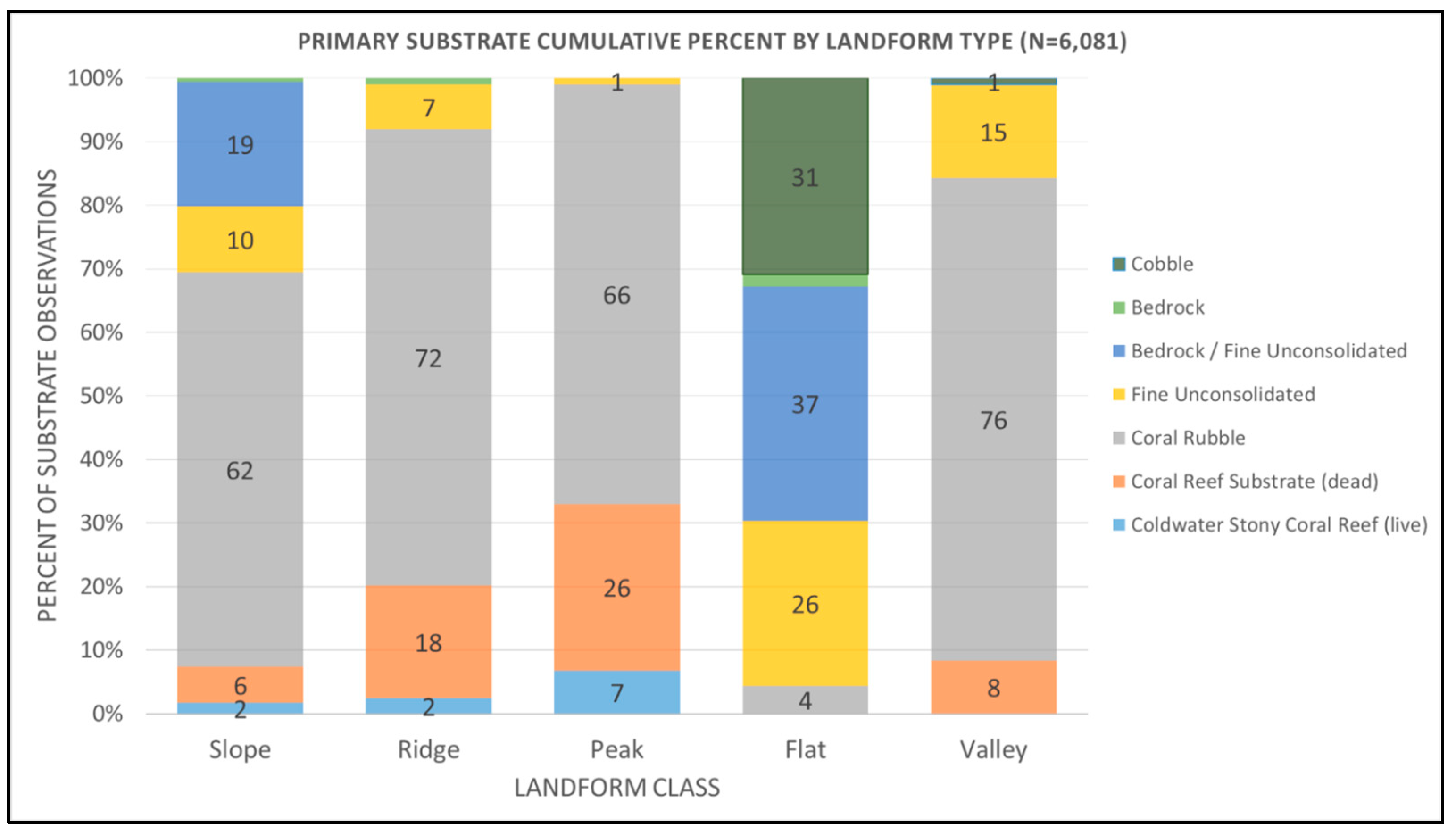
3.3. Substrate Classes of Landform Types

Substrate observations recorded from video data from 23 submersible dives at approximately 1 min intervals (n = 6081 substrate annotations) were harmonized with CMECS terminology and used to assess the substrate character within classified landforms. Slope features had the greatest number of overall observations, followed by ridges and peaks. Given that the CWC mound features were the target of most dives, it is logical that most of the observations occurred traversing up the slope, followed by exploration of the ridges and peaks of the mounds. Flat and valley landforms only represent 9% and 6%, respectively, of the overall observations. A cumulative bar plot of the results is shown in Figure 22.

As evident from the cumulative plot shown in Figure 22, coral rubble (shown in gray) was found to be the dominant substrate component within the peak (66%), ridge (72%), and slope (62%) landforms, thereby validating the interpretation of these bathymetric features as CWC mounds. This result was true even on mounds with as little as 10 m of average vertical relief from the surrounding seafloor, as documented for the Ripple Mounds and Mini Mounds subregions.

Live stony coral reef (light blue) was found exclusively on peaks (7%), ridges (2%), and slopes (2%). This is in agreement with recent habitat suitability modeling completed in the region, in which the bathymetric position index and slope were the top two variables for predicting live coral occurrence [31]. Dead coral reef substrate (i.e., dead standing coral-framework) is shown in orange and was also found almost exclusively on peaks (26%), ridges (18%), and slopes (6%)—with more standing framework typically found in the higher relief areas. Unconsolidated sediments (shown in yellow) are mostly absent from peaks (1%) but do occur sporadically on ridges (7%) and slopes (10%). The substantial coral rubble component in the valleys (76%) may indicate that rubble is conveyed downslope by strong currents, biodegradation, and gravity to accumulate in certain valley features adjacent to mounds. It is notable that cobble (dark green, 31%) and bedrock (light green and dark blue classes, 2% and 37% respectively) were major components of the flats explored—evidence of the hard-bottom habitats in the region. The majority of bedrock observed was covered in fine sediments (>50%) as a co-occurring element (CMECS class bedrock/fine unconsolidated).

The “rubble” class in this study should not be interpreted as corals damaged by human activities. Rubble substrate in the context of this study area occurs naturally as a result of the gradual breakdown of dead coral-framework. Coral rubble can support high faunal diversity [16] and is therefore an important marine habitat. Direct evidence of damage to coral and rubble habitats was not a component of this study. Numerous studies have clearly documented the sensitivity of CWC mound habitat (including rubble) to bottom-contact fishing practices or other human activities [22,57,58]. The substrate data in this study was methodically translated to CMECS terminology, with the intention that this will improve the longevity and usefulness of the data in the longer term.

4. Discussion and Conclusions

This study demonstrated the value of applying an objective automated terrain segmentation and classification approach to geomorphic characterization of a highly complex CWC mound province. Manual delineation of these features in a consistent repeatable way with a comparable level of detail would not have been possible. As inevitably larger regions of the oceans become mapped and explored, and the technological capability to map extensive seafloor features in high resolution with autonomous underwater vehicles (AUVs) expands, the importance of semi-automated classification approaches will only increase. Reliance solely on manual delineation and expert judgment is not a practical approach in these circumstances, and the inability to reproduce results and standardize methods across large ocean regions further supports the need for standardization or at least transparency in methodologies and terminology. The methods used in this study provide a pragmatic standardized approach for identifying, characterizing, and quantifying CWC mound-forming habitats and could be applied to other CWC provinces to enable more direct comparisons among geographically diverse settings.

The multibeam sonar bathymetric compilation and corresponding geomorphic landform maps generated by this study document what appears to be the most extensive CWC mound province thus far discovered (see [14] for a summary of other known CWC mound provinces). Nearly continuous CWC mound features span an area up to 500 km long and 110 km wide, covering an area of 26,064 km² (Figure 2). Within this area, there is a core area of exceptionally high-density mounds up to 254 km long by 42 km wide, covering an area of 6215 km² (Subregion H, Million Mounds). To put the size of these areas in perspective with terrestrial protected areas in the U.S., the CWC province extent is almost 3× larger than Yellowstone National Park and the core area of very dense mounds is larger than Grand Canyon National Park or Everglades National Park.

A total of 83,908 individual peak features were delineated, providing the first estimate of the overall number of potential CWC mounds mapped in the region to date. Five geomorphic landform classes were mapped and quantified covering the entire study area: peaks (411 km²), valleys (3598 km²), ridges (3642 km²), slopes (23,082 km²), and flats (102,848 km²).

CWC mound spatial distribution, density, vertical relief, and morphology varied greatly among subregions of the Blake Plateau. The mean mound peak relief above the surrounding seafloor for the entire study region was 20 m (median value was 16 m), with individual mound features in analyzed subregions ranging between 3 and 171 m in vertical relief. Two large areas containing prominent and numerous CWC mounds (Pinnacle and Sparse Mounds) were mapped and characterized that exist outside the present-day Stetson-Miami Habitat Area of Particular Concern. The northern area (Pinnacle) has 2443 mound features and the southern area (Sparse) has 228.

The direct alignment of the Florida Current/Gulf Stream Current with the underlying most dense and extensive CWC mound province (Subregion H, Million Mounds) provides clear evidence of how important this current regime is in delivering nutrients and determining the spatial extent of mound formation. The relationship between CWC mound size and flow hydrodynamics is complex and in need of additional research [21,59] with important ramifications for the suitability of mounds for supporting stony coral growth and associated biota [56]. The CWC mound relief spatial layers and summary statistics generated in this study, along with habitat suitability modeling [31], can be used to target study sites for assessing hydrodynamic relationships with CWC mounds of diverse sizes across the Blake Plateau province. The relative ages of CWC mound features across the plateau are also currently unknown.

The quantification of mound landform features provides a more robust basis to assess the significance of the ecosystem services provided by this major CWC province. Characterization of the Blake Plateau CWC mound province extent and geomorphic diversity is of direct relevance to marine resource managers charged with implementing ecosystem-based management approaches and protecting vulnerable seafloor habitats from potentially harmful human impacts. Based on the methodology presented in this study, there are 7782 potential CWC mounds located outside of the existing Stetson/Miami Terrace Deep Water Coral Habitat Area of Particular Concern (HAPC) boundary established to protect corals.

Ground-truth data for the geoform analysis were provided by direct substrate observations from 23 submersible dive videos that revealed coral rubble to be the dominant substrate component within the peak, ridge, and slope landforms explored, thereby validating the interpretation of these bathymetric features as CWC mounds. These results infer that it is reasonable to expect about 99% of classified mound peak areas and 92% of classified mound ridge areas to have a dominant substrate type that is CWC-related (coral rubble, dead coral-reef substrate, and a small component of live cold-water stony coral reef). This has important implications for the collective ecological value of this CWC mound province given the proven linkages between coral habitat (live and dead) and the benthic and pelagic communities shown to be associated with them. These CWC-based habitats support rich communities of associated invertebrates and fishes in the Blake Plateau region [15,47,55,60]. Submersible dive video data are biased towards under-sampling of the substrate characteristics of flat and valley features (9% and 6%, respectively, of the overall substrate observations), and therefore the data presented in this study for these geomorphic features may not be adequately representative of these habitats.

The application of the Coastal and Marine Ecological Classification Standard (CMECS) in deep-sea environments is still evolving, and recommendations for interim provisional units were provided for the geoform component of the standard. The existing substrate classification units worked well for this study.

The extent and nature of CWC mounds characterized in this study should be compared with the other largest reported CWC mound and reef areas discovered thus far. The Røst Reef in Norway has previously been recognized as the largest known CWC (Desmophyllum pertusum) reef, with an extent of 35 km × 3 km wide [61,62] and covering an area of approximately 100 km² [63]. The Mauritanian CWC mound province consists primarily of dead coral mounds that span a nearly continuous line of mound features 400 km long, but with a narrow width and an unreported total area of coverage [30]. The West Florida slope mounds reported by Reed et al. [15] span an area of 230 km long by 10 km wide. The Northern Argentine Mound Province is estimated to cover an area at least 2000 km² [64]. In comparison with these published studies, the core area of dense CWC mounds in the minimum extent polygon delineated in this study for the Million Mounds subregion alone covers a nearly continuous area of 6215 km² and is larger in extent than any other continuous CWC mound or reef province yet discovered and published in the scientific literature. The results of this study provide essential information to enable comparisons with other CWC mound provinces in order to understand the global characteristics of this ecologically critical marine habitat.

While the Blake Plateau region has been recognized since the 1960s as one of the world’s most significant CWC mound areas, the full extent and geomorphic diversity of these critical coral habitats has now been revealed as a direct result of the strategic multi-year, multi-partner ocean exploration campaign summarized in this article.

References

1. Roberts, J.M.; Wheeler, A.J.; Freiwald, A. Reefs of the deep: The biology and geology of cold-water coral ecosystems. Science 2006, 312, 543–547. [Google Scholar] [CrossRef]
2. Mayer, L.; Jakobsson, M.; Allen, G.; Dorschel, B.; Falconer, R.; Ferrini, V.; Lamarche, G.; Snaith, H.; Weatherall, P. The Nippon Foundation—GEBCO Seabed 2030 Project: The Quest to See the World’s Oceans Completely Mapped by 2030. Geosciences 2018, 8, 63. [Google Scholar] [CrossRef]
3. de Carvalho Ferreira, M.L.; Robinson, L.F.; Stewart, J.A.; Li, T.; Chen, T.; Burke, A.; White, N.J. Spatial and temporal distribution of cold-water corals in the Northeast Atlantic Ocean over the last 150 thousand years. Deep. Sea Res. Part I Oceanogr. Res. Pap. 2022, 190, 103892. [Google Scholar] [CrossRef]
4. Lunden, J.J.; McNicholl, C.G.; Sears, C.R.; Morrison, C.L.; Cordes, E.E. Acute survivorship of the deep-sea coral Lophelia pertusa from the Gulf of Mexico under acidification, warming, and deoxygenation. Front. Mar. Sci. 2014, 1, 78. [Google Scholar] [CrossRef]
5. Georgian, S.E.; Shedd, W.; Cordes, E.E. High-resolution ecological niche modelling of the coldwater coral Lophelia pertusa in the Gulf of Mexico. Mar. Ecol. Prog. Ser. 2014, 506, 145–161. [Google Scholar] [CrossRef]
6. Quattrini, A.M.; Nizinski, M.S.; Chaytor, J.D.; Demopoulos, A.W.; Roark, E.B.; France, S.C.; Moore, J.A.; Heyl, T.; Auster, P.J.; Kinlan, B. Exploration of the Canyon-Incised Continental Margin of the Northeastern United States Reveals Dynamic Habitats and Diverse Communities. PLoS ONE 2015, 10, e0139904. [Google Scholar] [CrossRef]
7. Wheeler, A.J.; Beyer, A.; Freiwald, A.; De Haas, H.; Huvenne, V.A.; Kozachenko, M.; Olu-Le Roy, K.; Opderbecke, J. Morphology and environment of cold-water coral carbonate mounds on the NW European margin. Int. J. Earth Sci. 2007, 96, 37–56. [Google Scholar] [CrossRef]
8. Genin, A.; Dayton, P.K.; Lonsdale, P.F.; Spiess, F.N. Corals on seamount peaks provide evidence of current acceleration over deep-sea topography. Nature 1986, 322, 59–61. [Google Scholar] [CrossRef]
9. Messing, C.; Neumann, A.; Lang, J. Biozonation of Deep-Water Lithoherms and Associated Hardgrounds in the Northeastern Straits of Florida. Palaios 1990, 5, 15–33. [Google Scholar] [CrossRef]
10. Reed, J.K. Comparison of deep-water coral reefs and lithoherms off southeastern USA. Hydrobiologia 2002, 471, 57–69. [Google Scholar] [CrossRef]
11. Stetson, T.R.; Squires, D.F.; Pratt, R.M. Coral banks occurring in deep water on the Blake Plateau. Am. Mus. Nat. Hist. 1962, 2114, 1–39. [Google Scholar]
12. Neumann, A.C.; Ball, M.M. Submersible observations in the Straits of Florida: Geology and bottom currents. Geol. Soc. Am. Bull. 1970, 81, 2861–2874. [Google Scholar] [CrossRef]
13. Freiwald, A.; Fosså, J.H.; Grehan, A.; Koslow, T.; Roberts, J.M. Cold-Water Coral Reefs; UNEP-WCMC: Cambridge, UK, 2004. [Google Scholar]
14. Cordes, E.E.; Mienis, F.; Gasbarro, R.; Davies, A.; Baco, A.R.; Bernardino, A.F.; Clark, M.; Freiwald, A.; Hennige, S.; Huvenne, V.A.I.; et al. A Global View of the Cold-Water Coral Reefs of the World. In The Cold-Water Coral Reefs of the World; Cordes, E.E., Mienis, F., Eds.; Springer: Berlin/Heidelberg, Germany, 2024; pp. 1–30. [Google Scholar]
15. Reed, J.K.; Weaver, D.C.; Pomponi, S.A. Habitat and fauna of deep-water Lophelia pertusa coral reefs off the southeastern U.S.: Blake plateau, Straits of Florida, and Gulf of Mexico. Bull. Mar. Sci. 2006, 78, 343–375. [Google Scholar]
16. Roberts, J.M.; Wheeler, A.; Freiwald, A.; Cairns, S. Cold-Water Corals: The Biology and Geology of Deep-Sea Coral Habitats; Cambridge University Press: Cambridge, UK, 2009; p. 367. [Google Scholar]
17. Cordes, E.E.; McGinley, M.P.; Podowski, E.L.; Becker, E.L.; Lessard-Pilon, S.; Viada, S.T.; Fisher, C.R. Coral communities of the deep Gulf of Mexico. Deep.-Sea Res. Part I-Oceanogr. Res. Pap. 2008, 55, 777–787. [Google Scholar] [CrossRef]
18. Henry, L.A.; Roberts, J.M. Global Biodiversity in Cold-Water Coral Reef Ecosystems. In Marine Animal Forests; Rossi, S., Bramanti, L., Gori, A., Orejas Saco del Valle, C., Eds.; Springer: Cham, Switzerland, 2016. [Google Scholar] [CrossRef]
19. Mortensen, P.B.; Hovlund, M.; Brattegard, T.; Farestveit, R. Deep water bioherms of the scleractinian coral Lophelia pertusa (L.) at 64o N on the Norwegian shelf: Structure and associated megafauna. Sarsia 1995, 80, 145–158. [Google Scholar] [CrossRef]
20. Jones, C.G.; Lawton, J.H.; Shachak, M. Organisms as ecosystem engineers. Oikos 1994, 69, 373–386. [Google Scholar] [CrossRef]
21. Soetaert, K.; Mohn, C.; Rengstorf, A.; Grehan, A.; van Oevelen, D. Ecosystem engineering creates a direct nutritional link between 600-m deep cold-water coral mounds and surface productivity. Sci. Rep. 2016, 6, 35057. [Google Scholar] [CrossRef] [PubMed]
22. Fosså, J.; Mortensen, P.; Furevik, D. The deep-water coral Lophelia pertusa in Norwegian waters: Distribution and fishery impacts. Hydrobiologia 2002, 471, 1–12. [Google Scholar] [CrossRef]
23. Cordes, E.E.; Jones, D.O.B.; Schlacher, T.A.; Amon, D.J.; Bernardino, A.F.; Brooke, S.; Carney, R.; DeLeo, D.M.; Dunlop, K.M.; Escobar-Briones, E.G. Environmental Impacts of the Deep-Water Oil and Gas Industry: A Review to Guide Management Strategies. Front. Environ. Sci. 2016, 4, 58. [Google Scholar] [CrossRef]
24. Parker, S.; Penney, A.; Clark, M. Detection criteria for managing trawl impacts on vulnerable marine ecosystems in high seas fisheries of the South Pacific Ocean. Mar. Ecol. Prog. Ser. 2009, 397, 309–317. [Google Scholar] [CrossRef]
25. Grasmueck, M.; Eberli, G.P.; Viggiano, D.A.; Correa, T.; Rathwell, G.; Luo, J. Autonomous underwater vehicle (AUV) mapping reveals coral mound distribution, morphology, and oceanography in deep water of the Straits of Florida. Geophys. Res. Lett. 2006, 33, L23616. [Google Scholar] [CrossRef]
26. Kilgour, J.M.; Auster, P.J.; Packer, D.; Purcell, M.; Packard, G.; Dessner, M.; Sherrell, A.; Rissolo, D. Use of AUVs to Inform Management of Deep-Sea Corals. Mar. Technol. Soc. J. 2014, 48, 21–27. [Google Scholar] [CrossRef]
27. Angeletti, L.; Castellan, G.; Montagna, P.; Remia, A.; Taviani, M. The Corsica Channel cold-water coral province. Front. Mar. Sci. 2020, 7, 661. [Google Scholar] [CrossRef]
28. Hebbeln, D.; Wienberg, C.; Wintersteller, P.; Freiwald, A.; Becker, M.; Beuck, L.; Dullo, C.; Eberli, G.P.; Glogowski, S.; Matos, L. Environmental forcing of the Campeche cold-water coral province, southern Gulf of Mexico. Biogeosciences 2014, 11, 1799–1815. [Google Scholar] [CrossRef]
29. Taviani, M.; Angeletti, L.; Canese, S.; Cannas, R.I.; Cardone, F.; Cau, A.N.; Cau, A.B.; Follesa, M.C.; Marchese, F.; Montagna, P. The Sardinian cold-water coral province in the context of the Mediterranean coral ecosystems. Deep Sea Res. Part II Top. Stud. Oceanogr. 2017, 145, 61–78. [Google Scholar] [CrossRef]
30. Wienberg, C.; Titschack, J.; Freiwald, A.; Frank, N.; Lundälv, T.; Taviani, M.; Beuck, L.; Schröder-Ritzrau, A.; Krengel, T.; Hebbeln, D. The giant Mauritanian cold-water coral mound province: Oxygen control on coral mound formation. Quat. Sci. Rev. 2018, 185, 135–152. [Google Scholar] [CrossRef]
31. Gasbarro, R.; Sowers, D.; Margolin, A.; Cordes, E.E. Distribution and predicted climatic refugia for a reef-building cold-water coral on the southeast US margin. Glob. Change Biol. 2022, 28, 7108–7125. [Google Scholar] [CrossRef] [PubMed]
32. Hain, S.; Corcoran, E. The status of the cold-water coral reefs of the world. In Status of Coral Reefs of the World; Wilkinson, C., Ed.; Australian Institute of Marine Science: Perth, Australia, 2004; pp. 115–135. [Google Scholar]
33. Partyka, M.L.; Ross, S.W.; Quattrini, A.M.; Sedberry, G.R.; Birdsong, T.W.; Potter, J.; Gottfried, S. Southeastern United States Deep-Sea Corals (SEADESC) Initiative: A Collaborative Effort to Characterize Areas of Habitat-Forming Deep-Sea Corals; NOAA Technical Memorandum OAR OER 1; National Oceanic and Atmospheric Administration: Silver Spring, MD, USA, 2007.
34. Reed, J.K.; Messing, C.; Walker, B.K.; Brooke, S.; Correa, T.B.; Brouwer, M.; Udouj, T.; Farrington, S. Habitat characterization, distribution, and areal extent of deep-sea coral ecosystems off Florida, Southeastern USA. Caribb. J. Sci. 2013, 47, 13–30. [Google Scholar] [CrossRef]
35. Ross, S.W.; Nizinski, M.S. State of deep coral ecosystems in the U.S. Southeast Region: Cape Hatteras to Southeastern Florida. In The State of Deep Coral Ecosystems of the United States; Lumsden, S.E., Hourigan, T.F., Bruckner, A.W., Dorr, G., Eds.; NOAA Technical Memorandum CRCP 3; National Oceanic and Atmospheric Administration: Silver Spring, MD, USA, 2007; pp. 239–269. [Google Scholar]
36. Zibrowius, H. Les Scléractiniaires de la Méditerranée et de l’Atlantique nord-oriental. Mémoires De L’institut Océanographique Monaco 1980, 11, 1–284. [Google Scholar]
37. Larcom, E.A.; McKean, D.L.; Brooks, J.M.; Fisher, C.R. Growth rates, densities, and distribution of Lophelia pertusa on artificial structures in the Gulf of Mexico. Deep. Sea Res. Part I Oceanogr. Res. Pap. 2014, 85, 101–109. [Google Scholar] [CrossRef]
38. Galvez, K.C. The Distribution and Growth Patterns of Cold-Water Corals in the Straits of Florida. Ph.D. Thesis, University of Miami, Coral Gables, FL, USA, 2020. [Google Scholar]
39. Ayers, M.W.; Pilkey, O.H. Piston cores and surficial sediment investigations of the Florida-Hatteras slope and inner Blake Plateau. In Environmental Geologic Studies on the Southeastern Atlantic Outer Continental Shelf; Popenoe, P., Ed.; USGS Open File Report 81-582-A; U.S. Geological Survey: Reston, VI, USA, 1981; pp. 5-1–5-89. Available online: https://pubs.usgs.gov/of/1981/0582a/report.pdf (accessed on 2 November 2023).
40. SAFMC. Deepwater Coral HAPCs. South Atlantic Fisheries Management Council. Available online: https://safmc.net/managed-areas/deep-water-coral-hapcs/ (accessed on 2 November 2023).
41. Wagner, D.; Etnoyer, P.J.; Schull, J.C.; Nizinski, M.S.; Hickerson, E.L.; Battista, T.A.; Netburn, A.N.; Harter, S.L.; Schmahl, G.P.; Coleman, H.; et al. Science Plan for the Southeast Deep Coral Initiative (SEDCI), 2016–2019; NOAA Technical Memorandum NOS NCCOS 230; National Oceanic and Atmospheric Administration: Charleston, SC, USA, 2017; p. 96. Available online: https://coastalscience.noaa.gov/data_reports/science-plan-for-the-southeast-deep-coral-initiative-sedci-2016-2019/ (accessed on 2 November 2023).
42. Cordes, E. #DEEPSEARCH. Temple University. Available online: https://sites.temple.edu/cordeslab/research/dep-search/ (accessed on 8 January 2024).
43. FGDC-STD-018-2012; Coastal and Marine Ecological Classification Standard. FGDC (Federal Geographic Data Committee): Reston, VA, USA, 2012.
44. Baringer, M.O.; Larsen, J.C. Sixteen years of Florida Current transport at 27° N. Geophys. Res. Lett. 2001, 28, 3179–3182. [Google Scholar] [CrossRef]
45. Richardson, P.L. Florida Current, Gulf Stream, and Labrador Current. Encycl. Ocean. Sci. 2001, 2, 1054–1064. [Google Scholar]
46. Hogg, N.G.; Johns, W.E. Western boundary currents. U.S. National Report to International Union of Geodesy and Geophysics 1991–1994. Suppl. Rev. Geophys. 1995, 33, 1311–1334. [Google Scholar] [CrossRef]
47. Ross, S.W. Review of distribution, habitats, and associated fauna of deep water coral reefs on the southeastern United States Continental Slope (North Carolina to Cape Canaveral, FL). S. Atl. Fish. Manag. Counc. Rep. 2006, 1, 1–36. [Google Scholar]
48. Masetti, G.; Mayer, L.A.; Ward, L.G. A bathymetry- and reflectivity-based approach for seafloor segmentation. Geosciences 2018, 8, 14. [Google Scholar] [CrossRef]
49. Sowers, D.; Dijkstra, J.A.; GMasetti, G.; Mayer, L.A.; Mello, K.; Malik, M. Application of the Coastal and Marine Ecological Classification Standard to Gosnold Seamount, North Atlantic Ocean. In Seafloor Geomorphology as Benthic Habitat: Geohab Atlas of Seafloor Geomorphic Features and Benthic Habitat, 2nd ed.; Elsevier Inc.: Amsterdam, The Netherlands, 2019; p. 1076. [Google Scholar]
50. Sowers, D.C.; Masetti, G.; Mayer, L.A.; Johnson, P.; Gardner, J.V.; Armstrong, A.A. Standardized Geomorphic Classification of Seafloor within the United States Atlantic Canyons and Continental Margin. Front. Mar. Sci. 2020, 7, 9. [Google Scholar] [CrossRef]
51. Dolan, M.F.; Bjarnadóttir, L.R. Highlighting broad-scale morphometric diversity of the seabed using geomorphons. GEUS Bull. 2023, 52, 8337. [Google Scholar] [CrossRef]
52. Jasiewicz, J.; Stepinski, T.F. Geomorphons—A pattern recognition approach to classification and mapping of landforms. Geomorphology 2013, 182, 147–156. [Google Scholar] [CrossRef]
53. Hydroffice. Bathymetric- and Reflectivity-Based Estimator of Seafloor Segments (BRESS). Available online: https://www.hydroffice.org/bress/main (accessed on 2 November 2023).
54. Walbridge, S.; Slocum, N.; Pobuda, M.; Wright, D.J. Unified Geomorphological Analysis Workflows with Benthic Terrain Modeler. Geosciences 2018, 8, 94. [Google Scholar] [CrossRef]
55. Cordes, E.E.; Demopoulos, A.W.J.; Davies, A.J.; Gasbarro, R.; Rhoads, A.C.; Lobecker, E.; Sowers, D.; Chaytor, J.D.; Morrison, C.L.; Weinnig, A.M. Expanding our view of the cold-water coral niche and accounting of the ecosystem services of the reef habitat. Sci. Rep. 2023, 13, 19482. [Google Scholar] [CrossRef]
56. Van der Kaaden, A.S.; Mohn, C.; Gerkema, T.; Maier, S.R.; de Froe, E.; van de Koppel, J.; van Oevelen, D. Feedbacks between hydrodynamics and cold-water coral mound development. Deep. Sea Res. Part I Oceanogr. Res. Pap. 2021, 178, 103641. [Google Scholar] [CrossRef]
57. Grehan, A.J.; Unnithan, V.; Olu-Le Roy, K.; Opderbecke, J. Fishing impacts on Irish deepwater coral reefs: Making a case for coral conservation. In: Barnes PW, Thomas JP (eds) Benthic habitats and the effects of fishing. Am. Fish. Soc. Symp. 2005, 41, 819–832. [Google Scholar]
58. Koslow, J.A.; Boehlert, G.W.; Gordon, J.D.M.; Haedrich, R.L.; Lorance, P.; Parin, N. Continental slope and deep-sea fisheries: Implications for a fragile ecosystem. ICES J. Mar. Sci. 2000, 57, 548–557. [Google Scholar] [CrossRef]
59. Cyr, F.; van Haren, H.; Mienis, F.; Duineveld, G.; Gourgault, D. On the influence of cold-water coral mound size on flow hydrodynamics, and vice versa. Geophys. Res. Lett. 2016, 43, 775–783. [Google Scholar] [CrossRef]
60. Ross, S.W.; Quattrini, A.M. The fish fauna associated with deep coral banks off the southeastern United States. Deep. Sea Res. Part I Oceanogr. Res. Pap. 2007, 54, 6. [Google Scholar] [CrossRef]
61. Fosså, J.H.; Lindberg, B.; Christensen, O.; Lundälv, T.; Svellingen, I.; Mortensen, P.B.; Alvsvåg, J. Mapping of Lophelia reefs in Norway: Experiences and survey methods. In Cold-Water Corals and Ecosystems; Freiwald, A., Roberts, J.M., Eds.; Springer: Berlin/Heidelberg, Germany, 2005; pp. 359–391. [Google Scholar]
62. ICES. Report of the ICES Advisory Committee on Ecosystems, 2002. ICES Coop. Res. Rep. 2002, 254, 129. [Google Scholar]
63. World Wildlife Fund. The Røst Reef—A Potential MPA. Available online: https://wwf.panda.org/our_work/our_focus/oceans_practice/coasts/coral_reefs/ (accessed on 10 October 2020).
64. Steinmann, L.; Baques, M.; Wenau, S.; Schwenk, T.; Spiess, V.; Piola, A.R.; Bozzano, G.; Violante, R.; Kasten, S. Discovery of a giant cold-water coral mound province along the northern Argentine margin and its link to the regional Contourite Depositional System and oceanographic setting. Mar. Geol. 2020, 427, 106223. [Google Scholar] [CrossRef]
Figure 1. Example of what CWC mounds can look like in multibeam sonar bathymetry data. This oblique 3D perspective figure shows the bathymetry of the Richardson Mounds subregion of the Blake Plateau. Prominent CWC mounds are found along the top edges of the geological scarp features in continuous linear chains. CWC mounds can also form in linear patterns or as more randomized bumps in the seafloor not associated with scarp features as also shown here. The interpretation of these features as CWC mounds was verified in this area using both ROV and HOV dives. Image created in QPS Fledermaus software (V7.8.12) with 4× vertical exaggeration.
Geomatics 04 00002 g001
Figure 2. Bathymetric terrain model synthesis grid of the Blake Plateau CWC mound study region from 31 different multibeam sonar surveys. The white polygon represents the minimum extent core area of dense nearly continuous CWC mound features in the largest CWC province on the plateau. The yellow star on the inset map represents the location of the Blake Plateau adjacent to the southeast U.S. coastline. The black dotted line polygon represents the maximum extent of continuous CWC features in the largest province. There are many other subregions on the plateau with CWC mounds. The solid black polygon shows the existing boundaries of the Stetson-Miami Deepwater Coral Habitat Area of Particular Concern. At this scale, individual coral mound features are not discernible. The numbered black point features on the map correspond to the locations of some of the previous study locations described on the Blake Plateau: 1—Stetson Banks [10,11], 2—Savannah Banks [46], 3—Jacksonville Lithoherms [10], 4—St. Augustine [15], and 5—Cape Canaveral Pinnacles [15]. The map projection is WGS 84/UTM zone 18N (EPSG:32618), and the background is ESRI’s ocean basemap.
Geomatics 04 00002 g002
Figure 3. A 3D view example of how input bathymetry data is classified into 5 different landform types using BRESS. The bathymetry and vertical relief of a typical mound feature is shown on the left, and the automatically classified landform features from BRESS (draped onto the bathymetry) are shown on the right.
Geomatics 04 00002 g003
Figure 4. Summary workflow diagram of the steps used in this study to complete the geomorphic classification of the Blake Plateau.
Geomatics 04 00002 g004
Figure 5. Primary (dominant) substrate classes used in the study. CMECS unit terminology is shown.
Geomatics 04 00002 g005
Figure 6. Oblique perspective 3D views of a section of the core area of dense mounds in the central portion of the “Million Mounds” subregion. Bathymetry of mound features in meters (upper panel). Geomorphic landform classification draped onto the bathymetry (lower panel). Resolution of grids is 35 m and vertical exaggeration of 7×. The white line is the minimum extent polygon of continuous mound features, and the black line is the maximum extent polygon. Note the delineation of the white peak features from the rest of the CWC mounds (inset) to enable the enumeration of mounds and the calculation of mound relief metrics for each mound. Data visualization using QPS Fledermaus software.
Geomatics 04 00002 g006
Figure 7. Bar plot showing the cumulative areas of the five geomorphic landform classes within the overall study region.
Geomatics 04 00002 g007
Figure 8. Geomorphic landform overview map with subregions labeled AH: Jellyfish Mounds (A); Richardson Mounds (B); Streamlined Mounds (C); Ripple Mounds (D); Mini Mounds (E); Pinnacle Mounds (F); Sparse Mounds (G); and Million Mounds (H). All subregions contain CWC mound features. Note how the landform map provides a strong immediate visual contrast between flat areas and complex terrain. Black circles show the location of submersible dives with video footage of the seafloor used to ground-truth substrates. The yellow star on the inset map represents the location of the Blake Plateau adjacent to the southeast U.S. coastline.
Geomatics 04 00002 g008
Figure 9. Oblique perspective 3D view of Jellyfish Mounds (subregion A), with vertical exaggeration of 4×. Some residual sound speed artifacts in the multibeam sonar data are visible in the bathymetry grid (e.g., striping in the top left quadrant of the figure), but most of the mound features shown are real terrain features.
Geomatics 04 00002 g009
Figure 10. Oblique perspective 3D view of Streamlined Mounds (subregion C), with vertical exaggeration of 4×. These mounds show clear directionality in mound orientation. Mounds are elongated along the southwest-to-northeast direction, indicating a very likely strong morphology-shaping influence of the consistently strong Gulf Stream current in this area.
Geomatics 04 00002 g010
Figure 11. Oblique perspective 3D view of Ripple Mounds (subregion D), with vertical exaggeration of 4×. These mounds are among the smallest in the region (3–28 m relief), and their spatial pattern is unique on the Blake Plateau.
Geomatics 04 00002 g011
Figure 12. Oblique perspective 3D view of Mini Mounds (subregion E), with vertical exaggeration of 4×. Mound sizes are comparable to Ripple Mounds, but they are located 50 km away and exhibit a much different spatial pattern.
Geomatics 04 00002 g012
Figure 13. A 3D oblique perspective view of the 35 m resolution bathymetry for the Pinnacle Mounds (subregion F) subregion (top panel) with 4× vertical exaggeration. The bottom panel shows a profile of mound relief with vertical exaggeration of 533 corresponding to the black line in the top panel. Mounds here tend to be single standalone pointy features, which is in contrast to other areas that have either elongated asymmetrical shapes or mounds composed of compound features with several peaks.
Geomatics 04 00002 g013
Figure 14. Oblique perspective 3D view of Sparse Mounds (subregion G), with vertical exaggeration of 4×. These isolated mounds are located on a large flat expanse of the Blake Plateau 50 km east of the Million Mounds subregion and 60 km south of the Pinnacle Mounds subregion. While there are only 228 mound peak features here, they are among the tallest on the plateau and the ROV dive completed on one of the mounds documented the highest percent cover (up to 80.4%) of live Desmophyllum pertusum coral reef out of all of the submersible dives in the study. This area is located outside of the current HAPC boundary.
Geomatics 04 00002 g014
Figure 15. Oblique perspective 3D view of the southern portion of the Million Mounds (subregion H) subregion, with vertical exaggeration of 4×. Note the sheer number and density of mounds here, and the distinct western edge around 700 m depth where the mounds cease.
Geomatics 04 00002 g015
Figure 16. Maps showing graduated vertical mound relief symbols (left panels) and landform classifications (right panels) for Jellyfish Mounds (subregion A) and Richardson Mounds (subregion B).
Geomatics 04 00002 g016
Figure 17. Maps showing graduated vertical mound relief symbols (left panels) and landform classifications (right panels) for Streamlined Mounds (subregion C) and Ripple Mounds (subregion D).
Geomatics 04 00002 g017
Figure 18. Maps showing graduated vertical mound relief symbols (left panels) and landform classifications (right panels) for Mini Mounds (subregion E) and Pinnacle Mounds (subregion F).
Geomatics 04 00002 g018
Figure 19. Maps showing graduated vertical mound relief symbols (left panels) and landform classifications (right panels) for Sparse Mounds (subregion G) and Million Mounds (subregion H). Given the large size of the Million Mounds subregion, only a portion of it is shown in the figure. Note the extreme density of mounds in area H, which are the highest in the overall study area.
Geomatics 04 00002 g019
Figure 20. CWC mound peak relief of eight subregions based on the maximum vertical change in any of the eight directions up to 420 m radius surrounding a peak landform feature. The maximum single vertical relief value within a subregion is shown in orange. Yellow bars represent mean values and green bars represent median values of all peaks in the subregion. The subregions are ordered by largest to smallest mean relief values moving from left to right along the x-axis.
Geomatics 04 00002 g020
Figure 21. Bar plot showing depths of CWC mound peak features in each subregion. The range of peak depths is shown in green, minimum depths are shown in orange, and maximum depths are shown in yellow. The subregions are ordered by largest to smallest depth range values moving from left to right along the x-axis.
Geomatics 04 00002 g021
Figure 22. Plot of primary substrate types observed for each landform class based on interpretation of submersible video data. The y-axis represents the cumulative percent of substrate observations aggregated for each landform class.
Geomatics 04 00002 g022