Article

Feasibility of Using Green Laser in Monitoring Local Scour around Bridge Pier

by
Rahul Dev Raju
1,*,
Sudhagar Nagarajan
2,
Madasamy Arockiasamy
2 and
Stephen Castillo
2
1
Department of Ocean and Mechanical Engineering, Florida Atlantic University, Boca Raton, FL 33431, USA
2
Department of Civil, Environmental and Geomatics Engineering, Florida Atlantic University, Boca Raton, FL 33431, USA
*
Author to whom correspondence should be addressed.
Geomatics 2022, 2(3), 355-369; https://doi.org/10.3390/geomatics2030020
Submission received: 20 June 2022 / Revised: 4 August 2022 / Accepted: 29 August 2022 / Published: 4 September 2022

Abstract

:
Scour around bridge piers is considered as one of the major factors which causes failure of bridges in the United States. An undetected scour can affect the stability of the bridge, eventually leading to the collapse of the bridge. The experimental investigation of scour around a pier using a non-contact measuring method is carried out in this research. A green laser-based non-contact ranging technique is performed on a prefabricated scour hole to study the factors influencing the ability to reconstruct the shape of a scour hole. The experiment was conducted in a 10 ft diameter pool and Leica scan station II was used for the scanning of the scour hole. The turbidity of the water was changed by adding Kaolinite powder to the water. The turbidity was varied from 1.2 NTU to 20.8 NTU by adding Kaolinite. The lab experiments involved changing the turbidity of water to simulate real world conditions. The results from the experimental study show that the turbidity of the water has a direct dependence on the efficiency of the green laser to map the underwater scour profile. The ability of the green laser to capture the fabricated scour hole and pool bed topography were decreased as the turbidity was increased even when the water depth of the pool was reduced. The results from the study show that the green laser is effective in underwater scanning and can be also used for bathymetry profiling and the detection of underwater objects. The method of underwater scanning using a green laser for detecting scour around bridge pier is safe, efficient, and economical.

1. Background

Billions of dollars are spent by the federal, state, and private agencies on the maintenance of highway and railroad bridges. Scour failure is one of the main problems that bridges in the United States are facing these days. More than 80% of the highway and railroad bridges in the United States are constructed over water bodies [1]. In the United States, scour monitoring and estimation is conducted mainly by the Federal Highway Administration (FHWA) [2]. Some of the bridges in the US were not designed for scour erosion caused due to flooding. During the construction of bridges, the channel geometry has significantly changed and for some of the old bridges the type of foundation is unknown [3]. If the scour is not properly monitored, it will lead to the failure of the bridge which will affect the local economy and safety of the public [4]. The research on the bridge scour in the United States was initiated during the 1950s [5]. During the early days of the scour research the scour dimensions were determined by using analytical equations which were not accurate. Failure of the bridges increase the indirect costs through the increase in fuel usage and vehicle operating costs due to the temporary or permanent closures of bridges. Underwater inspection of scour ensures the safety of the public and vehicles travelling over the bridge. The underwater bridge scour is not visible from the land for most of the cases. As per the National Bridge Inspection Standards (NBIS) the parts of the bridge located under the water must be inspected at regular time intervals not less than 60 months [1]. Most of the DOTs (Department of Transportations) in the United States perform the critical member inspection every 24 months [6]. The period of 24 months for fracture critical members and 60 months for underwater bridge elements are not enough for effective detection of scour. Scour must be constantly evaluated to reduce the maintenance cost of the bridge and avoid the failure of the bridge. Scour erosion causes structural instability, deflection of beams and eventually leads to the failure of the bridges [7], hence the early detection of the bridge scour is needed. The soil around the bridge pier provides the stability for the pier. Due to scour, the soil around the bridge pier is displaced which affects the stability of the bridge pier.

2. Introduction

More than 60% percent of the bridge failures in the US are caused due to scour [8]. The removal of the materials due to wearing action of moving water from the river and stream bed is defined as scour. Scour is classified into three types (i) local scour (ii) general scour and (iii) contraction scour [9]. Local scour is observed near the bridge piers when horseshoe vortices are developed which separates the flow in the upstream and downstream regions of the bridge pier [10]. The horse vortices will further develop into wake vortices. Local scour poses a threat to the stability of the bridge pier [11]. Contraction scour occurs when the transverse-sectional area of the river or stream is reduced. When the transverse-sectional area is reduced, the velocity and sediment movement will increase. General scour occurs when there is a change in the flow parameters of the channel [12]. Scour measuring devices are classified mainly into (i) in-contact measuring devices, and (ii) non-contact measuring devices.
The basis of the classification of the measuring devices is based on the principle of operation of the measuring device, whether the device is in direct contact with the scour or not [10]. The in-contact devices will be in direct contact with scour during the measurement of scour. The disadvantage of this type of devices is that these devices need the help of expert divers which make the process complex and expensive [13]. Whereas in the case of non-contact measuring methods the measuring device will not be in direct contact with the scour or bridge pier. The in-contact scour measuring devices are classified into float-out devices, tethered buried switches, piezo electric sensors, buried rods, measuring probes with radar devices [10]. The non-contact scour measuring devices are SONAR (Sound Navigation and Ranging), Ground Penetrating Radar (GPR), echo sounder, seismic profiler, and laser devices [10].
Float-out device is an in-contact scour measuring device which is equipped with electrical switch triggers. When the float out device is detached from the ground and is floating on the water, these electrical switch triggers send a signal to the data logger [10,14]. A float-out device is installed near the bridge pier in vertical position. When the scouring process begins to proceed and expose the float-out device, the device will unplug from the vertical position in the ground to float horizontally on water. Fiber-Bragg grating sensors are piezo electric devices which use the strain developed in the axial direction for scour measurement. Piezo Electric Bragg sensors are arranged in a cantilever and placed near the bridge pier. The hydrodynamic forces of the water will act on the bridge pier which will induce bending in the cantilever beam as the scour advances [15,16]. During this process, the strain is induced in sensor which will in turn generate an electrical signal. Based on the strain developed in the series of sensors on the cantilever rod, the intensity of scour is analyzed. Tethered buried switches use the same working principle as that of float-out device [17]. The tethered device is expensive and has a single usage before reinstallation. The main disadvantage of a tethered buried switch is that it cannot give any information on the maximum scour depth. These devices will float on the water once the scour has extended to the base of these devices. Scour measuring instruments with radar device uses change in the dielectric permittivity constant of the interface of water and soil where the electrical signal passes through the measuring probes which are installed at the scour measuring site. This method is known as Time Domain Reflectometry (TDR) [18]. Similarly, to other in-contact measuring methods, this method also needs the help of expert diver and is expensive. Buried rod devices use the gravitational force to measure the scour around the bridge pier [19]. These devices have gravity sensor which is positioned near the bridge pier attached to the buried rod. As the scour proceeds, the gravity sensor will also move along with the scour sending signal to the data logger using a remote sensing element. The buried rod devices usually will be equipped with any one of the remote sensing elements such as magnetic sliding collar, mercury tip device, Scubamouse or Wallingford “Tell-Tail” device [10]. These remote sensing elements will move along the scour as the scour proceeds and give a signal to the data logger. One of the drawbacks of the buried rod devices is that the remote sensing element will not be able to give any sign of the replenishing of the scour hole by the rising movement of the remote sensing element. Since the rising movement of the remote sensing element is restricted, the remote sensing element will not be able to give any sign of the refilling of the scour hole. This is one of the disadvantages of the buried rod devices. Despite contact sensors being typically inexpensive and easily usable they require the assistance of an underwater diver for installation. In addition, these sensors measure scour at the location it is installed, so it is likely to miss the maximum scour depth.
The non-contact devices provide a feasible alternative to traditional in-contact measuring methods as they are easy to operate, safer and less laborious. Some of the non-contact scour devices are SONAR, Ground Penetration Radar (GPR), echo sounder, seismic profiler, and laser devices. SONAR uses sound for scour mapping [20]. A sound pulse is sent from the sonar, which is kept submerged in water, the sound gets reflected back from the scour hole which is received by the sonar. Sonar can be used for bathymetry profiling and detection of underwater objects. Sonar can detect the scour and the refilling of the scour [21]. Sonar can be fixed to bridge pier or to floating vessel for scour monitoring. The efficiency of sonar in mapping scour depends on the turbidity of the water [22]. SONAR needs to be submerged underwater for scour monitoring and it cannot be used during high flood times. GPR uses electromagnetic waves for scour measurement. GPR sends electromagnetic waves to the riverbed which are mapped to get the scour dimensions [12]. GPR can be attached to a floating body and does not require the assistance from diver. One of the disadvantages of this method is that it cannot be used during the high flooding times. GPR can be attached to unmanned floating bodies for remote operation. GPR can be effective for shallow water depths (<6 m) [23]. GPR can give the uninterrupted image of a scour, characteristics of sediments of scour and can be operated remotely. Since GPR provides a continuous image, it can be effectively used for bathymetry profiling [24]. In the US, GPR is most commonly used for measuring scour around bridge piers since it is safe, economical and gives the results faster [12]. Seismic profilers use high frequency seismic pulse for scour measuring [12]. Seismic profiler uses the method of reflection for scour mapping. The transducer and receiver of seismic profiler are kept under the water. The seismic pulses are sent from the transducer which is placed just below the water surface to the target scour hole. The pulses are reflected from the scour hole to the transponder [25]. By combining the data from the transponder at different locations of scour hole the scour depth profile is generated. A seismic profiler can be used for scour monitoring in much deeper water depths [23]. One of the main disadvantages of the seismic profiler is that the seismic profiler is quite expensive and the seismic profiler components need to be submerged in water. An echo sounder also uses the same methodology as that of seismic profiler [26]. An echo sounder can be mounted to the bottom of the ship or any floating body. An echo sounder uses higher frequency acoustic pulses for scour measurement [22] and provides high accuracy data for lower water depths compared to higher water depths. Unlike in-contact measuring devices, echo sounders provide continuous monitoring of scour holes. Continuous monitoring allows for the identification of the removal and refilling of the soil in the scour hole [27]. In some places due to tidal fluctuations at the site of installations, periodic maintenance of sensors is needed for the removal of marine growth. When an echo sounder is used in turbulent waters for scour monitoring, the entrainment of air bubbles can be a problem [28]. One of the main advantages of an echo sounder is it can be used during high flood times. The advantages of SONAR, GPR, echo sounder and seismic profilers are that they can be mounted on a floating body and also can be operated unmanned. The disadvantages are (i) they cannot be used during high flood times (ii) these devices can be operated only when they are submerged in water, and (iii) noise can significantly affect the collected data.
Laser devices are widely used these days for bathymetry profiling and scour mapping due to the following reasons:
(i)
Laser scan devices can be operated from various floating and unmanned platforms. Floating platforms such as small boats, barges, pontoons and unmanned platforms such as drones and UAVs (Unmanned Aerial Vehicles) can be used for this purpose.
(ii)
These devices can provide real time scour data.
(iii)
The service of an underwater diver is not needed in the operation of the laser devices during the scour monitoring since these devices can be operated from unmanned aerial vehicles or unmanned surface vehicles and also from fixed stations.
(iv)
The same device can be reused multiple times in multiple locations
Laser devices use blue, green or infrared wavelength lasers for their operation [29]. Infrared lasers cannot be used for underwater applications since most of the infrared waves are absorbed by the water which limits the scattering and reflection. Since the green wavelength is the least absorbed, for underwater scour mapping and bathymetry profiling, green lasers are used. The wavelength of a green laser is around 500 nm. The advantage of a green laser is that the laser can penetrate through the water surface and reach the underwater scour. A green laser can give a 360° view of the scour hole. A green laser provides high resolution image of scour hole in less time. Once the green laser reaches the underwater scour hole, the green laser gets reflected to the receiver [30]. When the laser travels from air to water medium it gets refracted. So, refraction correction must be conducted to the collected scour profile data [31]. This method of scour monitoring is quite effective as this method can be operated from a mobile platform. Another advantage of this method is that the assistance of underwater diver is not required. Some of the limitations of using a green laser for scour mapping are (i) laser scanning equipment have a high initial cost (ii) it is difficult to capture and extract the sharp edges of scour [32] and (iii) they cannot be used for highly turbid waters.
The experimental investigation of scour around a pier using a green laser is carried out here. The experiment was conducted in a 10 ft diameter pool and the turbidity of the water was changed by adding Kaolinite to the water to simulate real conditions.

3. Materials and Methods

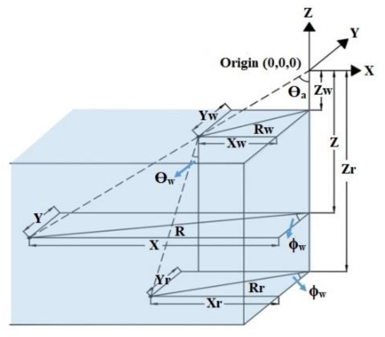
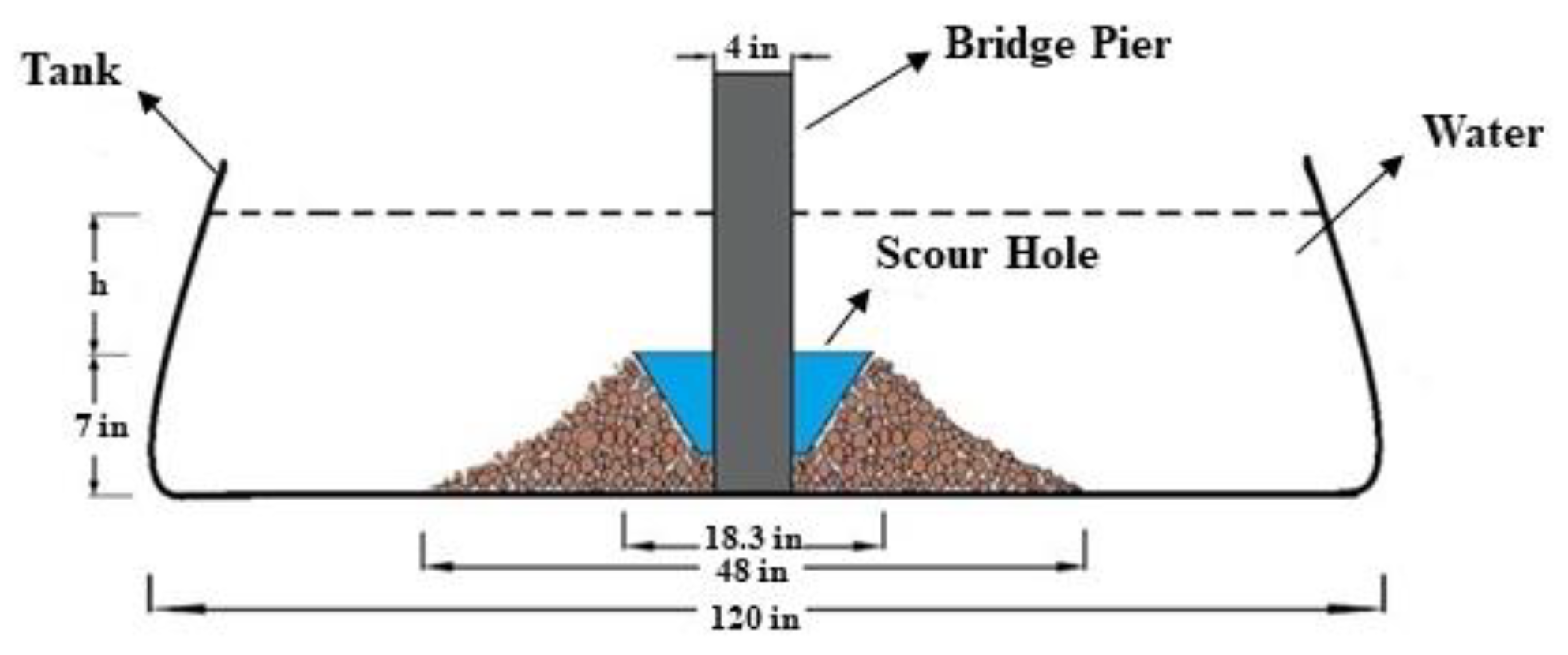
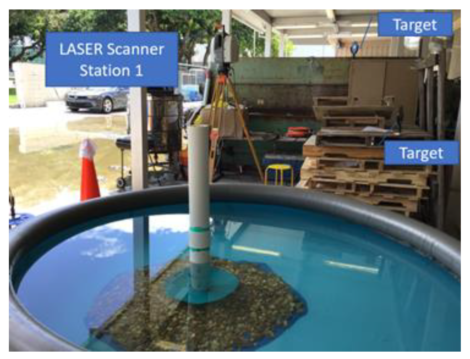
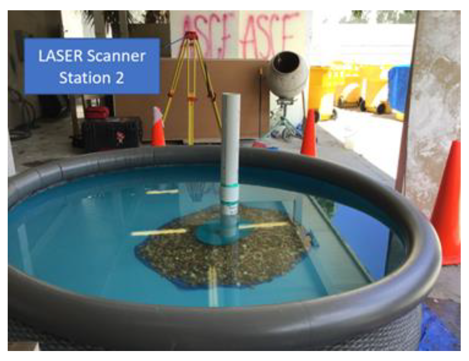
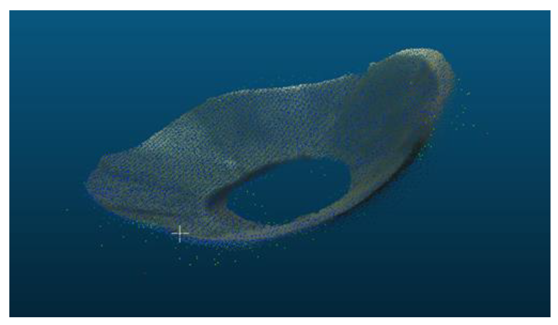
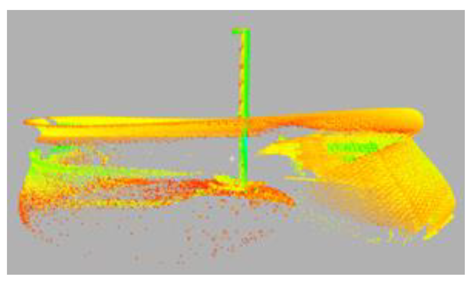
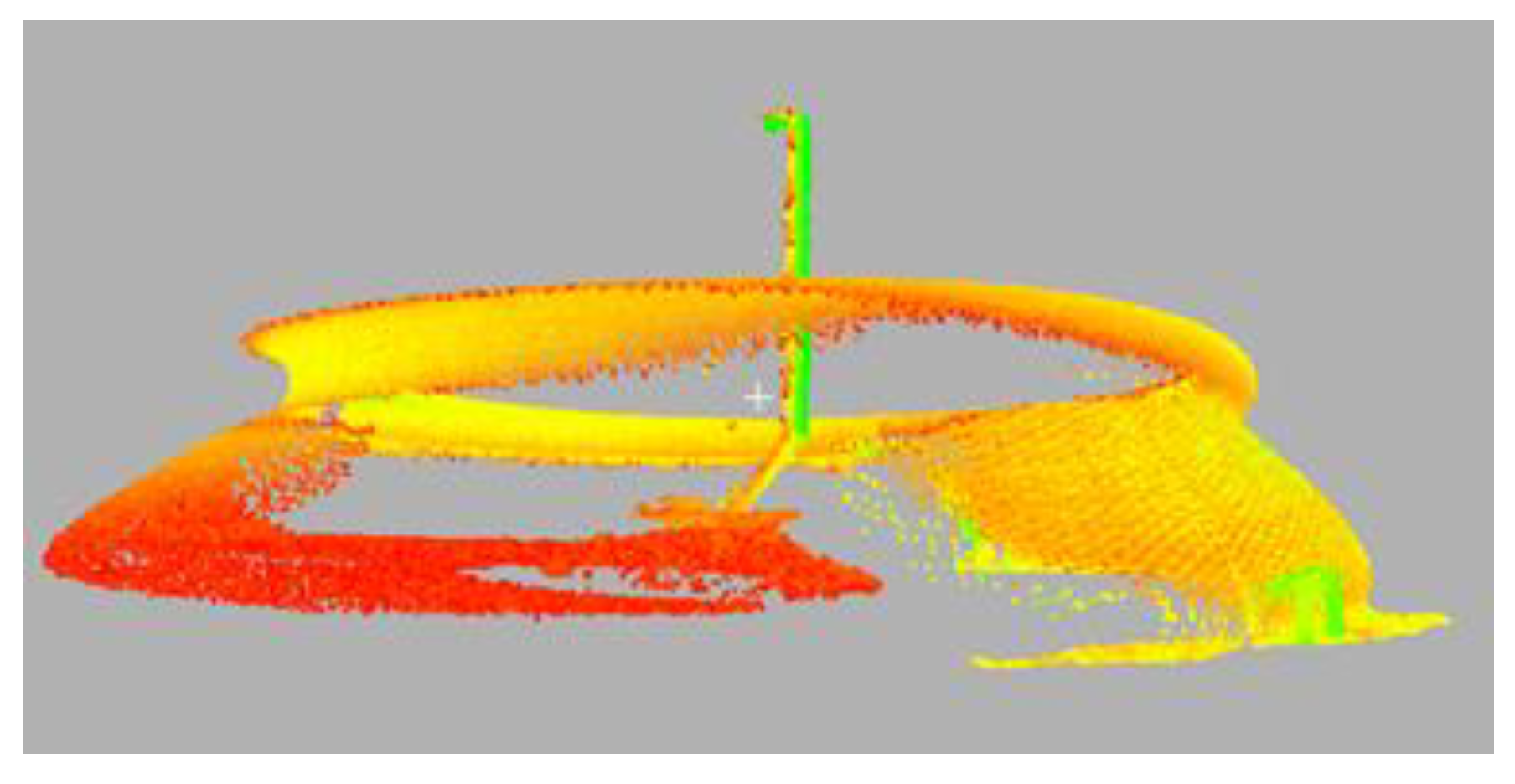
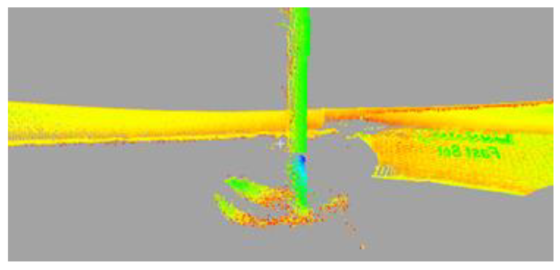
3.1. Experimental Set-Up

The experiment was performed in a 10 ft diameter pool as shown in Figure 1. The maximum allowable water depth of the pool was 30 inches. For the experiment, the water depth was varied from 15 inches to 23.5 inches. Kaolinite powder was used to create the turbidity in the pool. The turbidity of water is defined as the amount of suspended particles which are invisible to the naked eye. The turbidity of the water affects the penetration of the green laser in the water. The algal and non-algal particles, seagrass, mud, silt, microalgae, dissolved organic matter and sand affects the turbidity of water body [33]. The dimensions of the scour hole were taken from earlier published literature of Nagarajan et al., 2018 [31] and Banyhany 2018 [30]. The dimensions of the scour hole were modified for the ease of fabrication. A 4-inch diameter PVC pipe was used as bridge pier which was set at the center of the pool. Leica scan station II was used for the scanning of the scour hole. Trimble X7 (costs $35,000), Surphaser 100HSX (costs $90,000), Leica scan station II (costs $15,000) and FARO Focus S 70 (costs $65,000) are the commonly used terrestrial laser scan devices in the United States. Leica scan station II uses a green laser with a 532 nm wavelength and 4 mm range accuracy. Coarse aggregate was placed along the scour hole with slope of 1: 7.4 to keep the scour hole and bridge pier in place.

Turbidity

The turbidity of the water was measured using an OAKTON T100 turbidity meter by Cole—Parmer. The turbidity of water is measured in Nephelometric Turbidity Units (NTU). According to the United States Geological Survey, the turbidity of river water is usually less than 10 NTU under normal flow conditions. During the time of high floods or heavy rain the turbidity of river can increase over this value [36]. During the time of high floods, the turbidity of river can vary along different locations in a river. The turbidity of water increases as we move towards the river bottom and in the river mouth where there is continuous exchange of water, turbidity can be higher. Before starting the experiment, the turbidity of the clear water was checked, and it was found to be 1.2 NTU. The turbidity was varied from 1.2 NTU to 20.8 NTU by adding Kaolinite. Kaolinite is added gradually to the water in the pool. Water samples from different locations of the pool were collected for measuring the turbidity. The turbidity mentioned throughout in this experimental study is the average turbidity. The results from the scan data shows that the visibility of the scour hole depends on the turbidity of water and water depth. The error in the measured dimensions of the scour hole increases for higher turbidity conditions. From the experimental study it is clear that the underwater scour mapping using a green laser is quite effective in monitoring the underwater scour around bridge pier in turbid waters. The method of underwater scanning can also be used for other areas e.g., detection of underwater objects and bathymetry profiling.

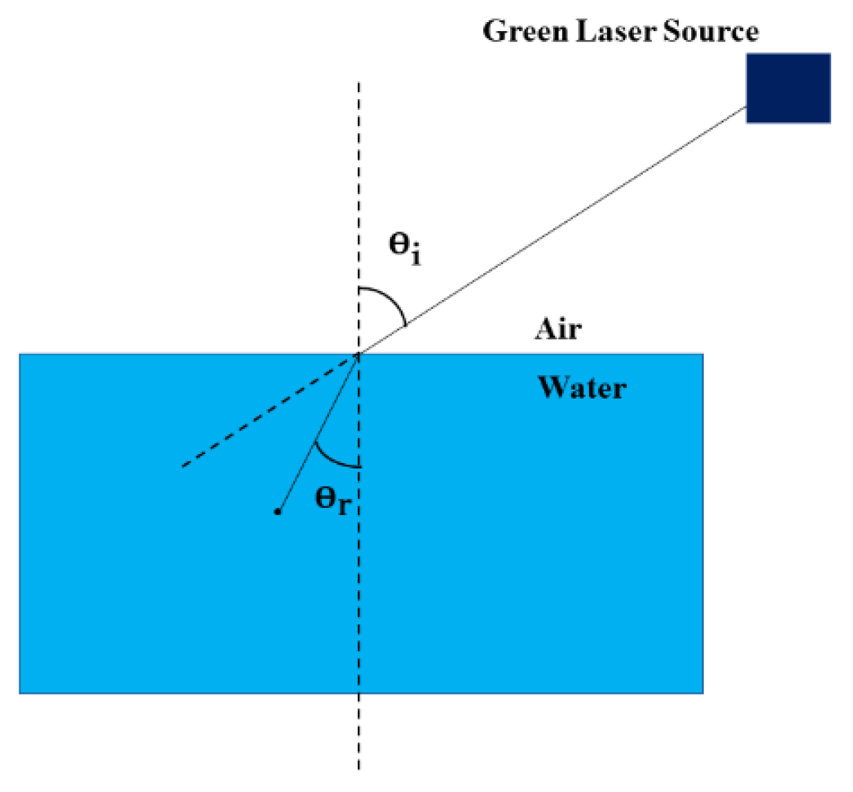
3.2. Refraction Correction Model

The green laser undergoes refraction when it travels from air medium to water medium. The angle of incidence of the green laser with the water medium plays an important role in the amount of refraction. Refraction through the water makes the object look much larger and elevated than its actual position. If the refraction is not considered for underwater scanning, then the error of the underwater submerged topography will be large [37]. This refraction follows Snell’s law. By Snell’s law:
sin   θ i sin   θ r = n 2 n 1
where ϴi—Incident angle, ϴr = refracted angle, n1—Refractive index of air, n2—Refractive index of water. The refractive index depends on the medium of transmission, wavelength of the green laser and temperature [38]. Snell’s law is defined in Cartesian coordinates. For real-life refraction correction, Cartesian coordinates must be converted to polar coordinates. The Cartesian coordinates shown in Figure 2 are converted into Polar coordinates as shown in Figure 3.
The coordinates after refraction correction are shown in Equations (2)–(4) [30,31,38]:
Xr = Rr sin ϕw
Yr = Rr cos ϕw
Z r = 1.33 cos θ w R r R w sin   θ a + Z w
where (Xr, Yr, Zr) are the coordinates after refraction correction, Zw = height of water surface from scanner eyepiece, ϴa = incident angle of laser pulse, ϕw = azimuth of the laser pulse, ϴw = refraction angle.

3.3. Reference Model

Before starting the underwater scanning, the fabricated scour hole was dry scanned to get the dimensions of the scour hole which is used as a reference. The dimensions of the dry scanned scour hole are shown in Figure 4 and Figure 5. The scour hole dimensions from the dry scan are 16.58 inch in width, 14.65 inch in length and 3.10 inch in height. The dry scan was performed to get a reference model which would be used for comparing the results from the underwater scan. The dry scan model will be used as reference model as it is unaffected by turbidity conditions of the water. The absolute error is calculated using the Equation (5):
Absolute error = |Dimensiondry scan − Dimensionfrom trial (with effect of turbidity)|
Absolute error is the modulus of the difference between the dimension measured during the dry scan and the dimension measured during the trials with the effect of turbidity.

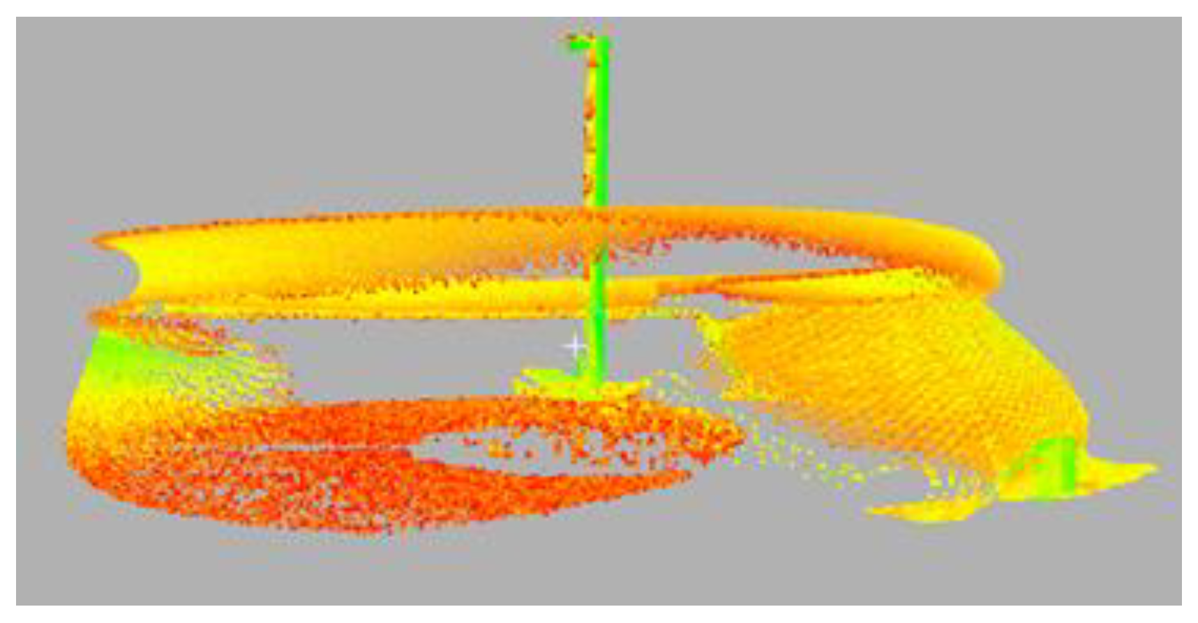
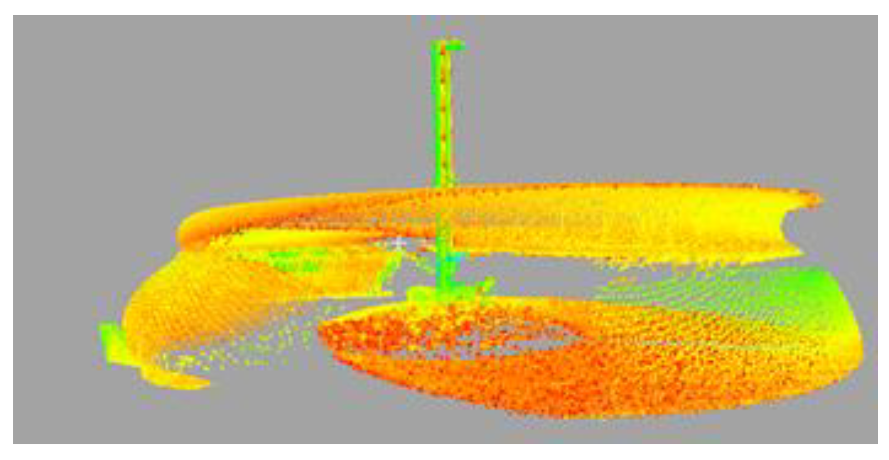
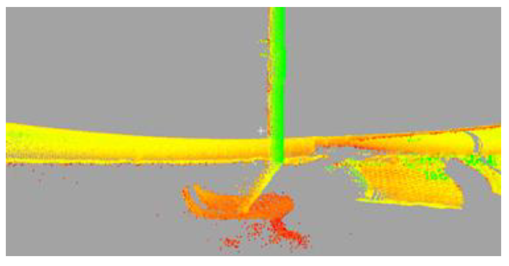
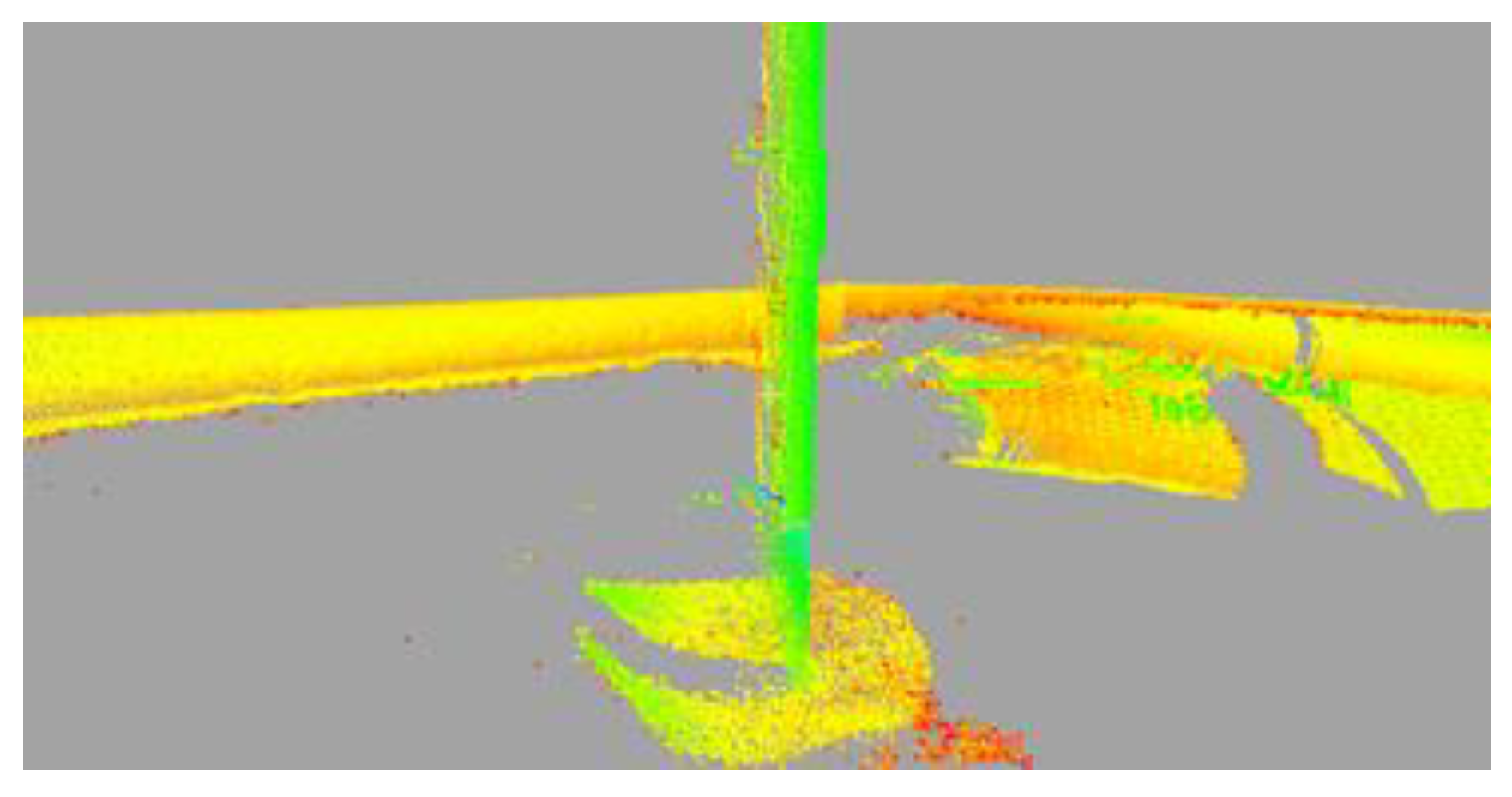
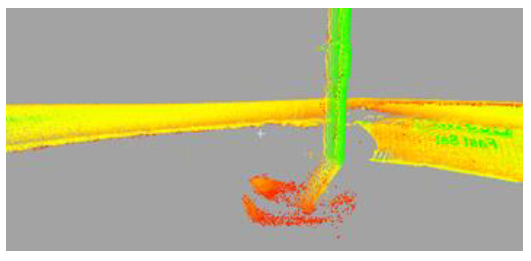
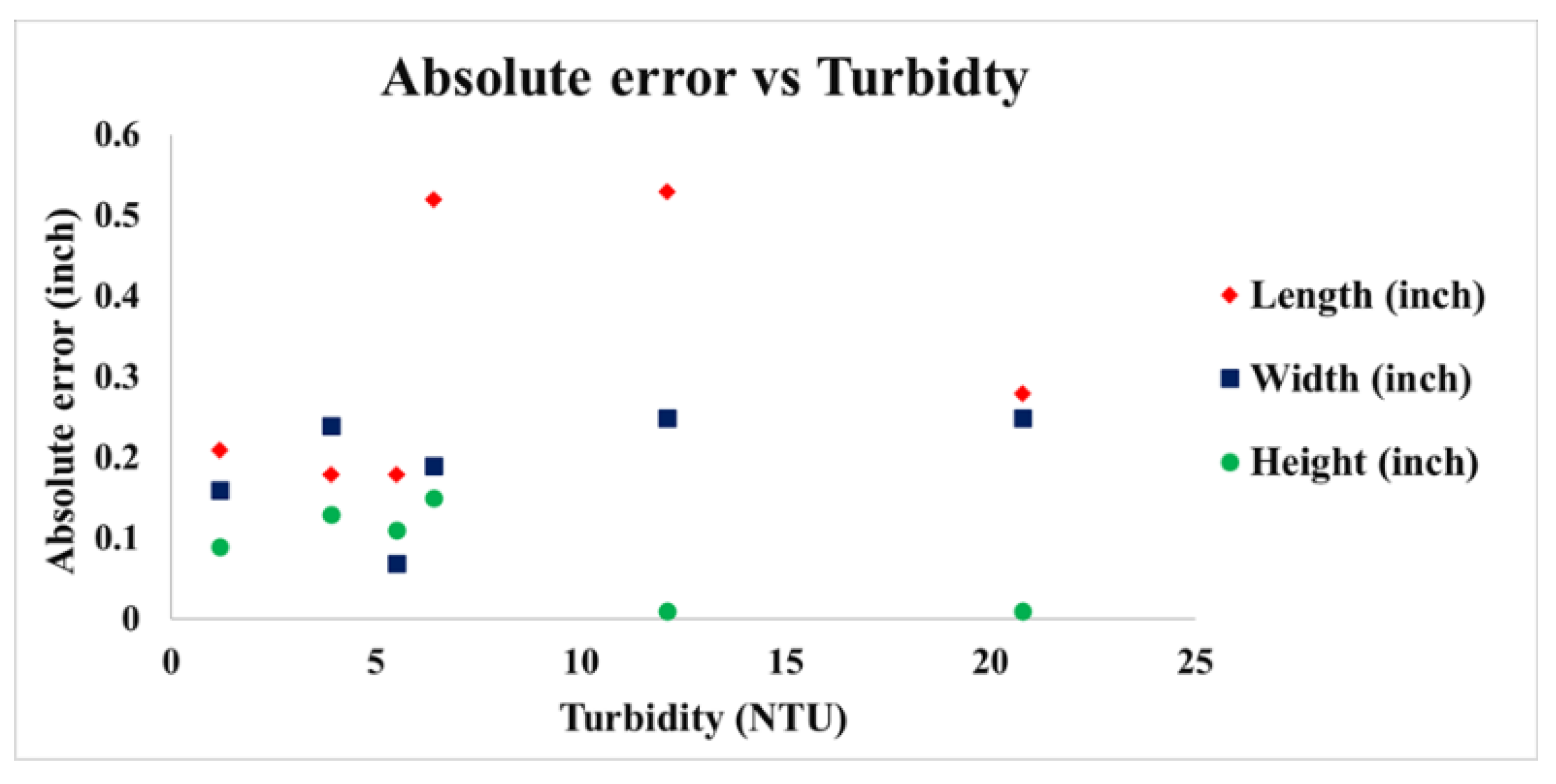
4. Results and Discussion

The penetration depth of the green laser depends on the type and power of the green laser, relative Secchi depth and the turbidity of the water [39]. To get full 360° view of the scour hole, two scan stations are set up as shown in Figure 6 and Figure 7. The six set of trials were conducted at these two stations. The parameters considered here during the underwater scanning are point density, reflectance, minimum range, and maximum range. For the experiments, the point spacing considered is 5 mm at 15 feet range. 1% reflectance of incident energy is also considered here for the scanning. Once the pool is setup with a fabricated scour hole and pier, the tripod with laser scanner is levelled and connected to cyclone software for data collection. A total of five targets were used to record (merge) the three-dimensional laser scan data collected from the two stations. Two out of the five targets are visible in Figure 6. All the five targets used for registration were visible from both the stations.

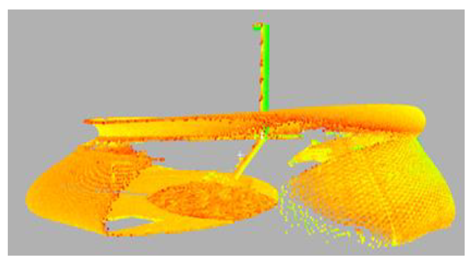
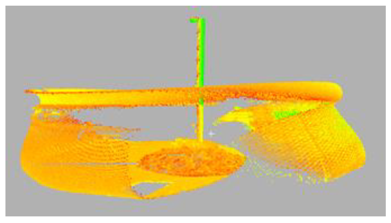
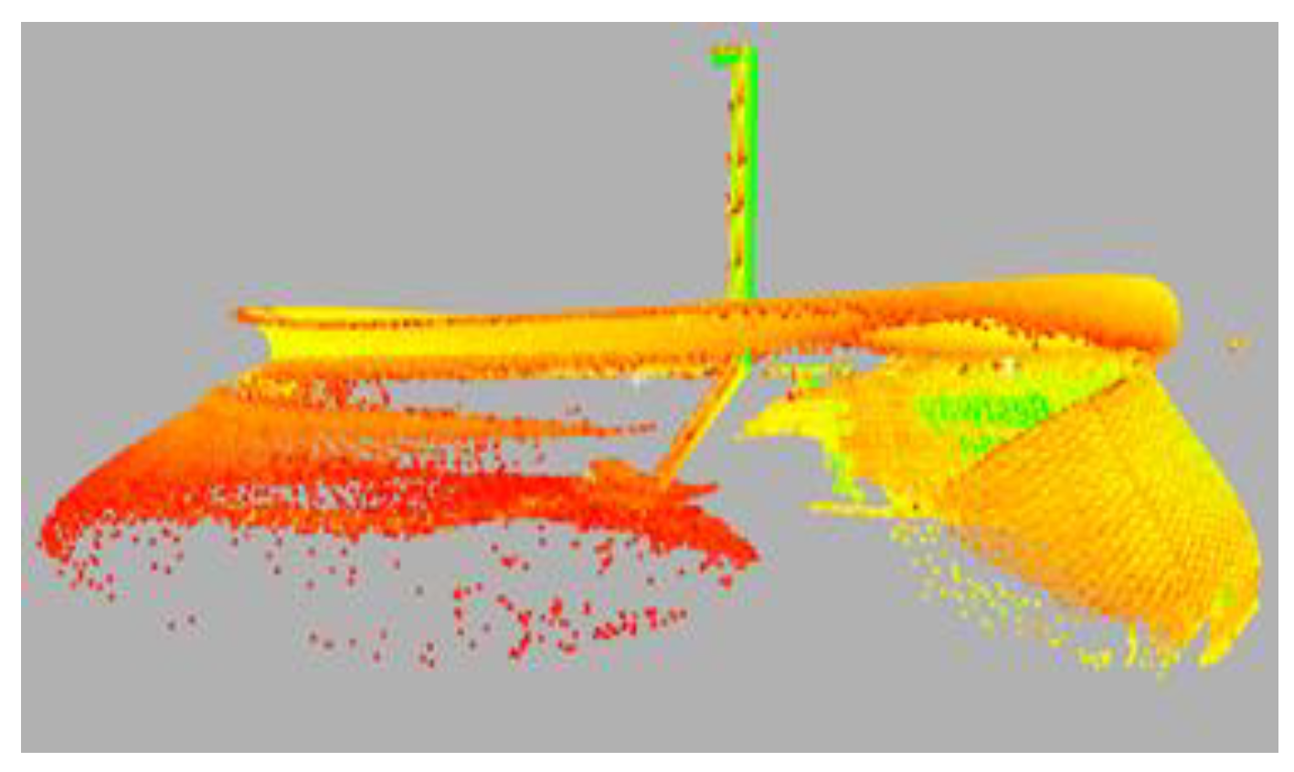
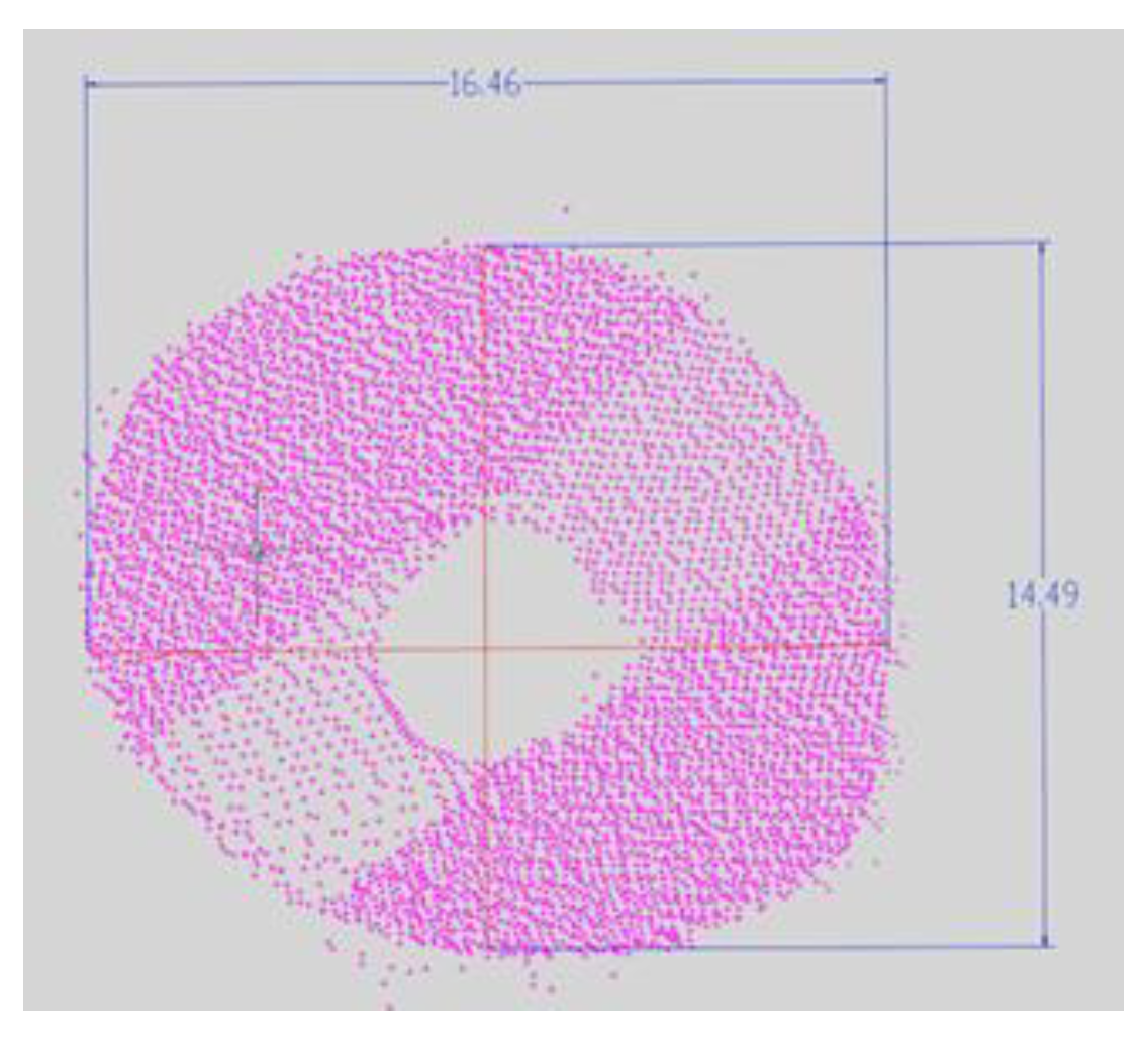
4.1. Turbidity 1.2 NTU (Trial 1)

After the dry scan, the initial scanning was conducted for clear water condition. The turbidity of clear water was found to be 1.2 NTU. The water depth measured around the fabricated scour hole was 16.5 inch. The water depth measured elsewhere in the tank was 20.5 inch. The scour hole was scanned from the two stations for target registration. The refraction correction is applied to the scan data and the data is registered using target to target registration method. The target-to-target registration method uses common targets. These targets are visible from both the stations. Figure 8 and Figure 9 show the 3D scan of the setup before and after applying the refraction rectifications for Trial 1. Figure 10 and Figure 11 show the measurements of the scour hole after applying the refraction rectifications for Trial 1. The scour hole dimensions from Trial 1 are 16.46 inch in width, 14.49 inch in length and 3.01 inch in height.
For Trial 1, the absolute error in width is 0.12 inch, 0.16 inch in length and 0.09 inch in height.

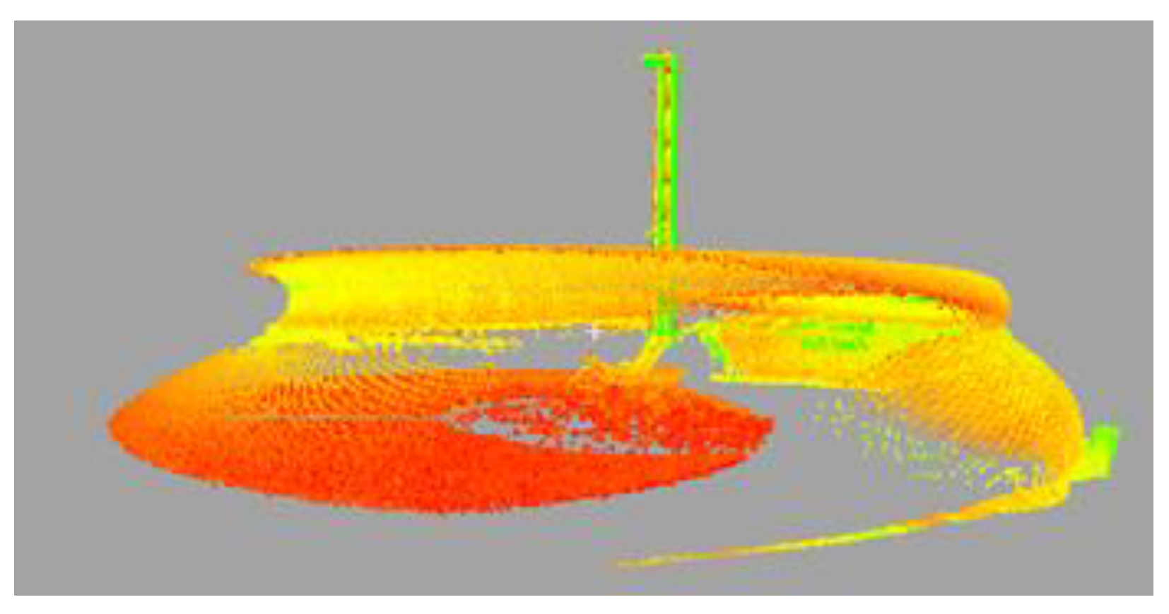
4.2. Turbidity 3.9 NTU (Trial 2)

During the second trial, Kaolinite powder was mixed to the clear water to increase the turbidity. After adding the Kaolinite powder, the turbidity of the water was checked. The turbidity of water was measured as 3.9 NTU. The turbidity of the water in the pool increased after the addition of Kaolinite powder. The water depth near the scour hole was 16.5 inch and it was 20.5 inch elsewhere in the pool. The advantage of using Kaolinite powder is that it easily suspends in the water rather than floating on the water surface or settling in the bottom of the water. The average size of the Kaolinite powder particle is 1.5-micron which makes it easy to suspend in the water.
Figure 12 and Figure 13 show the 3D scan of the setup before and after refraction correction for Trial 2. For Trial 2 the scour hole was completely visible during the scanning using the green laser. The dimensions of the scour hole from Trial 2 are 16.4 inch in width, 14.41 inch in length and 2.97 inch in height. The absolute error in length is 0.24 inch, in width is 0.18 inch and in height is 0.13 inch. The absolute error got increased for Trial 2 compared to Trial 1. This is due to the fact that the reflected rays from the scour hole get reduced due to increase in the turbidity of the water. Some of the rays get scattered and do not get reflected back to the laser scanner.

4.3. Turbidity 5.5 NTU (Trial 3)

The turbidity of the water in the pool was increased by adding more Kaolinite powder to the water. The water in the pool became milky which was a clear indication of the increase in the turbidity. While scanning the setup with the increased turbidity, the sour hole was not visible. This indicates that with the increase in turbidity the ability of the laser to penetrate the water also gets reduced. So, the water level in the pool was reduced and the scanning process was continued. The scour hole was clearly visible from the scanned data. The water depth near the scour hole was around 12.5 inch and elsewhere in the pool it was 16.5 inch. Figure 14 and Figure 15 show the three-dimensional scan of the setup before and after the refraction correction for Trial 3. The dimensions of the scour hole from the scan were 14.72 inch in length, 16.4 inch in width and 2.99 inch in height. The absolute error in length was 0.07 inch, 0.18 inch in width and 0.11 inch in height.

4.4. Turbidity 6.4 NTU (Trial 4)

In Trial 4 more Kaolinite powder was added to the prevailing Trial 3 conditions. The turbidity was measured, and it was found to be 6.4 NTU. Figure 16 and Figure 17 show the three-dimensional scan of the setup before and after applying the refraction correction for Trial 4. The dimensions of the scour hole from the scan were 17.1 inch in width, 14.46 inch in length and 2.95 inch in height. The absolute error in length was 0.19 inch, 0.52 inch in width and 0.15 inch in height. The laser scanner was able to see the bed topography until turbidity 6.4 NTU. The water depth near the scour hole was 12.5 inch. The water depth in other areas was 16.5 inch. The absolute error was increased for Trial 4 compared earlier trials. This is because the reflected rays from the scour hole become reduced due to increase in the turbidity of the water. Some of the rays get scattered and do not get reflected back to the laser scanner.

4.5. Turbidity 12.1 NTU (Trial 5)

Turbidity was increased by adding Kaolinite powder to the existing condition. The turbidity was increased to 12.1 NTU. The green laser was not able to see the scour hole and bed topography. The turbidity of the water influences the passing of the green laser through the water [33]. The water depth near the scour hole was reduced to 8 inches. This also indicates that with the increase in turbidity the ability of the laser to penetrate the water also gets reduced. In other areas of pool bed, the water depth was 12 inches. Even after reducing the water level, the bed topography was not visible. The scour hole was fully visible. Figure 18 and Figure 19 show the three-dimensional scan of the setup before and after applying the refraction correction for Trial 5. The dimensions of the scour hole from the scan results were 17.11 inch in width, 14.4 inch in length and 3.09 inch in height. The bed topography was visible until turbidity 6.4 NTU. After increasing the turbidity from 6.4 NTU to 12.1 NTU, the bed topography was not visible, only the scour hole was visible. The absolute error in length was 0.25 inch, 0.53 inch in width and 0.01 inch in height.

4.6. Turbidity 20.8 NTU (Trial 6)

The turbidity was increased from 12.1 NTU to 20.8 NTU by adding more Kaolinite powder keeping the same water depth as of Trial 5. Figure 20 and Figure 21 show the three-dimensional scan of the setup before and after applying the refraction correction for Trial 6. The measurements of the scour hole from the laser scan were 14.4 inch in length, 16.3 inch in width and 3.09 inch in height. The absolute error with respect to dry scan in length was 0.25 inch, in width was 0.28 inch and in height was 0.01 inch. From the scan results the green laser was able to capture the scour hole only; the bed topography was not visible. The scour hole was not completely visible as for the earlier cases. From the scan results the bed topography was not visible, and the scour hole was not completely visible.
The summary of the results of the experiments is shown in Table 1. The variation in absolute error with respect to the dry scan model for width, length, and height of the scan results with turbidity is shown in Figure 22. The absolute error in length is showing an increasing trend except for Trials 3 and 4 which can be due to the errors encountered during the experiment. The absolute error for width increases with increase in turbidity until Trial 5. The absolute error for height is showing an increasing trend except for Trial 3, 5 and 6. For Trial 3, 5 and 6 the absolute error in height is showing a decrease which can be due to errors encountered while performing the experiment. For Trial 6 the absolute error in width shows deviation from the general increasing trend and it is suddenly decreasing. The graph shows the restriction of the green laser to record the sharp corners of the scour hole which is a limitation in extracting the exact dimensions of the scour hole [32].

5. Conclusions

The method of underwater scanning using a green laser for detecting scour around bridge pier is safe, efficient, and economical. Six set of trials were conducted in the pool with pier and fabricated scour hole. Initially the experiment was carried out in clear water of turbidity 1.2 NTU. More trials were conducted for turbidity of 3.9 NTU, 5.5 NTU, 6.4 NTU, 12.1 NTU and 20.8 NTU by adding Kaolinite powder to the clear water. During low turbidity levels the scour hole and bed topography were visible in the laser scanning. For higher turbidity levels the edges of the scour hole were not properly visible. The bed topography and scour hole were clearly visible for turbidity values less than 6.4 NTU. The error in the measured dimensions of the scour hole also increased for higher turbidities. The ability of the green laser to capture the fabricated scour hole and pool bed topography decreased as the turbidity was increased even when the water depth was reduced. The absolute error in length is showing an increasing trend except for Trials 3 and 4 which can be due to the errors encountered during the experiment. The absolute error for height is showing an increasing trend except for Trials 3, 5 and 6. For Trials 3, 5 and 6 the absolute error in height is showing a decrease which can be due to errors encountered while performing the experiment. The absolute error for width increases with increase in turbidity until Trial 5. For Trial 6 the absolute error in width shows a deviation from the general increasing trend and it is suddenly decreasing.
The sharp edges of the scour hole were not able to see as the turbidity was increased [32]. In actual field conditions the scour hole profile dimensions will not be having sharp edges as seen in the fabricated scour hole here in the experiments. The depth of penetration of the green laser depends on the water turbidity, laser range, type and power of the green laser and laser inclination angle [32,40]. Here the green laser was able to penetrate to a depth of 2 ft inside the pool under turbid conditions. The Root Mean Square (RMS) errors from the six trials of experiments are 0.34 inch in width, 0.20 inch in length and 0.1 inch in depth. So, the method of using a green laser for underwater scanning is effective and can also be used in other areas, such as bathymetry profiling and detection of underwater objects. Further studies can be conducted by integrating a green laser to drones for the scanning of scour around the pier and bathymetry profiling.

6. Field Testing

The method discussed here, measuring scouring around the bridge pier was used to check the scour around a railroad bridge located in Miami-Dade County, Florida and a highway bridge located in the Little Lake Worth, Florida.

Author Contributions

Conceptualization, R.D.R., S.N., M.A. and S.C.; methodology, R.D.R., S.N., M.A. and S.C.; software, S.N., S.C. and R.D.R.; validation, S.N., S.C. and R.D.R.; formal analysis, R.D.R., S.N. and S.C.; investigation, R.D.R., S.N., M.A. and S.C.; resources, R.D.R., S.N., M.A. and S.C.; data curation, R.D.R., S.N. and S.C.; writing—Original draft preparation, R.D.R.; writing—Review and editing, R.D.R. and S.N.; visualization, S.N.; supervision, S.N. and M.A.; project administration, S.N.; funding acquisition, S.N. All authors have read and agreed to the published version of the manuscript.

Funding

This project was funded by the National Academies of Sciences, Engineering & Medicine, USA, grant number—SAFETY-39, and Transportation Research Board’s Rail Safety IDEA Program, USA, grant number—BDV27-977-16.

Institutional Review Board Statement

Not applicable.

Informed Consent Statement

Not applicable.

Data Availability Statement

Not applicable.

Acknowledgments

The authors would like to thank CSX Transportation and Florida Department of Transportation for their support. Authors would like to thank Florida Department of Transportation (FDOT), USA and Transportation Research Board (TRB), USA for giving permission to use data from the reports of project for this paper.

Conflicts of Interest

The authors declare no conflict of interest. The funders had no role in the design of the study; in the collection, analyses, interpretation of data; or in the writing of the manuscript. The funders gave consent to publish data from the reports of project.

References

  1. Browne, T.M.; Collins, T.J.; Garlich, M.J.; O’Leary, J.E.; Stromberg, D.G.; Heringhaus, K.C. Underwater Bridge Inspection (No. FHWA-NHI-10-027); Federal Highway Administration, Office of Bridge Technology: Washington, DC, USA, 2010.
  2. Wardhana, K.; Hadipriono, F.C. Analysis of recent bridge failures in the United States. J. Perform. Constr. Facil. 2003, 17, 144–150. [Google Scholar]
  3. Arneson, L.A.; Zevenbergen, L.W.; Lagasse, P.F.; Clopper, P.E. Evaluating Scour at Bridges (No. FHWA-HIF-12-003); National Highway Institute (US), Repository and Open Science Access Portal, Naional Transportation Library: Washington, DC, USA, 2012.
  4. Lamb, R.; Garside, P.; Pant, R.; Hall, J.W. A probabilistic model of the economic risk to Britain’s railway network from bridge scour during floods. Risk Anal. 2019, 39, 2457–2478. [Google Scholar]
  5. Benedict, S.T.; Caldwell, A.W. A Pier-Scour Database: 2427 Field and Laboratory Measurements of Pier Scour; 845; U.S. Geological Survey: Reston, VA, USA, 2014. [CrossRef]
  6. Hearn, G. Bridge Inspection Practices (Vol. 375); Transportation Research Board: Washington, DC, USA, 2007. [Google Scholar]
  7. Deng, L.; Wang, W.; Yu, Y. State-of-the-art review on the causes and mechanisms of bridge collapse. J. Perform. Constr. Facil. 2016, 30, 04015005. [Google Scholar]
  8. Lagasse, P.F.; Richardson, E.V. ASCE compendium of stream stability and bridge scour papers. J. Hydraul. Eng. 2011, 127, 531–533. [Google Scholar]
  9. Lu, J.Y.; Hong, J.H.; Su, C.C.; Wang, C.Y.; Lai, J.S. Field measurements and simulation of bridge scour depth variations during floods. J. Hydraul. Eng. 2008, 134, 810–821. [Google Scholar]
  10. Prendergast, L.J.; Gavin, K. A review of bridge scour monitoring techniques. J. Rock Mech. Geotech. Eng. 2014, 6, 138–149. [Google Scholar]
  11. Kobayashi, T.; Oda, K. Experimental study on developing process of local scour around a vertical cylinder. In Coastal Engineering, Proceedings of Twenty-Fourth International Conference, Kobe, Japan, 23–28 October 1994; ASCE: Columbia, MD, USA; pp. 1284–1297.
  12. Anderson, N.L.; Ismael, A.M.; Thitimakorn, T. Ground-penetrating radar: A tool for monitoring bridge scour. Environ. Eng. Geosci. 2007, 13, 1–10. [Google Scholar]
  13. Yao, C.; Darby, C.; Hurlebaus, S.; Price, G.R.; Sharma, H.; Hunt, B.E.; Yu, O.-Y.; Chang, K.-A.; Briaud, J.-L. Scour monitoring development for two bridges in Texas. Proceedings 5th International Conference on Scour and Erosion (ICSE-5), San Francisco, CA, USA, 7–10 November 2010; pp. 958–967. [Google Scholar]
  14. Whitehouse, R.J.; Sutherland, J.; Harris, J.M. Evaluating scour at marine gravity foundations. In Proceedings of the Institution of Civil Engineers-Maritime Engineering; Thomas Telford Ltd.: London, UK, 2011; Volume 164, pp. 143–157. [Google Scholar]
  15. Lin, Y.B.; Chen, J.C.; Chang, K.C.; Chern, J.C.; Lai, J.S. Real-time monitoring of local scour by using fiber Bragg grating sensors. Smart Mater. Struct. 2005, 14, 664. [Google Scholar]
  16. Kong, X.; Ho, S.C.M.; Song, G.; Cai, C.S. Scour monitoring system using fiber Bragg grating sensors and water-swellable polymers. J. Bridge Eng. 2017, 22, 04017029. [Google Scholar]
  17. Prendergast, L.J. Monitoring of bridge scour using changes in natural frequency of vibration-a field investigation. In Proceedings of the 5th International Young Geotechnical Engineer’s Conference, Paris, France, 31 August–1 September 2013; IOS Press: Amsterdam, The Netherland, 2013. [Google Scholar]
  18. Fisher, M.; Atamturktur, S.; Khan, A.A. A novel vibration-based monitoring technique for bridge pier and abutment scour. Struct. Health Monit. 2013, 12, 114–125. [Google Scholar]
  19. Lagasse, P.F.; Richardson, E.V.; Schall, J.D. Fixed instrumentation for monitoring scour at bridges. Transp. Res. Rec. 1998, 1647, 1–9. [Google Scholar]
  20. Deng, L.; Cai, C.S. Bridge scour: Prediction, modeling, monitoring, and countermeasures. Pract. Period. Struct. Des. Constr. 2010, 15, 125–134. [Google Scholar]
  21. Schall, J.D. Sonar Scour Monitor: Installation, Operation, and Fabrication Manual; Transportation Research Board, National Academy Press: Washington, DC, USA, 1997. [Google Scholar]
  22. Fisher, M.; Chowdhury, M.N.; Khan, A.A.; Atamturktur, S. An evaluation of scour measurement devices. Flow Meas. Instrum. 2013, 33, 55–67. [Google Scholar]
  23. Webb, D.J.; Anderson, N.L.; Newton, T.; Cardimona, S. Bridge scour: Application of ground penetrating radar. In Proceedings of the First International Conference on the Application of Geophysical Methodologies and NDT to Transportation Facilities and Infrastructure, St. Louis, MO, USA, 11–15 December 2000; Federal Highway Commission and Missouri Department of Transportation: St. Louis, MO, USA, 2000. [Google Scholar]
  24. Park, I.; Lee, J.; Cho, W. Assessment of bridge scour and riverbed variation by a ground penetrating radar. In Proceedings of the Tenth International Conference on Grounds Penetrating Radar, GPR 2004, Delft, The Netherland, 21–24 June 2004; IEEE: Piscataway, NJ, USA, 2004; Volume 1, pp. 411–414. [Google Scholar]
  25. Placzek, G. Surface-Geophysical Techniques Used to Detect Existing and Infilled Scour Holes Near Bridge Piers; US Department of the Interior, US Geological Survey: Hartford, CT, USA, 1995; Volume 95.
  26. Porter, K.; Simons, R.; Harris, J. Comparison of three techniques for scour depth measurement: Photogrammetry, echosounder profiling and a calibrated pile. Coast. Eng. Proc. 2014, 34, 64. [Google Scholar]
  27. Lasa, I.R.; Hayes, G.H.; Parker, E.T. Remote Monitoring of Bridge Scour Using Echo Sounding Technology. In Transportation Research Circular 498; Proceedings of the Presentations from 8th International Bridge Management Conference, Denver, CO, USA, 26–28 April 1999; Transportation Research Board: Washington, DC, USA, 2000; Volume 1. [Google Scholar]
  28. Mueller, D.S.; Landers, M.N. Portable Instrumentation for Real-Time Measurement of Scour at Bridges (No. FHWA-RD-99-085); Federal Highway Administration, Repository and Open Science Access Portal, Naional Transportation Library: Washington, DC, USA, 2000.
  29. Yagci, O.; Yildirim, I.; Celik, M.F.; Kitsikoudis, V.; Duran, Z.; Kirca, V.O. Clear water scour around a finite array of cylinders. Appl. Ocean Res. 2017, 68, 114–129. [Google Scholar]
  30. Banyhany, M. 3D Reconstruction of Simulated Bridge Pier Local Scour Using Green Laser and Hydrolite Sonar. Master’s Thesis, Florida Atlantic University, Boca Raton, FL, USA, 2018. [Google Scholar]
  31. Nagarajan, S.; Arockiasamy, M.; Banyhany, M. Bridge Pier Scour Hole Simulation and 3D Reconstruction Using Green Laser (No. 18-05495). In Proceedings of the Compendium of Transportation Research Board 97th Annual Meeting, Washington DC, USA, 7–11 January 2018. [Google Scholar]
  32. Paul, J.D.; Buytaert, W.; Sah, N. A Technical Evaluation of Lidar-Based Measurement of River Water Levels. Water Resour. Res. 2020, 56, e2019WR026810. [Google Scholar]
  33. Brando, V.E.; Anstee, J.M.; Wettle, M.; Dekker, A.G.; Phinn, S.R.; Roelfsema, C. A physics based retrieval and quality assessment of bathymetry from suboptimal hyperspectral data. Remote Sens. Environ. 2009, 113, 755–770. [Google Scholar]
  34. Fabricius, K.E.; De’ath, G.; Humphrey, C.; Zagorskis, I.; Schaffelke, B. Intra-annual variation in turbidity in response to terrestrial runoff on near-shore coral reefs of the Great Barrier Reef. Estuarine. Coast. Shelf Sci. 2013, 116, 57–65. [Google Scholar]
  35. Nagarajan, S.; Arockiasamy, M. Non-Contact Scour Monitoring System for Railroad Bridges (No. Rail Safety IDEA Project 39); Transportation Research Board: Washington, DC, USA, 2020. [Google Scholar]
  36. Nagarajan, S.; Arockiasamy, M. Non-Contact Scour Monitoring for Highway Bridges; Repository and Open Science Access Portal, Naional Transportation Library: Washington, DC, USA, 2020.
  37. Milan, D.J.; Heritage, G.L.; Hetherington, D. Application of a 3D laser scanner in the assessment of erosion and deposition volumes and channel change in a proglacial river. Earth Surf. Processes Landf. J. Br. Geomorphol. Res. Group 2007, 32, 1657–1674. [Google Scholar]
  38. Smith, M.; Vericat, D.; Gibbins, C. Through-water terrestrial laser scanning of gravel beds at the patch scale. Earth Surf. Processes Landf. 2012, 37, 411–421. [Google Scholar]
  39. Zhao, J.; Zhao, X.; Zhang, H.; Zhou, F. Shallow water measurements using a single green laser corrected by building a near water surface penetration model. Remote Sens. 2017, 9, 426. [Google Scholar]
  40. Guenther, G.C.; Cunningham, A.G.; LaRocque, P.E.; Reid, D.J. Meeting the Accuracy Challenge in Airborne Bathymetry; National Oceanic Atmospheric Administration/Nesdis Silver Md.: Silver Spring, MD, USA, 2000.
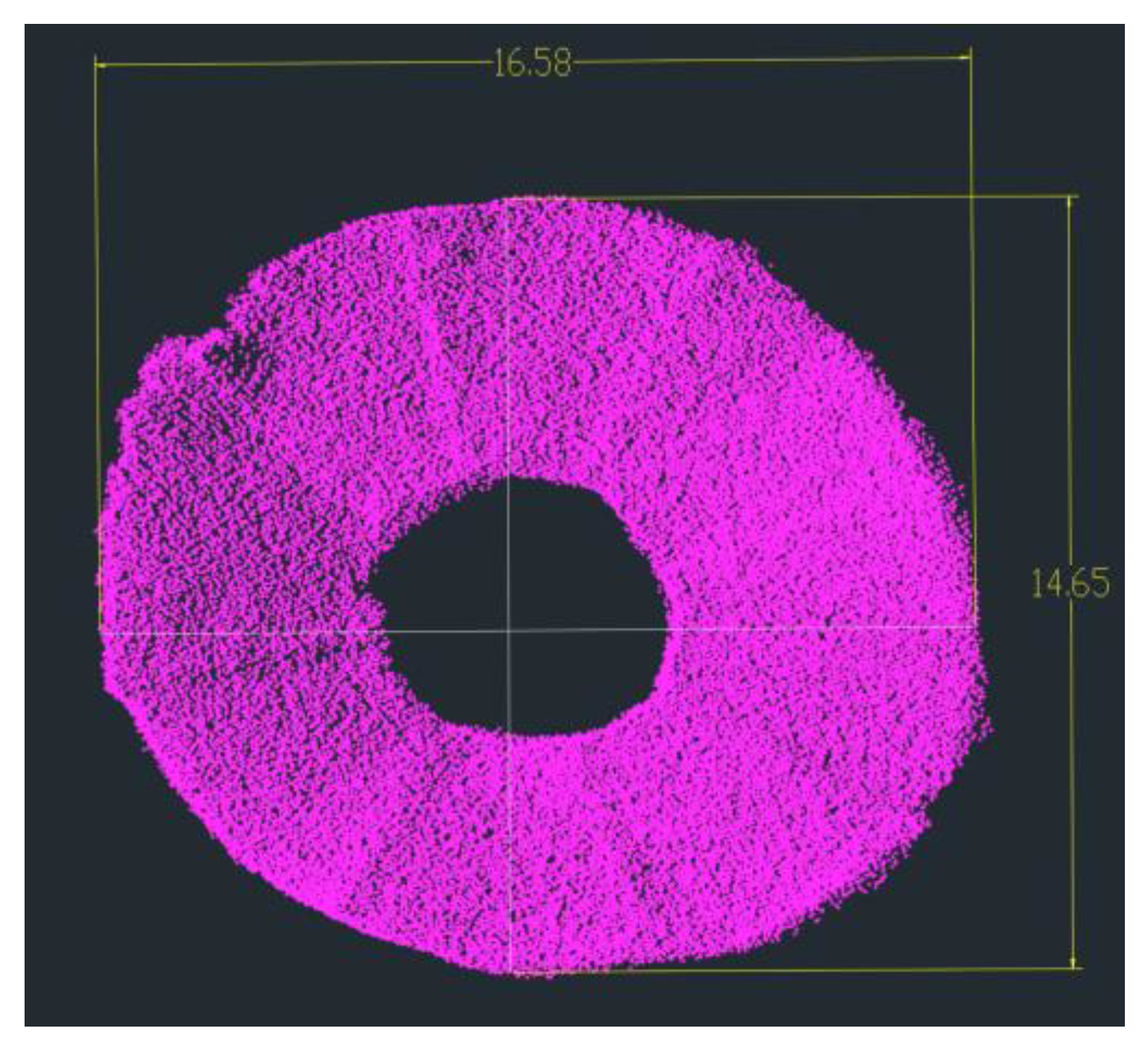
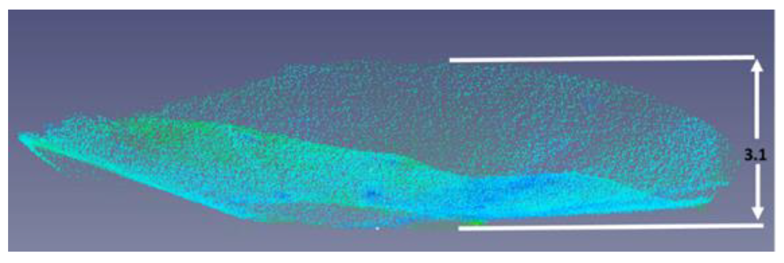
Figure 1. Schematic diagram of experimental set-up [34,35] (used with permission).
Geomatics 02 00020 g001
Figure 2. Schematic diagram of refraction of a green laser in water.
Geomatics 02 00020 g002
Figure 3. Schematic diagram of refraction correction applied for underwater scanning inside the 10 ft diameter pool [adapted from Smith et al.] [31,38].
Geomatics 02 00020 g003
Figure 4. Schematic Dimensions of scour hole in dry scan (all units are in inches) [35,36] (used with permission).
Geomatics 02 00020 g004
Figure 5. Depth of sour hole in dry scan (depth is in inch) [35,36] (used with permission).
Geomatics 02 00020 g005
Figure 6. Scan station one in operation [35,36] (used with permission).
Geomatics 02 00020 g006
Figure 7. Scan station two in operation [35,36] (used with permission).
Geomatics 02 00020 g007
Figure 8. 3D laser scan before refraction correction for Trial 1 [35,36] (used with permission).
Geomatics 02 00020 g008
Figure 9. 3D laser scan after refraction correction for Trial 1 [35,36] (used with permission).
Geomatics 02 00020 g009
Figure 10. Dimensions of retrieved scour model for Trial 1 (all units are in inches) [35,36] (used with permission).
Geomatics 02 00020 g010
Figure 11. 3D overlay of retrieved scour model for Trial 1 [35,36] (used with permission).
Geomatics 02 00020 g011
Figure 12. 3D laser scan before refraction correction for Trial 2 [35,36] (used with permission).
Geomatics 02 00020 g012
Figure 13. 3D laser scan after refraction correction for Trial 2 [35,36] (used with permission).
Geomatics 02 00020 g013
Figure 14. 3D laser scan before refraction correction for Trial 3 [35,36] (used with permission).
Geomatics 02 00020 g014
Figure 15. 3D laser scan after refraction correction for Trial 3 [35,36] (used with permission).
Geomatics 02 00020 g015
Figure 16. Three-dimensional laser scan before refraction correction for Trial 4 [36] (used with permission).
Geomatics 02 00020 g016
Figure 17. Three-dimensional laser scan after refraction correction for Trial 4 [36] (used with permission).
Geomatics 02 00020 g017
Figure 18. Three-dimensional laser scan before refraction correction for Trial 5 [36] (used with permission).
Geomatics 02 00020 g018
Figure 19. Three-dimensional laser scan after refraction correction for Trial 5 [36] (used with permission).
Geomatics 02 00020 g019
Figure 20. Three-dimensional laser scan before refraction correction for Trial 6 [36] (used with permission).
Geomatics 02 00020 g020
Figure 21. Three-dimensional laser scan after refraction correction for Trial 6 [36] (used with permission).
Geomatics 02 00020 g021
Figure 22. Effect of turbidity on the absolute error (adapted from Nagarajan & Arockiasamy, 2020a and 2020b) [35,36].
Geomatics 02 00020 g022
Table 1. Summary of results from the experiment [35,36] (used with permission).
Trial No.Turbidity (NTU)Water Depth Near the Scour Hole (Inches)Water Depth in Other Parts of the Pool (Inches)Measured Scour Hole Dimensions
Length (Inches)Width (Inches)Height (Inches)
11.216.520.514.4916.463.01
23.916.520.514.4116.42.97
35.512.516.514.7216.42.99
46.412.516.514.4617.12.95
512.181214.417.113.09
620.881214.416.33.09
Publisher’s Note: MDPI stays neutral with regard to jurisdictional claims in published maps and institutional affiliations.

