Abstract
The single polarization C-Band weather radar network of the Meteorological Service of Catalonia covers the entire region (32,000 km2), which allows it to apply a series of corrections that improve preliminary estimations of the rainfall field (hourly and daily). In addition, an automatic re-processing using automatic weather stations helps to incorporate ground-based information. The last process of the quantitative precipitation estimation (QPE) is running the end-product again eight days later, when the data have been reviewed and corrected in the case of detecting anomalies in the radar or gauge data. These corrections are applied operationally, with the fields generated and stored automatically. The QPE fields are generated in the GeoTIFF format, allowing easy use with multiple applications and simplifying processes such as quality control. In this way, the analysis of a 10 year period of GeoTIFF QPE daily data compared with ground rainfall values is introduced. The results help to understand different points regarding the functioning of the network such as the dependance on the type of precipitation and the seasonality. In addition, the description of a heavy rainfall episode (22 October 2019) shows the variations and improvements in the different products. The main conclusions refer to how using GeoTIFF combined with point data (rain gauges), it is possible to ensure simple but effective quality control of an operational radar network.
Keywords:
QPE; weather radar; bias; rain gauges; corrections; heavy rainfall; quality control; GeoTIFF 1. Introduction
The main issue in monitoring and analyzing real-time flood events is having the required instrumentation to obtain enough quantitative observations [1]. The possibility of having good coverage of precipitation measurements is therefore shown as the better solution, in the sense that they are the primary source of information to describe the event, and, in addition, they can provide the main input for hydrological modeling [2]. One of the best-known hypotheses in hydrometeorology is that rain gauges provide the true ground-based precipitation at a certain point (or “ground truth”) [3]. However, they cannot always be representative of large areas surrounding them, mainly in the case of convective or orography precipitation types. Furthermore, rain gauges can be subject to large errors that can affect real measurements [4]. In comparison to rain gauges, weather radars have the advantage of giving excellent spatial (to the order of one kilometer or less) and temporal (from 5 to 15 min) resolutions [5]. However, the main constraints of weather radars are that they only estimate the precipitation through the reflectivity in altitude. In addition to this, their measurements are subject to the errors and limitations caused by internal (electronics, mechanics) and external (topography, electromagnetic sources, and non-meteorological echoes) factors, and coverage may vary depending on the range, azimuth, and from storm to storm [6,7,8,9]. Quantitative precipitation estimation (QPE) fields from radars usually show good qualitative results (the shape of the precipitation structure) but bad quantitative values (compared to rain gauges).
There are many methods for interpolating precipitation exclusively using data from rain gauges: kriging, inverse distance weighting (IDW), spline functions, and multiple regression analysis with correction of the residuals, among others [4,10]. In these cases, interpolation techniques normally predict rainfall at a set of points using the available local data. These methodologies are very sensitive to the distance between points on the network and the topography, among other factors [11]. To reduce these errors, some techniques blend both types of sources, rain gauges and weather radar, in an attempt to minimize the known errors by means of geostatistics [12,13].
QPE quality estimation is usually calculated through a comparison with rain gauge data at the measuring point locations [14,15]. Different techniques help to understand the spatial and temporal performance of single or composite (combining different radars) products, which is a basic point in operational purposes. The understanding of the weak and strong points of the products is necessary when monitoring flash-flood events, and when integrating the QPE fields in hydrological models [16,17], it shows the large impact caused by flash-flood events in Catalonia and how recurrent they are.
The main goal of this research was to present the analysis of 10 years of different types of QPE fields in Catalonia: from individual to composite products and from single corrections to more sophisticated improvements, considering an integration of radars and rain gauges. The authors also wanted to show how, when using geo-referenced products—GeoTIFF—the methodologies of quantifying the errors are simpler. First, the paper introduces the operational methodologies for calculating QPE and estimating errors. Then, results taken from a 10 year period allow us to understand the different behaviors associated with the different products. The following section presents a direct comparison of the products in a specific episode of floods, showing the main spatial and temporal differences in real time, which constitutes a key point in monitoring this type of event. Finally, the paper ends with concluding remarks.
2. Operational Methods of QPE at the Meteorological Service of Catalonia (SMC)
This section introduces the two sources for generating QPE fields at the Meteorological Service of Catalonia, as well as the different products and their error estimation.
2.1. The Conveniences of Using the GeoTIFF Format
Raster files divide space into cells of equal size, or pixels, which contain values that explain the spatial behavior of a magnitude. There are several raster formats, most of them associated to a certain software (for instance, ENVI of ESRI) or an organization (e.g., netCDF—Network Common Data Form of the University Corporation for Atmospheric Research, UCAR). The main capability of raster data is the feasibility for managing large amounts of spatial information with fast and precise operations such as selecting areas exceeding a certain threshold and algebraic operations of different files. The different formats usually present a header, with the geographic information, and the matrix of the considered magnitude values. Then, the main advantage of using GeoTIFF is the way the data are compressed, whereby the size of the files is notably lower without losing a part of the main information.
Table 1 shows the differences among the main raster formats for a QPE field with 269 rows and 272 columns, respectively, for the size and the necessity of auxiliary files (mainly header and additional geographic information). Although the differences in size are not especially high (between 153 and 676 Kb), the fact that the analysis refers to large data sets (e.g., in the particular presented cases: 3652 files) increases the necessity of larger amounts of space (between 559,000 and 2,470,000 Kb). Thus, GeoTIFF appears to be the more flexible format, making it the best candidate. The differences in size are related to the data compression and a simpler header, in respect to other formats. The other favorable point is that it is a common format integrated in practically all GIS (geographic integrated systems) software platforms. This helps the sharing of these files among institutions of different typologies without any type of problem.

Table 1.
File size of the different raster formats for the QPE field as of 9 September 2012.
Other advantages of raster file management are that it allows for easy geographic operations: selection of the points (i.e., rain gauges) not farther than a certain distance to the center of the image or adding/removing points (measurement stations that are included or dismantled from the network) as two examples. In the case of the addition of new stations, the integration of the new values becomes simple because only the coordinates are needed for determining the geographic influence of the new data.
2.2. XRAD and XEMA Networks
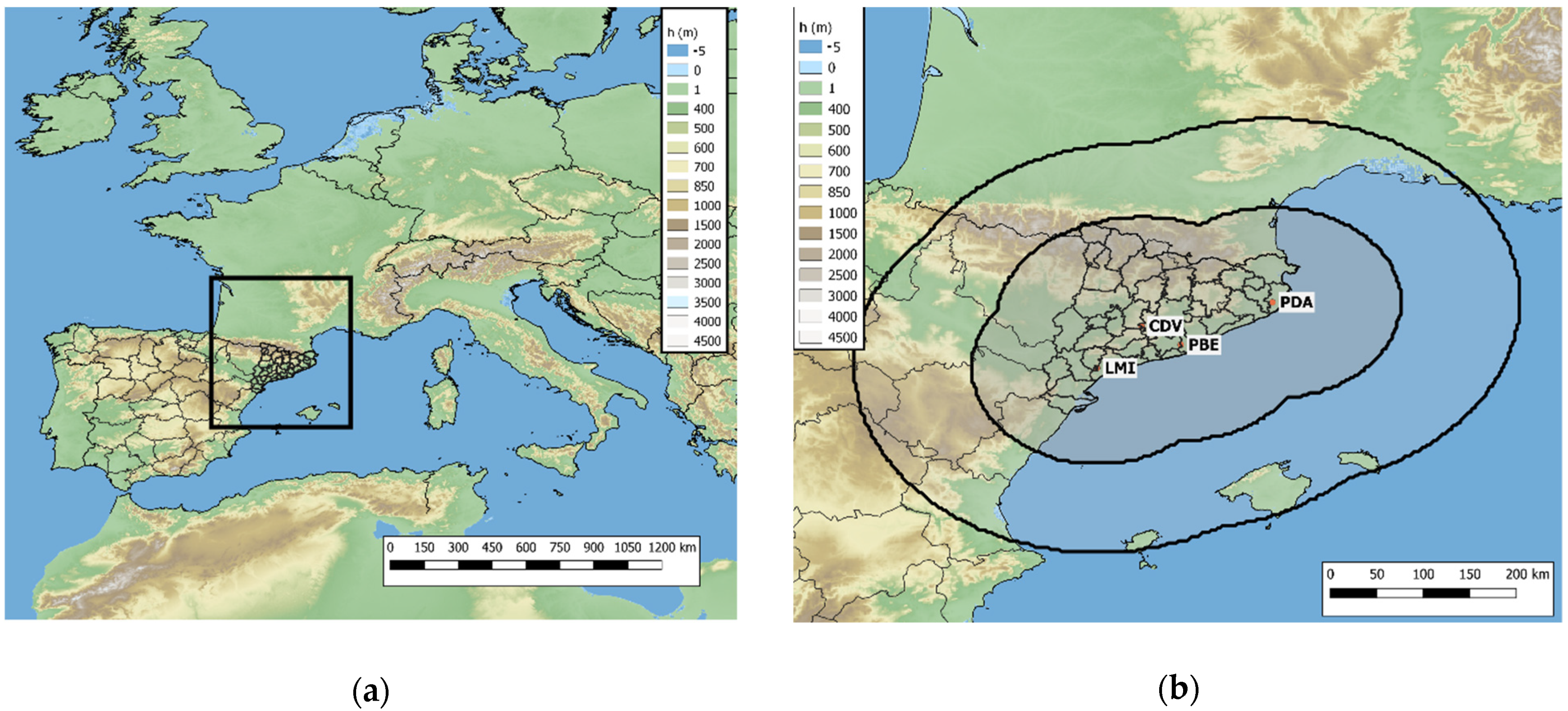
Catalonia is located in the northeasterly part of the Iberian Peninsula (Figure 1a). Because of its topography and location (proximity to the Mediterranean Sea), the region is regularly affected by convective activity that causes severe weather and intense rainfall [18]. This geographical configuration also plays an important role in the fact that numerical weather prediction models have great difficulties in reproducing convective episodes at the scale of thunderstorms [19]. Because of this, using weather radar (XRAD) and rain gauges (XEMA) from automatic weather stations (AWS), the networks provide the results that are strictly necessary for surveillance tasks in the region. This point is further accentuated by the short-time response of most of the drainage basins in the region [20,21].

Figure 1.
(a) Area of interest; (b) XRAD network radar coverage (short and long range). The red dots and labels correspond to the four radars: CDV (Creu del Vent), LMI (La Miranda), PBE (Puig Bernat), and PDA (Puig d’Arques).
Because both of the Meteorological Service of Catalonia (SMC) networks have been widely presented [8,14,20,21], only their main features are briefly introduced here. In the case of the XRAD, it is made up of four single-polarization C-Band Doppler radars (CDV, PBE, PDA, and LMI in Figure 1b) that cover Catalonia and the local areas in two scattering modes (Figure 1b): long (one single low-elevation process generating reflectivity fields from a range of 250 km) and short (15 low- and mid-atmosphere elevations generating volumetric reflectivity fields with a range of 130 km, except CDV radar with a range of 150 km) ranges. The whole process for each radar has a cycle of 6 min, including the antenna returning to its initial position. The entire process, from the volumetric reflectivity raw acquisition to the visualization of the products and the GeoTIFF conversion, is managed using IRIS software [22].
The XEMA network has 181 automatic rain gauges that transmit rainfall information every minute. Considering that Catalonia covers an area of 32,000 km2, the spatial density is one rain gauge per 177 km2. However, the distribution of the AWS is not uniform, meaning that some areas (the more remote and hilly areas) have a lower density of rain gauges. Furthermore, the complexity of the terrain and the influence of the sea means that interpolations using exclusively AWS data are not simple and have many limitations [23].
2.3. Simple Corrections
Except for some specific differences (regarding specific geographic issues: height of the system or proximity to the sea, which is a defining factor in the anomalous propagation of the beam [24]), all the radars in the XRAD network have similar performances including hardware, software, mechanics, electronics, and the programmed elevations. Corrections in this case are based on a series of filters that consider different relationships between quality control parameters depending on the radar variables (more information about the filter process can be found in [14,19]). The final reflectivity field products (COR1 in Figure 2) only remove topographic echoes, but many other non-meteorological echoes remain uncorrected (electromagnetic interferences, bright band effect, beam blockage, wind farms, etc.). The removal process consists of selecting those pixels with a radial velocity equal to zero and converting the reflectivity to null data. The QPE1 results of the application of the classical Marshall–Palmer Z/R relationship is Z = 200R1.6, in which Z (mm6 m−3) is the reflectivity factor and R (mm h−1) is the rainfall rate. Because radar fields measure dBZ (radar reflectivity factor, a logarithmic dimensionless technical unit), the final conversion to QPE is:
where R is the rainfall rate in mm per hour. It is important to note that this relationship has many limitations, mainly in convective rain regimes. However, from the operational experience of the technical staff of the SMC along the years, it has been concluded that applying different constants produces more errors in the final QPE field. One of the main reasons for this is the high variability of the precipitation fields in the region due to the contribution of different factors such as mountains and valleys, the sea, and air masses [1,3]. This variability makes applying more than one relationship generate more errors in the resulting field, which is also confusing for the forecast team. In addition, the short distance between radars (Figure 1b) makes the selection of the relationship possibly even more complex. However, the good radar coverage has many benefits, such as a reduction in the signal attenuation produced by the cores of the thunderstorms or a beam blockage caused by the topography (see the example in Section 3.3), mainly in those regions covered by more than one radar. The time resolution of radar imagery at the SMC is 6 min. Assuming that the rain rate is more or less constant during these 6 min periods, the cumulated precipitation (P6min) for that period results from the instant rain rate R as P6min = R/10. Finally, the total daily accumulation results into QPE = ∑ P6min, with a summation for the entire set of images (240 in total).
R = [(10(dBZ/10))/200]5/8
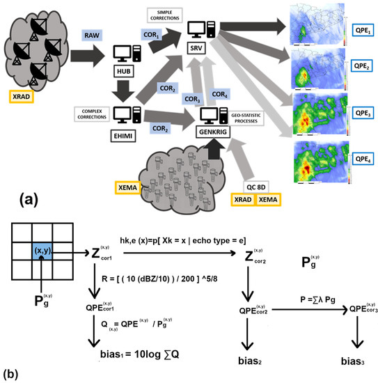
Figure 2.
(a) Diagram of the different QPE processes. (b) Flow chart of the full process scheme.
2.4. EHIMI (Hydrometeorological Integrated Forecasting Tool) Corrections
Since 2004, the SMC, in collaboration with the Catalan Water Agency (ACA) and the Centre of Applied Research on Hydrometeorology (CRAHI), started a project for applying a set of more sophisticated corrections to reflectivity fields [14,25,26]. In 2010, the SMC put the new configuration into operation, the EHIMI (Hydrometeorological Integrated Forecasting Tool), which has been practically unaltered until 2020, except for some minor modifications. The main characteristics of the corrected volumes, COR2, which are also based on the raw files, are fuzzy logic algorithms for removing most non-precipitating echoes. The identification of bright band and the different types of precipitation has made using the vertical profile of reflectivity. This allows for processing of, among other properties: estimating the ground-level reflectivity; removing the main electromagnetic interferences of the most punished azimuths (for which the echoes are removed in the individual radar volumes, avoiding affecting the final composite product); correcting the anomaly associated to partial and total beam blockages at the lowest elevations. In addition, QPE2 generation considers the main flow advection of the reflectivity fields, with the purpose of smoothing the effect of the maxima associated with thunderstorm trajectories. This is the operational product used at the SMC for providing warnings of short periods of heavy rainfall (more than 20 mm in 30 min). The method for estimating the QPE field is the same as that in the previous case but with different reflectivity input maps. Although operationally, the QPE2 is the product used for all hydro-meteorological purposes, the QPE1 remains functioning in real-time for a simple reason: it is the least modified in respect to the original radar measure, allowing for an easier understanding of whether each radar system is functioning well or poorly. The main equation used in the correction procedure, corresponding to the feature histograms (hk,e) for different echo types obtained with the fuzzy logic algorithm, allowing for the identification of meteorological and non-meteorological echoes over land and sea, is:
where n(Xk = x∩ = e) stands for the number of bins, and the echo has been classified as type e; n(e) is the total number of bins classified as echo type e. The possible echo types are precipitation, ground clutter, and sea clutter.
2.5. EHIMI Corrections Combined with Rain Gauge Data
COR2 and QPE2 provide good reflectivity and rain fields from a meteorological point of view. However, another step should be taken to acquire a good compromise for hydrometeorological purposes. This step was a combined effort made in 2010 by ACA and SMC that integrated the AWS rain gauge data of the XEMA network to the previous fields. A preliminary analysis revealed the necessity of applying a correction factor to QPE2, to make it comparable to XEMA values. References [12,13,14] give the main clues to the geostatistical process (in this case, KED or kriging with external drift) for integrating the two sources in a unique field, QPE3, which provides more accurate data for integration in the hydrologic models. However, the main issue of this process is the time delay (~2 h) necessary to include a large number of rain gauge points. This point is important in the region of interest due to the short response for most of the hydrological basins (even less than one hour) and constitutes a key challenge for the future policies of SMC and ACA. The way of estimating the new QPE field considers the rainfall data provided by the rain gauges and includes the effect of the radar with a factor λ for each pixel where ground information exists. Then, the QPE estimated at a certain point results in:
where P(x0, KED) is the rainfall estimated, n is the number of rain gauges used for each point (which is dependent on the spatial distribution of the gauges, and it should be larger or equal to 10), λ(i, KED) is the estimator at the surrounding point xi, and PG is the rainfall measured by the gauge. The estimators or weights are calculated considering the radar variability and the constraint that for the full set of points the sum is one.
2.6. Post-Processed EHIMI Corrections Combined with Rain Gauge Data
The last point in the operative chain is related to quality control of XRAD and XEMA data. Real-time registers can suffer unexpected anomalies caused by different issues. In the case of radar data, the only change made in respect to the previous step consists of re-processing data (this is, to run the software offline generating the products again but with all the data missed in real time) from radars when some volumes have suffered delays in the process of transferring it from the radar to the hub computer (see Figure 2a) at the SMC headquarters or fading [27]. However, XEMA data can suffer many corrections, depending on the characteristics of each gauge (again, problems with communications, under-sampling caused by the topography, evaporation, wind, or funnel losses, among others [28]). The real-time quality control of XEMA data consists in the application of some tests of validation of the different variables, according to a series of thresholds defined based on the experience of the staff who manage the network. Moreover, during the next days after the register, the same staff apply different techniques (such as comparing with radar animations, satellite imagery, lightning data, spotter reports) to validate or change it manually. Once XRAD and XEMA have been processed again, the same technique applied in the previous step runs 8 days later, integrating the new data into a new field, QPE4. Although the product does not have real-time usefulness, it is important from a climatological point of view.
2.7. Bias Estimation
Reference [14] summarizes the process of evaluation for all QPEs generated at the SMC (see Figure 2b). Only a few comments need to be added: the new processing chain generates a GeoTIFF format for all products, making the comparison process between rain gauges and QPE fields easy; all the processes are run on a server computer (SRV in Figure 2a), avoiding differences in formats or changes in projections or resolution; lastly, the SRV computer publishes these products to all users (from the forecast team at the SMC to ACA staff, and many more). The bias compares QPE with ground values and provides information regarding the quality of the products, areas with systematic under-estimation or over-estimation, problems in one radar, and many other points that are fundamental in maintaining the XRAD network. The QPE products generated at the SMC go from 30 min to 24 h accumulation. In this research, only the daily rainfall bias fields are presented.
The daily bias is estimated as follows: First, the QPE radar (Pr) is estimated for each rain gauge location, where the measured rainfall is Pg. The ability of the GeoTIFF format helps to make a more accurate identification of the associated pixel. For each pair of data, the coefficient of the QPE radar estimation for a certain i gauge results in:
Qi = Pri/Pgi
Then, the daily bias results as the evaluation of this factor for the full set of rain gauges with valid information (this is, points closer than 100 km to the radar location and without a quality control flag):
Another advantage of using the GeoTIFF format is the easier definition of the area of validity for the rain gauges around the radar location. The daily bias and the monthly averaged values of the uncorrected QPE field’s (QPE1) result is of great interest for understanding the state of the different radars (under- or over-estimations). If the technician has a good knowledge of the rainfall regimes during the selected period and the calibrating factors of the radar, it is possible to have an accurate idea of the functioning of the systems and to easily and quickly detect possible errors in the radar data acquisition. Once the remote sensing staff have evaluated the different possibilities, maintaining the unit re-calibrates the radar, which is performed systematically at a monthly frequency (but only if it is required). It is also important to say that bias is compared systematically with the root mean square factor (RMSf) to estimate the deviation of the measures, which also is a good indicator of the type of dominant precipitation during the selected period. In any case, the experience over the years on the data analysis has minimized the use of the RMSf, which has a similar behavior according to the period of the year.
3. Results
3.1. Radar Bias Evolution for the Period 2011–2020
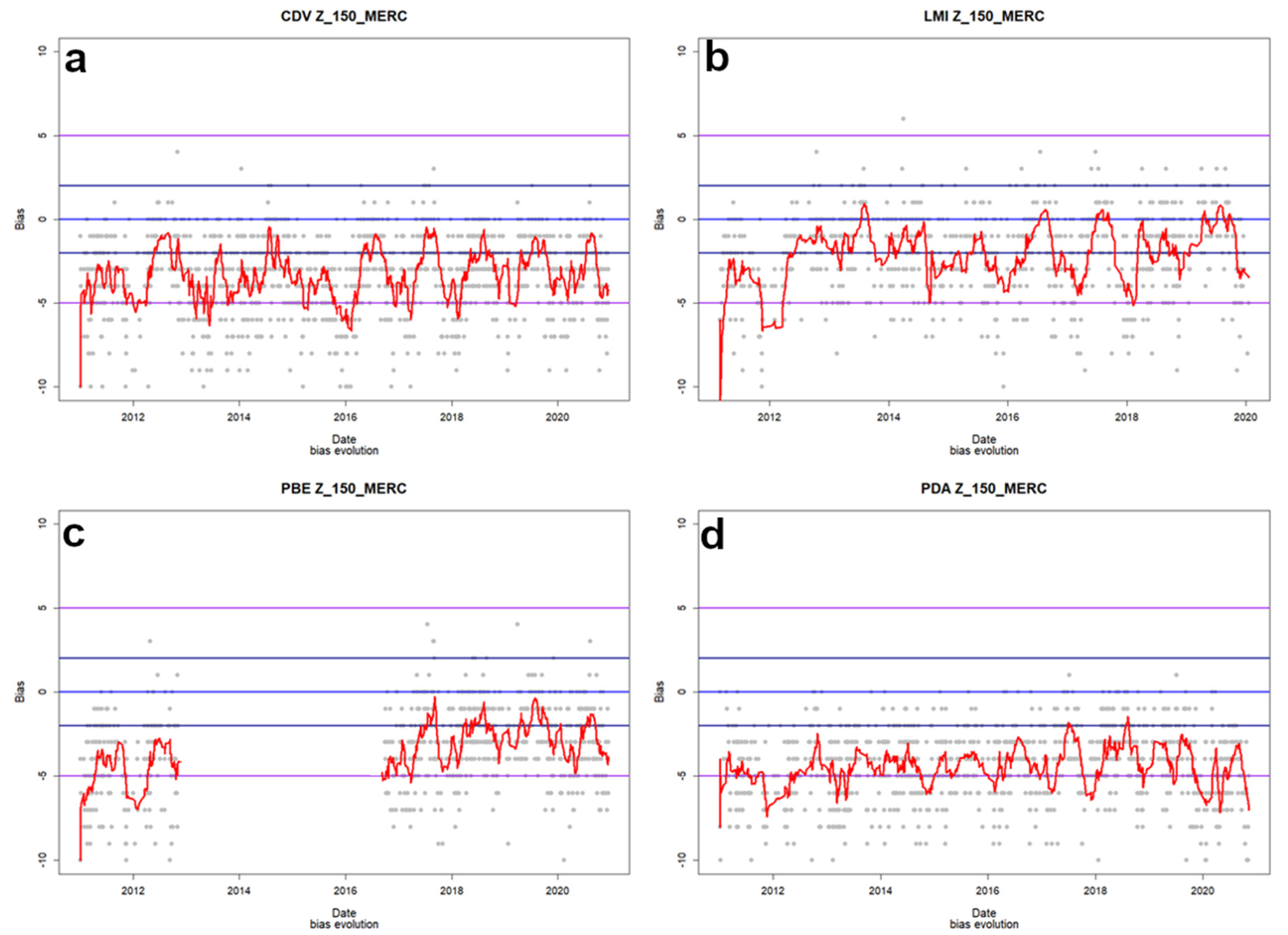
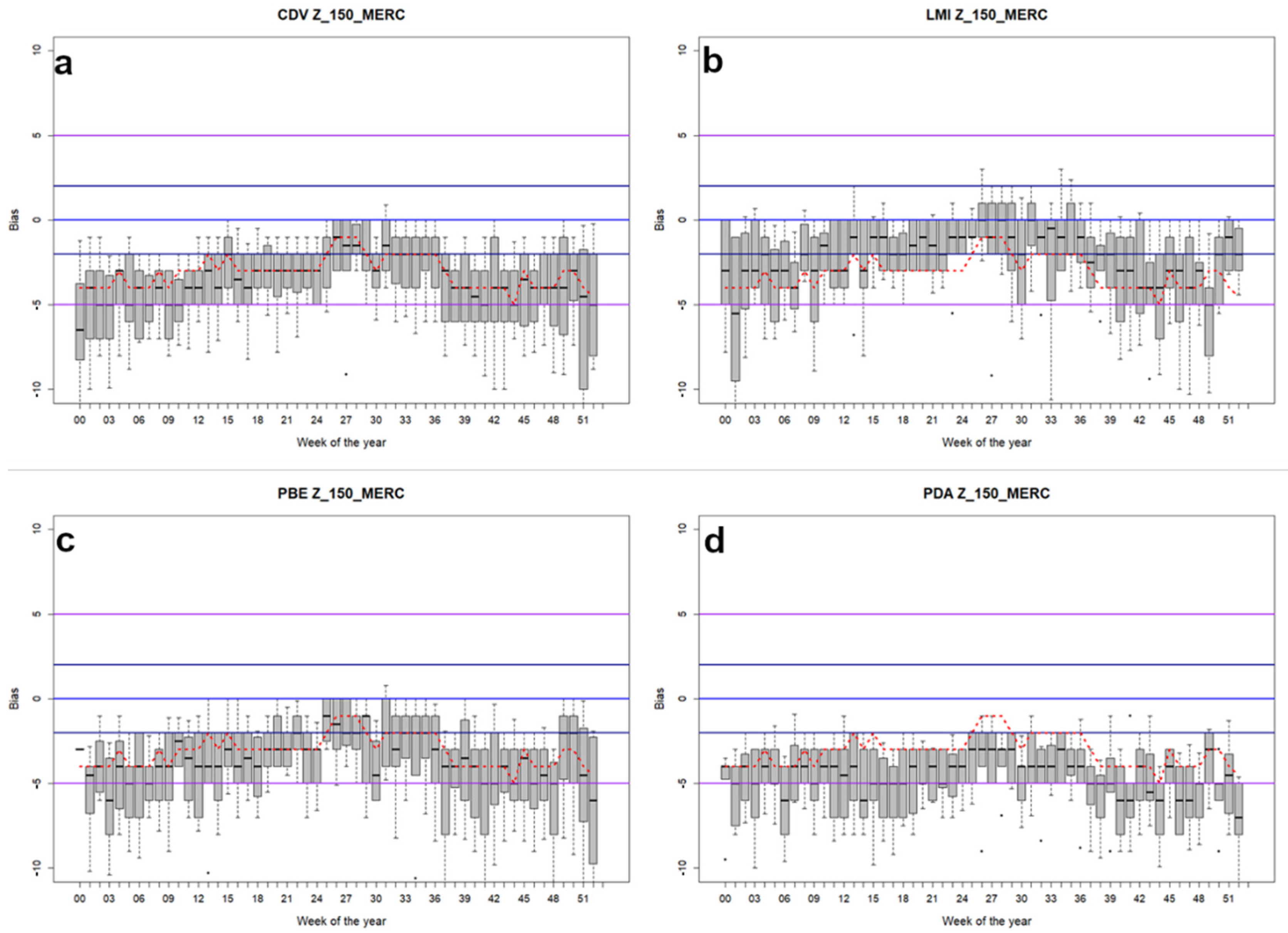
The bias skill score provides useful information regarding the functioning of each XRAD radar. Figure 3 shows the daily evolution of this parameter for the four radars for the 10 year period from 2011–2020 in the case of the QPE1 field (this means with simple corrections). The choice of this product avoids false anomalies caused by the application of corrections that can be minimized when a radar functions poorly (e.g., the data provided does not satisfy the bias quality control in any sense, where the mechanics and electronics have bad pointing accuracy or it is not well-calibrated), at least for a period. The red lines show the 15 day moving average, which smooths anomalous values and superfluous outliers. Keeping in mind that the “perfect bias” corresponds to the zero value (i.e., blue horizontal line) and that acceptable values are between −2 and 2 (i.e., dark blue lines), we can see the continuous under-estimation (i.e., negative values) of all radars. In any case, this trend was not the same across all the radars and, for instance, the LMI showed values closer to zero than the other radars. On the other hand, the PDA presented a clear under-estimation around a value of −5. The lack of data for PBE during the 2013–2016 period was caused by changes in technology, showing a clear improvement in the bias parameter in the second period (from values of approximately −5 to near −2). This first analysis helps us understand the main contribution of each radar to the composite QPEs and, on the other hand, identify possible anomalies in each of the elements of the XRAD network.
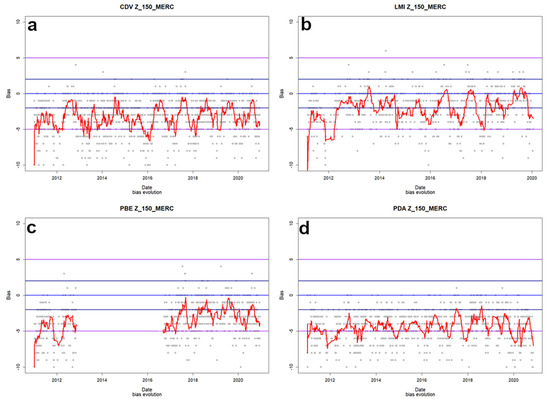
Figure 3.
Bias estimation for a simple QPE of the 4 radars ((a) CDV, (b) LMI, (c) PBE, and (d) PDA) for the 2011–2020 period.
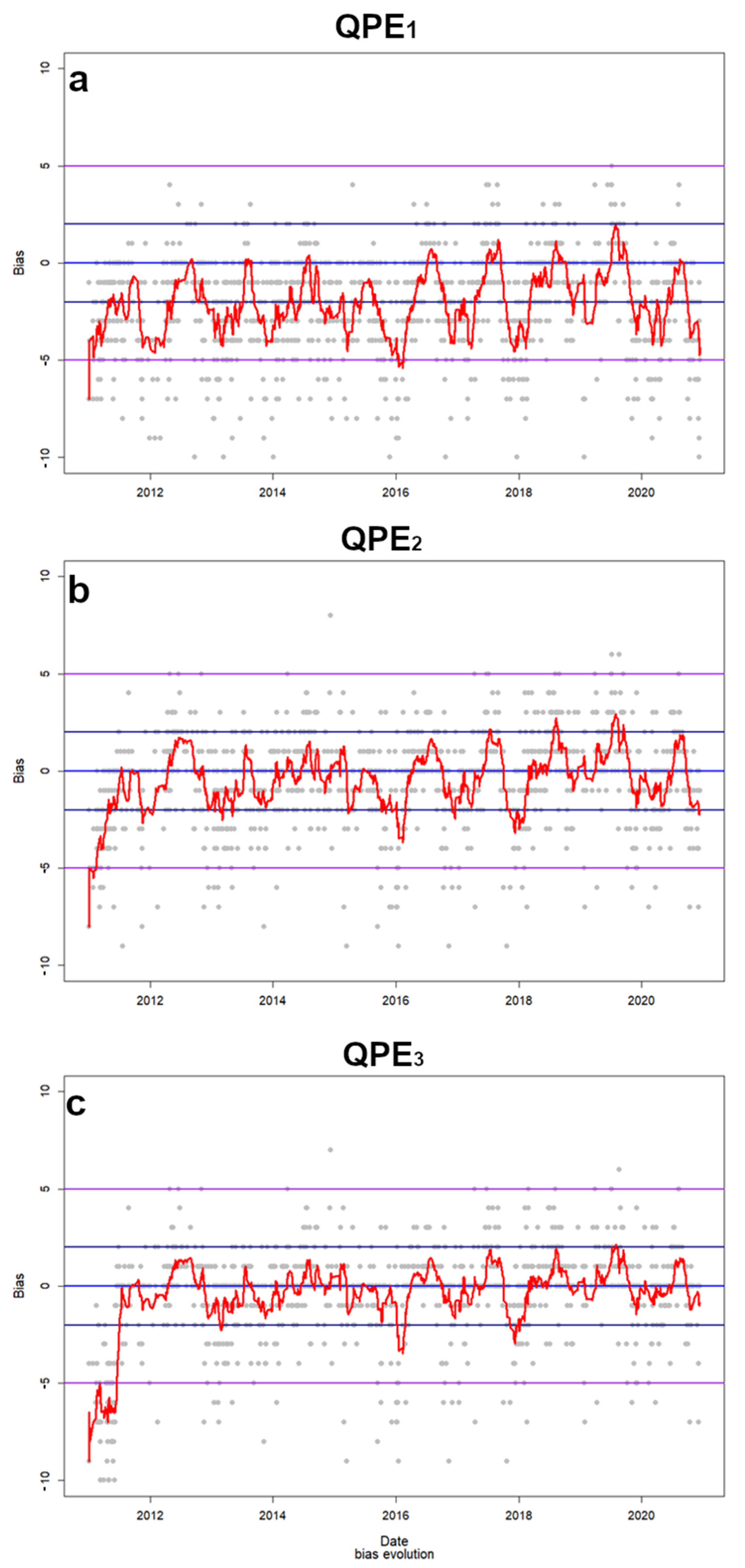
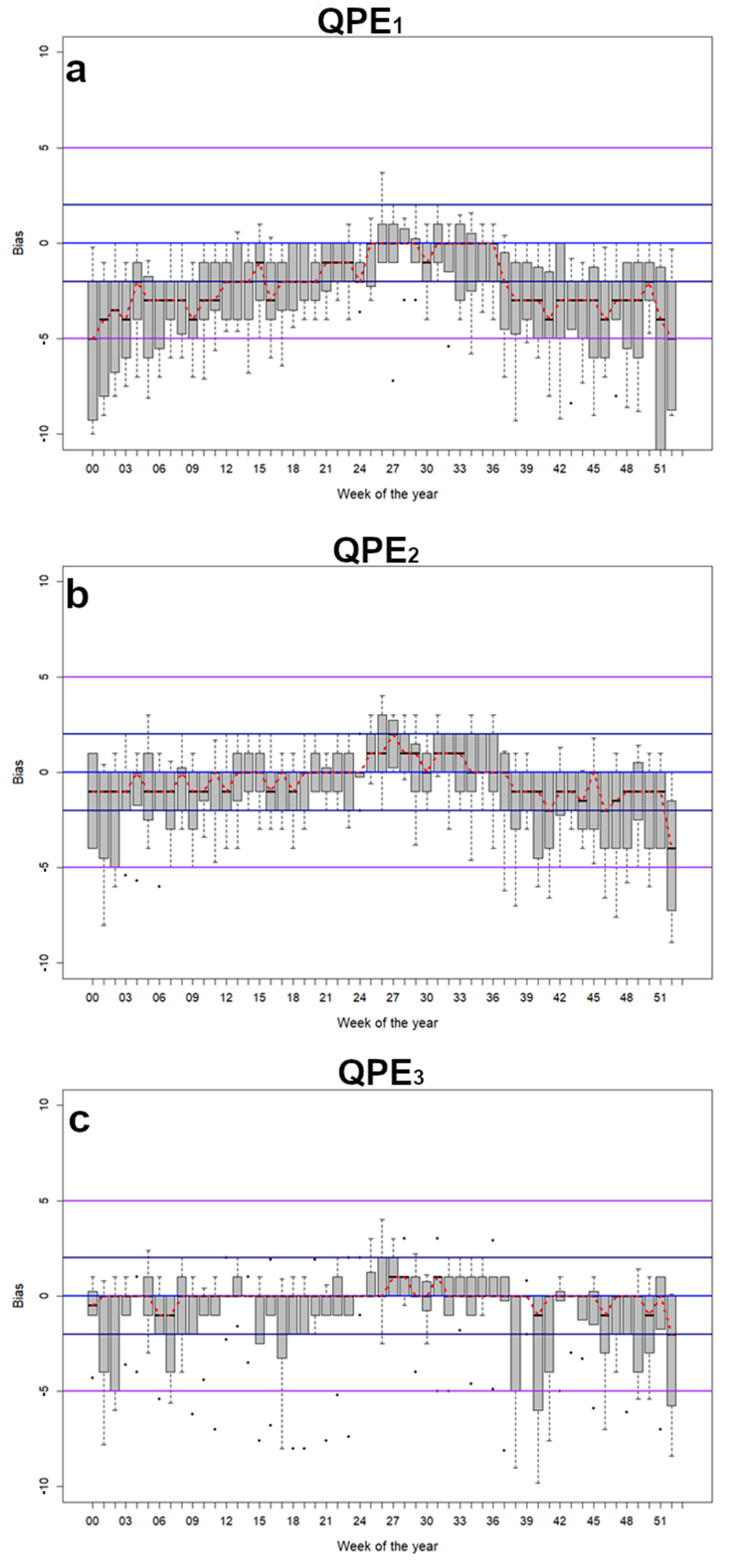
The composite products at the SMC were created by considering the maximum value at each point of the new field obtained from the combination of all the available radars. This penalizes radars underestimating QPE, favoring those that provide more acceptable values. However, this method has limitations, such as a larger influence from the bright band effect, especially in winter events when the melting level is close to some radar heights. Although the correction procedure has a module for reducing this phenomenon, the results are not always satisfactory, and some imagery can present a reflectivity overestimation during winter events. In any case, the number of composites affected by this situation was limited and did not exceed 0.5% of the total annual. Figure 4 shows the bias values for the same period as Figure 3 for the three operational composite QPEs (i.e., QPE1, QPE2, and QPE3). All the composite products showed better bias values than the individual products because of the minimization of the underestimations caused by composites (e.g., a beam blockage that had a negative effect on a concrete area of an individual product was reduced when other radars contributed to that area). However, it shows how the different steps in the correction scheme allowed new fields to be produced with bias values close to zero in most cases. An interesting point was that QPE2 had larger positive bias values than QPE3 in some seasons. This does not mean that the first product had better values, rather that it was more affected by heavy rainfall or hail. Then, the integration of the rain gauges reduced this anomaly. According to the parameters indicated above with respect to better bias behavior, QPE3 generally showed better fitted values, always between −2 and 2 thresholds (except an initial period with some tests that generated unrealistic values).
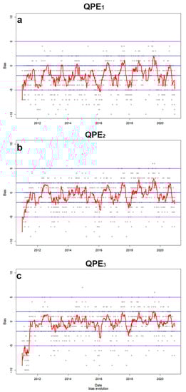
Figure 4.
Same as Figure 3 but for the composite QPE (with simple corrections—panel (a), with EHIMI corrections—panel (b), and with EHIMI plus rain gauge corrections—panel (c)).
Table 2 summarizes the behavior of the seven daily QPE fields for the 2011–2020 period, according to their percentiles (0, 25, 50, 75, and 100). With respect to individual radars, the values indicated the best bias results for LMI and the worst results for PDA, while PBE and CDV showed an intermediate level of quality. This implies that PDA radars contribute less than the average and, on the other hand, LMI appears to provide more to the composite, around the region of influence. Regarding composite products, large differences between QPE1 and QPE2 and QPE3 can be appreciated. These differences are caused by the notable hydrological improvements in the corrections; it is important to be reminded that these corrections are focused on the generation of accurate rain fields, to produce good alerts and assimilations in hydrological models. From this table, it seems that QPE3 did not provide any improvements to the QPE2 field. However, as shown in Figure 4, the values for concrete episodes or periods showed significant differences. These differences will be discussed in the following sections, in the analysis of a concrete event. In any case, the large differences between the QPE estimated by individual radars and the composites with corrections are well reflected in the table.
3.2. The Yearly Cycle of the Bias
Figure 5 and Figure 6 show a boxplot with the weeks of the year (that is, a boxplot of all the values for each week of the year, considering 0 as the first one—from 1 to 7 January, 1 for the second week—8 to 14 January, etc.). In every case, similar behavior can be detected, with minimum values for the period from week 37 to week 12 (cold season) and a maximum for weeks 13 to 36 (warm season). It is worth noting that these were not fixed periods, and it seems the variations were highly dependent on the global temperature of the region and local areas. This means that for years that were colder than average, the cold season will be a bit larger, while, on the other hand, it will be shorter for warmer years. This behavior has a clear relationship with the type of precipitation [29,30]. During cold seasons, scarce to moderate convective regimes dominated, with low to moderate reflectivity values and a clear need for a notable increase in the QPE estimation (bias ranges from −5 in the worst-case scenario, PDA, to −2 in the best QPE1, considering that we excluded the corrected QPEs from this part of the analysis). On the other hand, during the warm season, deep convective regimes with heavy precipitation and hail, should produce large reflectivity values. This implies, in most cases, that values were close to −3 (again, PDA) and 0 (QPE1), indicating that under-estimation was notably reduced during this season.
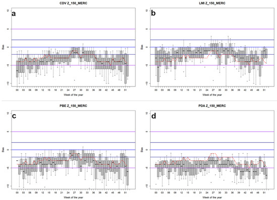
Figure 5.
Boxplot showing weeks of the year and bias for the same radars as in Figure 3 (CDV—(a), LMI—(b), PBE—(c), PDA—(d)). The red, dotted line corresponds to the moving window average for 15 days.
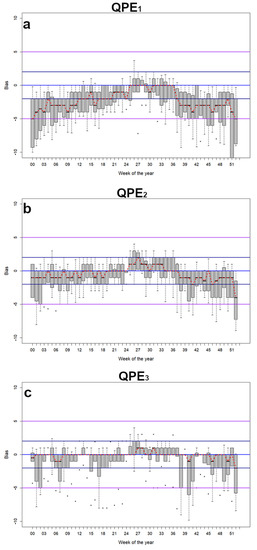
Figure 6.
Boxplot showing weeks of the year and bias for the same composite products as in Figure 4 (with simple corrections—panel (a), with EHIMI corrections—panel (b), and with EHIMI plus rain gauge corrections—panel (c)).
A different case is presented for corrected QPE (QPE2 and QPE3) that shows bias values around zero for the entire year because of corrections. It is important to note that in the case of QPE3 (corrections combined with rain gauges), the effect of the ground data is important, but the product does not provide the exact value of the gauge. This is because the radar field forces the interpolation to adapt to the same pattern of the QPE2. In the case that the value provided by the gauge does not fit with the shape, the interpolation minimizes the effect of the ground data. In any case, a different type of behavior can be appreciated when the XEMA data are included (QPE3), with a smaller range of values between the maximum (1 in front of 2 for QPE2) and the minimum (−1, −2 for QPE2). Moreover, the extreme periods were concentrated in shorter windows. This means that EHIMI corrections, even when notably improving the QPE fields, need contribution from rain gauges for hydrological purposes. This point is better explained with a practical example such as the one given in the following section.
3.3. The Episode of 22 October 2019
On the afternoon and night of 22 October 2019, a very heavy rainfall event produced a dramatic increase in the flow of many small rivers in southern Catalonia. The result of this event was large-scale damage (estimated at more than €700,000) in some villages and, more importantly, four deaths in the region. However, further points in Catalonia were affected by heavy rain (especially in the northeast and central coastal regions), and there was even a tornado (also on the central coast). The QPE fields generated show the large variations depending on the corrections and the source considered (Figure 7, Figure 8, Figure 9 and Figure 10). The GeoTIFF files allow larger differences to be detected, as well as some less evident changes in QPE. All the maps were generated using QGIS [31], a free and open-source cross-platform desktop software geographical information system (GIS).
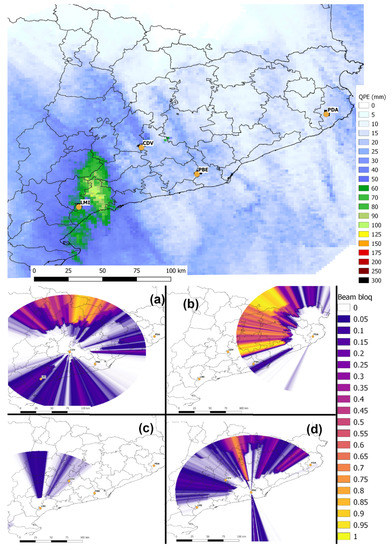
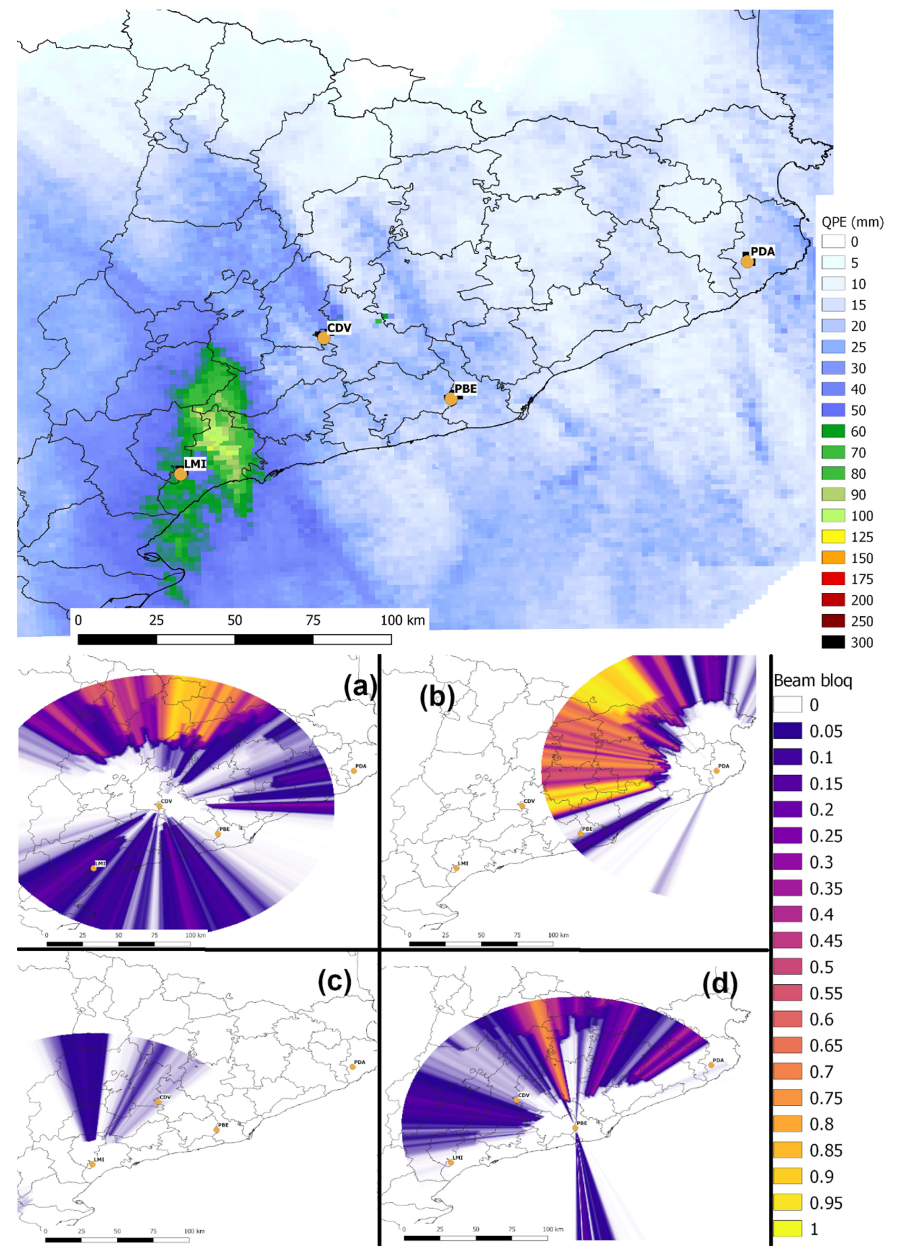
Figure 7.
Top: QPE with simple corrections for the 22 October 2019 event. The orange dots indicate the radar positions. Bottom: Beam blockage matrices for all the four radars at the lower elevations (CDV (a), PDA (b), LMI (c), and PBE (d)).
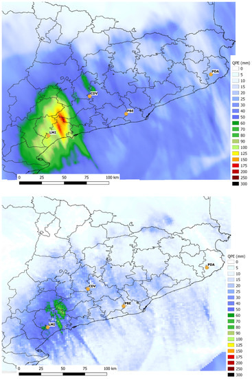
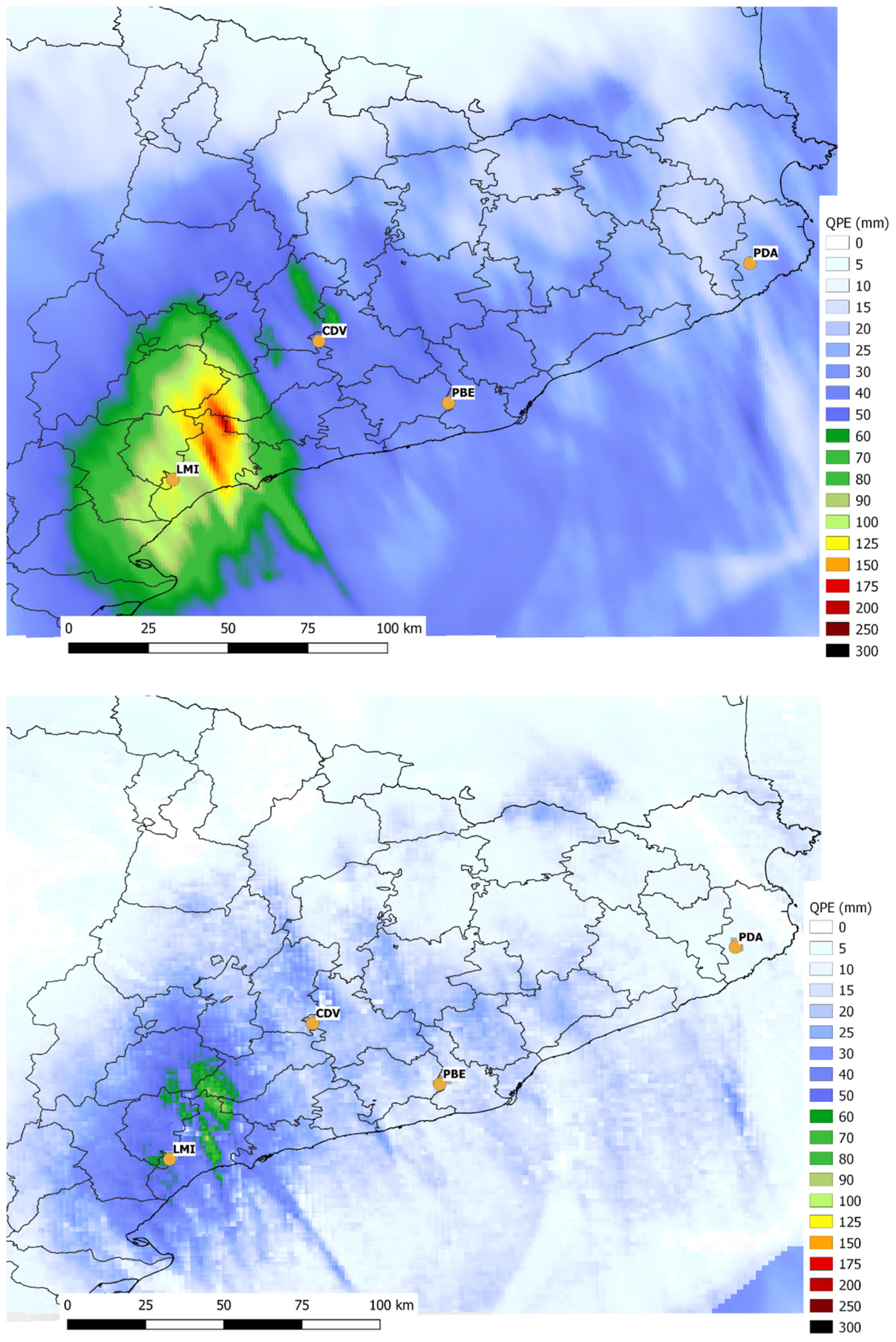
Figure 8.
Top: QPE with complex (EHIMI) corrections for the 22 October 2019 event. Bottom: Difference in the QPE2 field with respect to the uncorrected one, QPE1 (Figure 7).
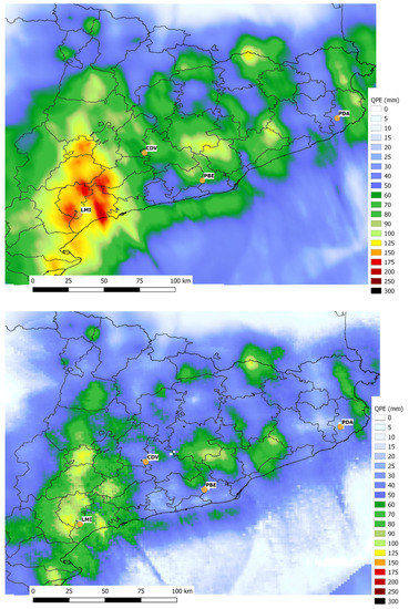
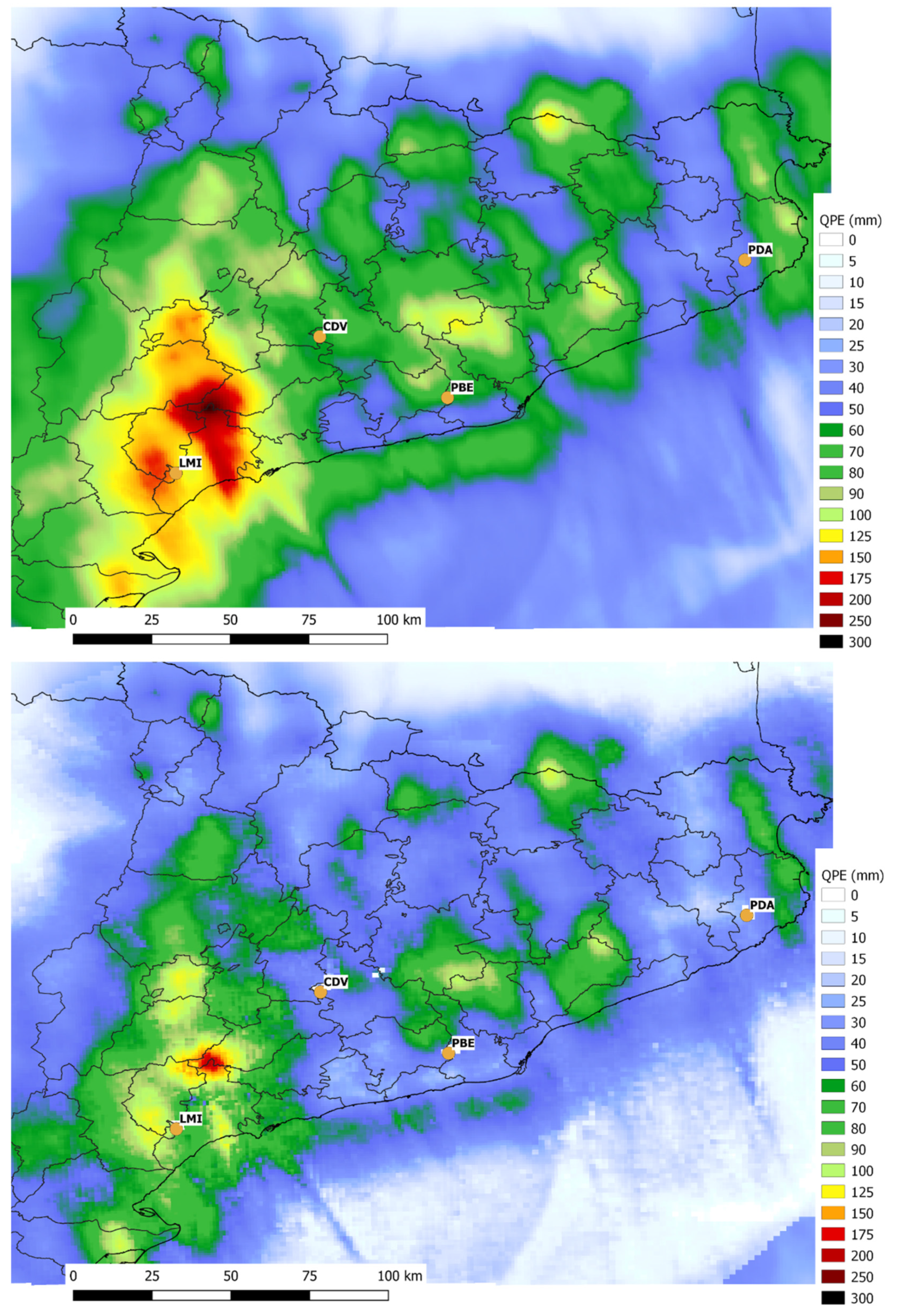
Figure 9.
Top: QPE with EHIMI corrections combined with rain gauge data for the 22 October 2019 event. Bottom: Difference in the QPE3 field with respect to the uncorrected one, QPE1 (Figure 7).
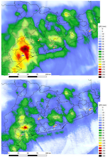
Figure 10.
Top: QPE with EHIMI corrections combined with rain gauge data after the QC process for the 22 October 2019 event. Bottom: Difference in the QPE3 re-processed field (QPE4) with respect to the uncorrected one, QPE1 (Figure 7).
If the only available QPE field was the one with simple corrections (Figure 7, top), one would suppose that the event was important (exceeding 100 mm in 24 h is significant), but it was focused on the area of interest (the southern region), where estimations reached 70 mm in an area of 1800 km2. In the rest of Catalonia, rainfall accumulated values ranged between 5 and 60 mm. Moreover, this figure reveals some limitations, apart from the real estimation of the QPE1: there are important discontinuities in the field caused by the different contributions from each individual radar (the under-estimation of PDA must be remembered, in the northeastern part), the black pixels associated with the position of the different radars, the green pixels in the central part of Catalonia associated with some wind farms, and the clear under-estimation of precipitation in the northern region, caused by the beam blockage (see Figure 7, bottom) of the interaction with mountains exceeding 2500 m. The total maximum value was 111 mm but in a very reduced pixel region (not a robust estimation). According to Figure 7, bottom, (the beam blockage affectation at the lowest beam), the topography did not play a relevant role in the rainfall field, at least in the area with the highest amounts of precipitation. However, it was a negative factor in the northern region, where only the last QPE field was able to estimate the real values of precipitation (see the last part of this section for more details).
Most of the previous limitations in rain fields are drastically reduced when EHIMI corrections were considered (Figure 8, top): the estimation was more continuous in space or local under-estimations were notably reduced. Besides, the values were larger, with an area of 780 km2 exceeding 125 mm, and an area of more than 5300 km2 showing values over 70 mm (three times the QPE1 estimated area for this threshold). Finally, with the exception of the northern part of the region, all of Catalonia recorded values over 40 mm in 24 h. The differences in this field—QPE2—respecting the uncorrected one—QPE1—are shown in Figure 8, bottom, where it is possible to observe how the differences were larger in the area with the highest cumulated values. These records better reflect the description of the event, but considering the nature of other historical cases [17] or the season of the year (between the warm and cold season, which implies an under-estimation of QPE2), QPE3 should be looked at more closely. In this case, the maximum value reached 177 mm, clearly greater in QPE1, and, more importantly, surrounded by other similar values.
Figure 9, top, shows the integration of XEMA and XRAD data, providing the QPE3 field. Again, changes with regard to the previous map are notable. For instance, the total area exceeding 70 mm was close to 20,000 km2 (nearly four times the QPE2 estimation), and many regions exceed 125 mm, mainly in mountainous areas close to the coast. This point is very important from a hydrologic point of view, because the affected basins have a very short time response period of less than one hour (or even less). Otherwise, the last point of note is that the maximum value was 198 mm (20 mm more than for QPE2). Figure 9, bottom, indicates that the gauges’ influence was very important, mainly on those areas with problems caused by the topographic blockage, a part of those regions with the highest cumulated values.
Finally, Figure 10, top, shows QPE4, the final estimation for the episode, obtained 8 days later. Again, there were some changes with respect to the previous map (QPE3). These changes were not as important as in the preliminary steps, but, in any case, they were interesting enough to be noted. Even the general shape of the rainfall field suffered scarce or no changes; in the most-hit area, there were values close to 300 mm (maximum of 282 mm, that is, more than 90 mm more than in the previous case). This large difference was due to the quality control of the XEMA series for some AWS in the affected area. The analysis revealed that it was an under-estimation of the precipitation caused by poor functioning of the sensors as a result of the large amounts of rainfall that accumulated in a few minutes. The comparison with several manual gauges in the region allowed for a reliable evolution of the event in those points, leading to the final map. It is also worthy to note that in the northern and mountainous part of Catalonia, the differences were also evident. In this case, the beam blockage reduced the algorithms capabilities and only the final contribution of the gauges at highest elevations (see Figure 9 and Figure 10, top) helped to produce an accurate rain field.
Using the geostatistical packages of R software [32], such as Raster [33] or MapTools [34], we reprojected and resampled all the fields to the same resolution and projection without losing any spatial information. This process allowed for a simple comparison of the total cumulated precipitation estimated for the entirety of Catalonia (32,000 km2). Table 3 summarizes the differences between the QPE fields through several parameters. In general, all the statistical parameters (sum of the total amount of rainfall pixels—SUM, the mean, and the 90th percentile) indicate the same behavior, doubling values of QPE2 compared to QPE1, and for QPE3 over QPE2. These results show the importance of corrections in the rainfall field. This doubling trend was not observed in the case of QPE4 and QPE3, where the differences were subtle (one mm in the case of the mean or 0.3 mm for Q0.90). However, if we analyze areas exceeding a certain threshold (in this case, 100 and 200 mm), crude variations between all the fields are shown. QPE1 shows a small area exceeding the first threshold and none for the second one. The last value (0 pixels exceeding 200 mm) is also shown in the case of QPE2 and QPE3, while only QPE4 showed an area of 190 km2 with values over that value. In the case of the 100 mm threshold, the change between QPE1 and QPE2 was 2677.3% and 302.1% for QPE2 and QPE3. In the latter case, the variation was reduced to 1.1%.
Table 3.
Different parameters (from left to right: total sum of rainfall for all pixels 1 × 1 km2 with precipitation over Catalonia; mean rainfall value for the same set of pixels; 90th percentile; number of pixels with QPE over 100 mm; number of pixels with QPE over 200 mm) obtained for geostatistical analysis of the GeoTIFF files associated with each QPE field for the 22 October 2019 event.
4. Discussion
The purpose of this research was to show the capabilities of GeoTIFF format files to analyze the quality control of weather radar data and to monitor and understand heavy rainfall events from a meteorological point of view. The change in the data format of the QPE files used in the bias estimation for each of the radar products allowed for the simplification of the process and, more importantly, avoided issues in terms of changes in the location of the calibration points. The georeferenced files made it easier to compare rainfall field and ground observations. This point was crucial when putting the process into operation in near real-time (the script generates the bias values 2 h after the last product arrives to the SRV computer, considering that QPE4 was not analyzed with this methodology).
Generating the QPE products in real time was very helpful in terms of maintaining the XRAD network, because it allowed us to detect anomalies in radar behavior. However, the yearly variation of the factor must be considered, which is highly dependent on the type of precipitation and the season in question (warm, cold, and transition period). This behavior was observed in other meteorological issues in the region such as the occurrence and intensity of mesoscale convective systems (MCS, [35]). Research has shown some examples of anomalies in the different radars of the XRAD network. Moreover, it has presented normal functioning interval values for all the radars and, also, of the different composite products (with simple corrections, with EHIMI corrections, and with EHIMI plus XEMA corrections).
The differences among all the QPE fields were evident, and they showed the importance of the contributions of the different algorithms (i.e., EHIMI corrections, rain gauges data interpolation, and quality control integration) to rainfall estimation. The understanding of the corrections’ influence is crucial, mainly for hydrological purposes, because the changes caused by each one of the different algorithms affect the input field into the models. However, future research could integrate QPE data in a hydrological model, to show the differences in outputs. In any case, from the feedback provided by the ACA staff in the flood emergency plan for Catalonia (INUNCAT, [17]), we know that the time response of many of the Catalan basins is to the order of one hour or even less (in particular for coastal areas). We must therefore evaluate the previous results from a different perspective, that is, from a surveillance point of view. Disregarding the QPE4 for obvious reasons, we focused on the other three products (i.e., QPE1, QPE2, and QPE3). The first was generated in just a few seconds, when the technician received the GeoTIFF file or the imagery five minutes later than in real time because of processing the entire raw volumes used to generate the rainfall field. A few seconds later (nearly 30 s later), EHIMI generated QPE2 and sent it to the SRV computer. It was evident that the improvement shown in the preliminary section makes QPE2 more useful than QPE1. However, at the time of evaluating QPE3, the good results shown earlier were masked by the time it took for the product to be generated. This is hardly sensitive to the type of precipitation, and it needs a large set of rain gauge data (more than 80%). The current process at the SMC indicates that the generation period is between 30 min (optimal time) and 3 h (worst scenario). Considering the previous hydrological time constraint, it is clear that QPE3 has limited usefulness for real-time processes.
In any case, both QPE3 and QPE4 have many uses, such as bias estimation or the quantification of heavy rainfall events, as previously presented. In addition, the use of GeoTIFF files is very helpful when investigating the rain characteristics of the event, through tools, such as GIS, or software such as R. Different techniques help to understand the nature of the event and improve disaster mitigation techniques.
5. Conclusions
The use of the GeoTIFF format allowed for real-time procedures to be generated for analysis of the quality of QPE data from each radar on the XRAD network. The fact that this format generates files of smaller size without losing quality of the data helps to archive and manage large amounts of data easily. Moreover, different composite products are analyzed daily, compared with rain gauge data. This process allows poorly functioning radars to be detected or regions to be identified with systematic under-estimations of QPE because of different factors (mainly geographic and environmental conditions). It is also interesting to conclude the importance of the geo-statistical processes in the correction of the QPE, including the high role of the rain gauge data, which combined with the corrected field estimated by the radar, allows generating a final product with a high potential for hydro-meteorological purposes.
We defined the quality values for all four radars and for the three main composite products. These thresholds will be put into operation as a system that warns of possible anomalies in the QPE generated. However, as presented above, the seasonal factor must be considered before deciding to make an intervention in a radar or change the parameters of an algorithm.
Finally, GeoTIFF files have been especially useful when analyzing individual episodes, allowing us to detect the performance of a product by means of different geostatistical procedures. This analysis is very helpful when detecting weak points in current warning systems in civil protection emergency plans, making it easier to improve.
Author Contributions
Conceptualization, T.R., L.E. and M.C.L.; methodology, T.R.; software, T.R. and L.E.; validation, T.R.; formal analysis, T.R., M.C.L. and L.E.; investigation, T.R., M.C.L. and L.E.; resources, M.C.L.; data curation, L.E.; writing—original draft preparation, T.R.; writing—review and editing, T.R., M.C.L. and L.E.; visualization, T.R. and L.E.; supervision, M.C.L.; project administration, T.R. and M.C.L.; funding acquisition, M.C.L. All authors have read and agreed to the published version of the manuscript.
Funding
This work was carried out in the framework of the M-CostAdapt (CTM2017-83655-C2-1&2-R) research project, funded by the Spanish Ministry of Economy and Competitiveness (MINECO/AEI/FEDER, UE).
Institutional Review Board Statement
Not applicable.
Informed Consent Statement
Not applicable.
Acknowledgments
The authors want to thank to the SMC and ACA for the data provided and their comments.
Conflicts of Interest
The authors declare no conflict of interest.
References
- Llasat, M.C.; Rigo, T.; Villegas, J.J. Techniques and instruments to aid in the monitoring of flood events. In Floods; Vinet, F., Ed.; Elsevier: Amsterdam, The Netherlands, 2017. [Google Scholar]
- Hally, A.; Caumont, O.; Garrote, L.; Richard, E.; Weerts, A.; Delogu, F.; Fiori, E.; Rebora, N.; Parodi, A.; Mihalović, A.; et al. Hydrometeorological multi-model ensemble simulations of the 4 November 2011 flash flood event in Genoa, Italy, in the framework of the DRIHM project. Nat. Hazards Earth Syst. Sci. 2015, 15, 537–555. [Google Scholar] [CrossRef] [Green Version]
- Álvarez-Rodríguez, J.; Llasat, M.C.; Estrela, T. Analysis of geographic and orographic influence in Spanish monthly precipitation. Int. J. Clim. 2017, 37, 350–362. [Google Scholar] [CrossRef]
- Diez-Sierra, J.; del Jesus, M. A rainfall analysis and forecasting tool. Environ. Model. Softw. 2017, 97, 243–258. [Google Scholar] [CrossRef]
- Germann, U.; Berenguer, M.; Sempere-Torres, D.; Zappa, M. Real—Ensemble radar precipitation estimation for hydrology in a mountainous region. Q. J. R. Meteorol. Soc. 2009, 135, 445–456. [Google Scholar] [CrossRef] [Green Version]
- Doviak, R.J.; Zrnić, D.S. Doppler Radar and Weather Observations, 2nd ed.; Academic Press: Cambridge, MA, USA, 1993. [Google Scholar]
- Bech, J.; Codina, B.; Lorente, J.; Bebbington, D. The sensitivity of single polarization weather radar beam blockage correction to variability in the vertical refractivity gradient. J. Atmos. Ocean. Technol. 2003, 20, 845–855. [Google Scholar] [CrossRef] [Green Version]
- Altube, P.; Bech, J.; Argemí, O.; Rigo, T. Quality control of antenna alignment and receiver calibration using the sun: Adaptation to midrange weather radar observations at low elevation angles. J. Atmos. Ocean. Technol. 2015, 32, 927–942. [Google Scholar] [CrossRef] [Green Version]
- Nilsson, C.; Dokter, A.M.; Verlinden, L.; Shamoun-Baranes, J.; Schmid, B.; Desmet, P.; Bauer, S.; Chapman, J.; Alves, J.A.; Stepanian, P.M.; et al. Revealing patterns of nocturnal migration using the European weather radar network. Ecography 2018, 42, 876–886. [Google Scholar] [CrossRef] [Green Version]
- Wagner, P.; Fiener, P.; Wilken, F.; Kumar, S.; Schneider, K. Comparison and evaluation of spatial interpolation schemes for daily rainfall in data scarce regions. J. Hydrol. 2012, 464–465, 388–400. [Google Scholar] [CrossRef]
- Dirks, K.; Hay, J.; Stow, C.; Harris, D. High-resolution studies of rainfall on Norfolk Island: Part II: Interpolation of rainfall data. J. Hydrol. 1998, 208, 187–193. [Google Scholar] [CrossRef]
- Velasco-Forero, C.A.; Sempere-Torres, D.; Cassiraga, E.; Gómez-Hernández, J.J. A non-parametric automatic blending methodology to estimate rainfall fields from rain gauge and radar data. Adv. Water Resour. 2009, 32, 986–1002. [Google Scholar] [CrossRef]
- Schiemann, R.; Erdin, R.; Willi, M.; Frei, C.; Berenguer, M.; Sempere-Torres, D. Geostatistical radar-raingauge combination with nonparametric correlograms: Methodological considerations and application in Switzerland. Hydrol. Earth Syst. Sci. 2011, 15, 1515–1536. [Google Scholar] [CrossRef] [Green Version]
- Trapero, L.; Bech, J.; Rigo, T.; Pineda, N.; Forcadell, D. Uncertainty of precipitation estimates in convective events by the Meteorological Service of Catalonia radar network. Atmos. Res. 2009, 93, 408–418. [Google Scholar] [CrossRef]
- Tabary, P.; Boumahmoud, A.-A.; Andrieu, H.; Thompson, R.J.; Illingworth, A.J.; Le Bouar, E.; Testud, J. Evaluation of two “integrated” polarimetric quantitative precipitation estimation (QPE) algorithms at C-band. J. Hydrol. 2011, 405, 248–260. [Google Scholar] [CrossRef]
- Marra, F.; Morin, E. Use of radar QPE for the derivation of intensity–duration–frequency curves in a range of climatic regimes. J. Hydrol. 2015, 531, 427–440. [Google Scholar] [CrossRef]
- Llasat, M.C.; Llasat-Botija, M.; Rodriguez, A.; Lindbergh, S.; Llasat, M.C.; Llasat-Botija, M.; Rodriguez, A.; Lindbergh, S. Flash floods in Catalonia: A recurrent situation. Adv. Geosci. 2010, 26, 105–111. [Google Scholar] [CrossRef] [Green Version]
- Moral, A.; del Carmen Llasat, M.; Rigo, T. Connecting flash flood events with radar-derived convective storm characteristics on the northwestern Mediterranean coast: Knowing the present for better future scenarios adaptation. Atmos. Res. 2020, 238, 104863. [Google Scholar] [CrossRef]
- Moral, A.; Weckwerth, T.M.; Rigo, T.; Bell, M.M.; Llasat, M.C. C-band dual-doppler retrievals in complex terrain: Improving the knowledge of severe storm dynamics in catalonia. Remote Sens. 2020, 12, 2930. [Google Scholar] [CrossRef]
- Amengual, A.; Romero, R.; Gomez, M.; Martin, A.; Alonso, S. A hydrometeorological modeling study of a flash-flood event over catalonia, Spain. J. Hydrometeorol. 2007, 8, 282–303. [Google Scholar] [CrossRef] [Green Version]
- Pascual, D.; Pla, E.; Lopez-Bustins, J.A.; Retana, J.; Terradas, J.; Sanchez, D.P. Impacts of climate change on water resources in the Mediterranean Basin: A case study in Catalonia, Spain. Hydrol. Sci. J. 2015, 60, 2132–2147. [Google Scholar] [CrossRef] [Green Version]
- Skripniková, K.; Řezáčová, D. Comparison of radar-based hail detection using single- and dual-polarization. Remote Sens. 2019, 11, 1436. [Google Scholar] [CrossRef] [Green Version]
- Ninyerola, M.; Pons, X.; Roure, J.M. Monthly precipitation mapping of the Iberian Peninsula using spatial interpolation tools implemented in a geographic information system. Theor. Appl. Clim. 2006, 89, 195–209. [Google Scholar] [CrossRef] [Green Version]
- Bebbington, D.; Rae, S.; Bech, J.; Codina, B.; Picanyol, M. Modelling of weather radar echoes from anomalous propagation using a hybrid parabolic equation method and NWP model data. Nat. Hazards Earth Syst. Sci. 2007, 7, 391–398. [Google Scholar] [CrossRef] [Green Version]
- Berenguer, M.; Sempere-Torres, D.; Corral, C.; Sánchez-Diezma, R. A fuzzy logic technique for identifying nonprecipitating echoes in radar scans. J. Atmos. Ocean. Technol. 2006, 23, 1157–1180. [Google Scholar] [CrossRef] [Green Version]
- Franco, M.; Sánchez-Diezma, R.; Sempere-Torres, D. Improvements in weather radar rain rate estimates using a method for identifying the vertical profile of reflectivity from volume radar scans. Meteorol. Z. 2006, 15, 521–536. [Google Scholar] [CrossRef]
- Panagopoulos, A.D.; Kanellopoulos, J.D. On the rain attenuation dynamics: Spatial-temporal analysis of rainfall rate and fade duration statistics. Int. J. Satell. Commun. Netw. 2003, 21, 595–611. [Google Scholar] [CrossRef]
- Devine, K.A.; Mekis, E. Field accuracy of Canadian rain measurements. Atmos. Ocean 2008, 46, 213–227. [Google Scholar] [CrossRef]
- Rigo, T.; Berenguer, M.; Llasat, M.D.C. An improved analysis of mesoscale convective systems in the western Mediterranean using weather radar. Atmos. Res. 2019, 227, 147–156. [Google Scholar] [CrossRef]
- Llasat, M.C. An objective classification of rainfall events on the basis of their convective features: Application to rainfall intensity in the northeast of Spain. Int. J. Climatol. 2001, 21, 1385–1400. [Google Scholar] [CrossRef]
- QGIS Development Team. Geographic Information System. QGIS Association. 2020. Available online: http://www.qgis.org/ (accessed on 10 April 2021).
- R Core Team. R: A Language and Environment for Statistical Computing. Available online: https://www.R-project.org/ (accessed on 14 April 2021).
- Hijmans, R.J. Raster: Geographic Data Analysis and Modeling. Available online: https://CRAN.R-project.org/package=raster (accessed on 16 April 2021).
- Bivand, R.; Lewin-Koh, N. Maptools: Tools for Handling Spatial Objects. R Package Version 0.9-9. 2019. Available online: https://CRAN.R-project.org/package=maptools (accessed on 16 April 2021).
- Rigo, T.; Llasat, M.-C. Analysis of mesoscale convective systems in Catalonia using meteorological radar for the period 1996–2000. Atmos. Res. 2007, 83, 458–472. [Google Scholar] [CrossRef]


Publisher’s Note: MDPI stays neutral with regard to jurisdictional claims in published maps and institutional affiliations. |
© 2021 by the authors. Licensee MDPI, Basel, Switzerland. This article is an open access article distributed under the terms and conditions of the Creative Commons Attribution (CC BY) license (https://creativecommons.org/licenses/by/4.0/).