Abstract
The rapid rise of ultra-low-cost dual-frequency GNSS chipsets and micro-electronic-mechanical-system (MEMS) inertial sensors makes it possible to develop low-cost navigation systems, which meet the requirements for many applications, including self-driving cars. This study proposes the use of a dual-frequency u-blox F9P GNSS receiver with xsens MTi670 industrial-grade MEMS IMU to develop an ultra-low-cost tightly coupled (TC) triple-constellation GNSS PPP/INS integrated system for precise land vehicular applications. The performance of the proposed system is assessed through comparison with three different TC GNSS PPP/INS integrated systems. The first system uses the Trimble R9s geodetic-grade receiver with the tactical-grade Stim300 IMU, the second system uses the u-blox F9P receiver with the Stim300 IMU, while the third system uses the Trimble R9s receiver with the xsens MTi670 IMU. An improved robust adaptive Kalman filter is adopted and used in this study due to its ability to reduce the effect of measurement outliers and dynamic model errors on the obtained positioning and attitude accuracy. Real-time precise ephemeris and clock products from the Centre National d’Etudes Spatials (CNES) are used to mitigate the effects of orbital and satellite clock errors. Three land vehicular field trials were carried out to assess the performance of the proposed system under both open-sky and challenging environments. It is shown that the tracking capability of the GNSS receiver is the dominant factor that limits the positioning accuracy, while the IMU grade represents the dominant factor for the attitude accuracy. The proposed TC triple-constellation GNSS PPP/INS integrated system achieves sub-meter-level positioning accuracy in both of the north and up directions, while it achieves meter-level positioning accuracy in the east direction. Sub-meter-level positioning accuracy is achieved when the Stim300 IMU is used with the u-blox F9P GNSS receiver. In contrast, decimeter-level positioning accuracy is consistently achieved through TC GNSS PPP/INS integration when a geodetic-grade GNSS receiver is used, regardless of whether a tactical- or an industrial-grade IMU is used. The root mean square (RMS) errors of the proposed system’s attitude are about 0.878°, 0.804°, and 2.905° for the pitch, roll, and azimuth angles, respectively. The RMS errors of the attitude are significantly improved to reach about 0.034°, 0.038°, and 0.280° for the pitch, roll, and azimuth angles, respectively, when a tactical-grade IMU is used, regardless of whether a geodetic- or low-cost GNSS receiver is used.
1. Introduction
GNSS precise point positioning (PPP) is capable of providing precise positioning solutions without any additional GNSS base stations [1]. A costly geodetic grade GNSS device is required for PPP to achieve precise positioning, which limits the use of PPP in a wide range of commercial applications. The release of dual-frequency (DF) GNSS smartphones such as Xiaomi mi 8, which supports dual-frequency (DF) GNSS measurements, allowed users to remove the ionospheric delay, which in turn led to an enhanced PPP solution [2]. It has been shown in [3,4] that DF PPP through smartphones can achieve positioning accuracy at the decimeter to sub-meter-level in static mode. However, their PPP accuracy is degraded to two-meter level in kinematic mode [5]. Low-cost dual-frequency GNSS modules have recently become available, including the u-blox F9P module [6]. This, in turn, increases the potential to provide high positioning accuracy at a fraction of the cost. Unfortunately, however, GNSS-based positioning is vulnerable to partial or full blockage of the GNSS signal in challenging environments such as downtown areas and tunnels [7]. This, in turn, may cause accuracy degradation or unavailability of the GNSS-based positioning solution. Inertial navigation system (INS), on the other hand, is an autonomous system that provides navigation solutions without being affected by the surrounding environment. However, accumulated accelerometer and gyroscope errors over time, particularly when a micro-electro-mechanical system (MEMS) sensor is used, lead to significant drifts in the navigation solution [8]. To overcome the drawbacks of each system and provide continuous and accurate positioning and attitude solutions, the GNSS/INS integration has been developed. Through this integration, GNSS constrains the inertial-based solution drift, while the INS provides continuous positioning and attitude solutions when the GNSS solution is either degraded or not available due to partial or complete GNSS outages.
GNSS PPP/INS integration can generally be performed in a loosely coupled [9], a tightly coupled [10], or an ultra-tightly coupled mode [11]. Tightly coupled integration has the advantage of being able to provide continuous updates to the estimation filter during periods of poor satellite visibility compared to the loosely coupled integration [12]. Ultra-tight integration, on the other hand, requires access to the internal GNSS receiver hardware, which may not be possible for end-users. Tightly coupled (TC) GNSS PPP/MEMS-based INS integration has been addressed by many researchers for land vehicular navigation [10,12,13,14]. In [10], TC GPS PPP/INS integration algorithms were developed using a Trimble R10 geodetic receiver and a NovAtel CPT-IMU. Decimeter-level positioning accuracy was obtained with full satellite availability and a simulated GPS outage of up to 10 s, while a maximum positioning error at the meter-level was obtained when a simulated 60 s GPS outage was applied. TC multi-constellation GNSS PPP/INS integration was assessed through a land vehicular experiment [13]. It was shown that the positioning accuracy of the TC GNSS PPP/INS integration was significantly improved when GPS, GLONASS, Galileo, and BeiDou observations were utilized, in comparison with the TC GPS PPP/INS integration counterpart. Additionally, a minor improvement in the accuracy of the velocity and attitude solutions was achieved through the TC multi-constellation GNSS PPP/INS integration. A TC, ambiguity-fixed GNSS PPP/INS solution was compared to the float-ambiguity counterpart through two real-test scenarios using a NovAtel OEM4 geodetic-grade receiver and LCI tactical-grade IMU [15]. The positioning accuracy was significantly improved through the TC ambiguity-fixed GNSS PPP/INS integration. However, the velocity and attitude solutions of both of the float- and ambiguity-fixed TC GNSS PPP/INS integration were comparable. The extended Kalman filter (EKF) has been commonly used for TC GNSS PPP/INS integration algorithms. Different estimation filters were used by many studies, including the robust Kalman filter RKF [14], unscented Kalman filter (UKF) [16], unscented particle filter (UPF) [17], extended particle filter (EPF) [16], and particle filter (PF) [18]. In [14], a TC GNSS/INS integration algorithm through the RKF was developed using the NovAtel OEM3 geodetic-grade receiver and Stim300 tactical-grade IMU. It was shown that the positioning accuracy was improved significantly through the RKF compared to the conventional EKF.
In the above-mentioned studies, geodetic-grade GNSS receivers were used with tactical-grade IMUs to provide precise positioning and attitude solutions. The cost issue of the integrated system was addressed through the use of a single-frequency (SF) GNSS chipset along with a consumer-grade IMU [19] as well as through the implementation of a reduced inertial sensor system (RISS), as opposed to a full IMU [20]. In [19], a loosely coupled (LC) SF GNSS PPP/INS integrated system was assessed for land vehicular navigation. Their system used the low-cost u-blox EVK-8MT SF GNSS chipset along with the LSM6DSL consumer-grade IMU. In that study, the CNES real-time ionosphere products were used to mitigate the ionospheric delay. The proposed system achieved sub-meter-level horizontal accuracy and meter-level vertical positioning accuracy under an open-sky environment. Additionally, meter-level positioning accuracy was achieved in both horizontal and vertical directions with GNSS outages. However, the PPP solution accuracy degrades under extreme ionospheric conditions due to the high uncertainty of the real-time ionospheric correction products [21], leading to a degraded accuracy of the PPP/INS integrated solution. In [20], a TC DF GNSS PPP/RISS integration was assessed through three land vehicular field trials. Their system used both of the DF NovAtel SPAN OEM6 and OEMV geodetic-grade receivers along with IMU-CPT and IMU-KVH1750 tactical-grade IMUs. The developed system achieved decimeter-level horizontal positioning accuracy with 50 cm maximum positioning errors under 10 s GNSS outage. Although the use of RISS reduces the cost of the inertial device by more than a half, the developed system is considered as a high-end integrated system because of using geodetic-grade GNSS receivers along with tactical-grade IMUs.
This paper develops an ultra-low-cost TC triple-constellation GNSS PPP/MEMS-based INS integrated system. The proposed system uses the newly developed dual-frequency u-blox F9P GNSS receiver. The availability of dual-frequency measurements enables ionosphere-free (IF) linear combinations, which essentially remove the effect of ionospheric delay without the need for external ionospheric corrections. The industrial-grade xsens MTi670 IMU is used to provide continuous and precise positioning and attitude solutions at low cost. The integrated system uses the improved robust adaptive Kalman filter (IRKF) as the estimation filter to mitigate the effect of measurement outliers and compensate for the system model errors, leading to an enhanced integrated solution. Three land vehicular field trials were carried out to assess the performance of the integrated solution under both open-sky and challenging environments. Both of the positioning and attitude solutions of the developed system are evaluated compared to the high-end counterparts. The multi-constellation GNSS PPP mathematical models, full IMU mechanization, and TC GNSS PPP/MEMS-based INS integration algorithms are presented in the following sections. The experimental setup and results analysis are then presented. Some concluding remarks are drawn in the final section.
2. Multi-Constellation GNSS Precise Point Positioning (PPP) Observation Model
In this research, the ionosphere-free (IF) linear combinations of un-differenced dual-frequency carrier-phase and pseudorange measurements from GPS, GLONASS, and Galileo systems are employed to mitigate the effect of ionospheric delay error [22]. The BeiDou measurements are excluded due to the low number of tracked BeiDou satellites (two or less) during field trials. Two different GNSS receivers were used, namely u-blox-F9P and Trimble R9s receivers. The used GNSS measurements are summarized in Table 1.

Table 1.
GPS, GLONASS, and Galileo pseudorange and carrier phase measurements.
The IF linear combinations of pseudorange and carrier phase measurements, after accounting for the previously mentioned errors for GPS, GLONASS, and Galileo, can be written as:
where G, R, and E refer to the GPS, GLONASS, and Galileo satellite systems, respectively; , refer to the GPS, GLONASS, and Galileo IF linear combinations; ,, are the geometric range between the receiver’s antenna phase center and the satellite antenna phase center; is the receiver clock error; zwd is the zenith wet delay; is the wet mapping function; are the inter-system bias between the GLONASS and Galileo satellite systems, respectively, and the GPS satellite system; and refer to noise and multipath effect of pseudorange and carrier-phase IF linear combinations, respectively. Differential code bias (DCB), which refers to the difference in signal travel time for two signals of a particular GNSS constellation, is required for dual-frequency users if the used pair of signals to formulate the IF linear combinations are different from the ones used to generate the GNSS precise clock products [23]. The GPS precise clock products are generated using the P-code on L1 (C1W) and L2 (C2W) frequencies [24], while the code measurements on E1 (C1X) and E5a (C5X) are used for Galileo precise clock products [25]. As a result, the GPS C1C pseudorange measurements have to be corrected by DCB P1-C1 to be consistent with the precise clock products when the Trimble R9s receiver is used. On the other hand, the GPS C1C pseudorange measurements have to be corrected by DCB P1-C1, and Galileo C7Q pseudorange measurements have to be corrected by DCB 7Q-5X, when the u-blox-F9P receiver is used. The zenith dry component of the tropospheric delay is accounted for using the Saastamoinen model [26]. The dry and wet mapping functions are determined using the Vienna mapping function (VMF) [27]. The effects of relativity, sagnac delay, phase center offset and variation, Earth tides, ocean loading, and phase wind up are modeled as described in [28]. In the adopted GNSS PPP model, the pre-saved real-time orbit and clock products for GPS, GLONASS, and Galileo are obtained from the Centre National d’Etudes Spatials (CNES) analysis center (available at: http://www.ppp-wizard.net/products/REAL_TIME/, accessed on 20 June 2020).
3. Full IMU Mechanization
The IMU measurements are provided in the vehicle body frame, in which the x-axis refers to the transversal direction, the y-axis refers to the vehicle’s forward direction, and the z-axis completing a right-handed system as adopted in this study. The IMU mechanization outputs are produced in the local-level frame (LLF). The LLF axes point towards east, north, and up (ENU) as adopted in this study [29]. In the LLF frame, the mechanization outputs include the position (latitude φ, longitude , and altitude h), velocity (east velocity , north direction , and up velocity ), and attitude angles (roll r, pitch p, and yaw y) of the IMU. Firstly, the measured accelerations and angular rotations by the IMU are converted to incremental velocities and incremental angles. Then, the accelerometer and gyro biases are then used to correct the incremental velocities and incremental angles as [8]:
where is the corrected velocity increment; is the corrected angular increment; are the measured accelerations and angular rotations in the body-frame (b-frame); i refers to the inertial frame; Δt is the sampling interval; is the accelerometer bias; and is the gyro bias. The initial values of r and p angles are determined through the initial alignment process using static IMU data [30]. The initial y angle is determined in this study using GNSS observations from two antennas mounted on the roof of the test vehicle. The initial values of the attitude angles are used to set the initial transformation matrix between the b-frame (b) and LLF (l) as follows:
Subsequently, the initial quaternion (q) parameters are estimated as [8]:
The incremental angle between the b-frame and LLF can be then determined, after accounting for the Coriolis effect, as [30]:
where ; is the transformation matrix from LLF to b-frame, which equals the transpose of ; and is the prime vertical meridian radius of the curvature of the Earth. The updated quaternion can be then derived using as follows [8]:
where k and k − 1 are two consecutive epochs; is the skew-symmetric matrix representation of and is formulated as follows:
The updated transformation matrix is constructed using the updated quaternion parameters as:
Using the updated transformation matrix , the attitude angles (r, p, y) are determined as follows:
The velocity increment is then corrected for Coriolis and gravity effects using the updated as:
where Skew symmetric matrices’ representation of the angular rotations between the ECEF (e) and inertial frame (i) and between the LLF and ECEF frame can be represented as in [30]. The gravity in the LLF can be presented as:
The velocity can be updated as:
The position update, namely latitude, longitude, and altitude at epoch k using the corresponding values for the previous epoch k − 1, can be presented as follows:
where and are the meridian and prime vertical meridian radii of curvature of the Earth, respectively.
4. Tightly Coupled GNSS PPP/INS Integration
In this study, an improved robust adaptive Kalman filter (IRKF) is adopted and used as the estimation filter. Raw GNSS carrier-phase and pseudorange measurements are first obtained from the GNSS receiver and corrected using the error models as described in Section 2. Both of the full mechanization position outputs and the orbit and clock products are then used to predict the carrier phase and pseudorange measurements. The difference between the corrected GNSS measurements and the predicted IMU-based counterparts is fed to the IRKF. The IRKF uses the measurement differences to update the predicted position, velocity, and attitude errors from the system model. The updated errors are used to correct the IMU mechanization outputs to provide the TC GNSS PPP/INS integrated position, velocity, and attitude solutions. The estimated accelerometer and gyro bias errors are then fed back to the IMU mechanization through the closed-loop scheme. Moreover, the estimated receiver clock error, zenith wet delay, ISB, and ambiguity parameters are fed back to the PPP errors correction stage. The proposed TC GNSS PPP/INS integration is implemented as shown in Figure 1.
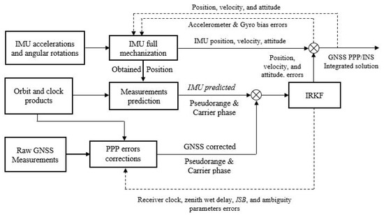
Figure 1.
Block diagram of tightly coupled GNSS PPP/INS integration.
4.1. System Model
The discrete form of the system model is given as [8]:
where is the predicted state error vector at epoch k; ; is the transition matrix; represents the system dynamic matrix; is the sampling interval; I is the identity matrix; is the estimated state error vector at epoch k − 1; is the noise coupling matrix; and refers to the system noise with Q covariance matrix. For the TC GNSS/INS integration, the state vector is given by:
where refer to the position errors; refer to the velocity errors; refer to the attitude angles errors; refer to the accelerometer bias errors; refer to the gyro bias errors; refer to the receiver clock error; refer to the wet zenith delay error; refer to the ISB error; and refer to the ambiguity parameter errors. The dynamic matrix can be adopted as in Equation (A1). The first-order Gauss Markov process is used to model the accelerometers and gyro bias as described in Equations (A10) and (A11) in Appendix A [10]. The noise coupling matrix G is in Equation (A12) in Appendix A [31,32]. In the prediction stage, the system transition matrix as in Equation (22) is used to predict the state vector δxk(−), and its a priori covariance matrix Pk(−) can be estimated as:
where Pk−1(+) is the state vector posteriori covariance matrix at epoch k − 1. It is worth mentioning that the a priori covariance matrix is assumed to be a diagonal matrix at the initial epoch. The Q matrix is diagonal, and it is set based on the system noise covariances with each state vector parameter. The system noise includes the accelerometer noise vector, gyro noise vector, Gaussian noise associated in the GM process of accelerometer bias, Gaussian noise associated in the GM process of gyro bias, driving noise for receiver clock error, driving noise for zenith wet delay error, and driving noise for ISB. The receiver clock error, zenith wet delay, and ISB are modeled as random walk processes. The stochastic parameters of both accelerometers and gyros provided in the IMU’s data sheets are used to construct the initial form of the process noise covariance matrix. However, Q requires further tuning to achieve the required performance for the application under consideration.
4.2. Measurements Model
The measurement model for the TC GNSS PPP/INS integration can be written as:
where is the observations noise with R covariance matrix; H is the coefficient matrix; and refers to the measurement error vector. The measurement error consists of the differences between the GPS, GLONASS, and Galileo IF linear combinations of carrier phase and pseudorange measurements and the predicted IMU-based counterparts, and can be written as:
The coefficient matrix for the TC GNSS PPP/INS integration can be constructed as:
where is an Nx3 matrix that contains a set of unit vectors ; N is the number of tracked satellites for each satellite’s system, namely NG, NR, and NE; is a 1 × 3 unit vector between the receiver and the corresponding satellite; and NG, NR, and NE refer to the GPS, GLONASS, and Galileo visible satellites. The matrix is multiplied by a transformation matrix [8] to convert the coordinate corrections from the ECEF frame to the curvilinear coordinate corrections . In the update stage, the Kalman gain K can be written as:
In the IRKF, an adaptive factor is adopted to balance the contribution of the predicted state vector and the robust estimation using the new measurements to compensate for the system model errors [33,34]. The adaptive factor can be determined as [35]:
where is the discrepancy in the predicted state; and are constants and can be set as ; ; and is the adaptive factor, which can take values in the range 0 to 1. can be determined as [35]:
where is the state vector estimate using the GNSS measurements at epoch k. As shown in Equation (29), the coefficient takes the value of 1 when the is less than , which indicates a good estimate of the predicted state vector. On the other hand, the coefficient takes the value of 0 when is higher than , which indicates that the contribution of the predicted state to the update stage has to be minimized, as shown in Equation (31). The values of and need to be further tuned to achieve the required performance for the application under consideration. In this study, the values of 1.5 and 4.5 are adopted for and , respectively. To control the predicted state contribution, a new formula of the Kalman gain is presented as:
It is worth mentioning that the measurement covariance matrix R is assumed to be a diagonal matrix. The diagonal elements are the variances of the IF linear combinations of the pseudorange measurements and carrier phase measurements , which are given by [36]:
where el refers to the elevation angle of the satellite; and ; f1 and f2 are GPS L1/L2 frequencies, GLONASS L1/L2 frequencies, and Galileo E1/E5a or E1/E5b frequencies; and and refer to the pseudorange and carrier phase standard deviations. In this study, two different GNSS receivers are used, namely Trimble R9s and u-blox F9P. The standard deviation of the carrier phase measurements is scaled by 100 times less than the pseudorange due to its high precision [37]. The adopted pseudorange and carrier phase standard deviations are 0.3 m and 0.003 m when the Trimble GNSS receiver is used. Due to the difference in the quality of the GNSS observations between the geodetic-grade and low-cost GNSS receivers, the adopted pseudorange and carrier phase standard deviations are 3 m and 0.03 m when the u-blox GNSS receiver is used. The a posteriori covariance matrix of the updated state vector can be estimated through [13]:
The innovation term dxk, which is used to update the predicted state vector, can be estimated as [10]:
In this study, we are using the closed-loop scheme, which means that δxk(−) = 0. Therefore, the innovation term can be re-written as:
In the IRKF, a modified covariance matrix for the GNSS measurements is introduced to compensate for the effect of measurement outliers. The modified measurement covariance matrix , which is assumed to be a diagonal matrix, is constructed for GPS, GLONASS, and Galileo pseudorange and carrier phase measurements as [38]:
The measurements’ residuals are firstly estimated to construct as:
The standardized residuals are then estimated as:
The standardized residuals are then used to determine the robust classification factor P for each specific measurement type individually. The classification factor for the ith number of measurements in the jth type of measurements can be estimated using the t-test statistics as [38]:
where is the t-test statistic for the ith measurement in the jth type as described in [38]; are the t-test critical values at significance levels, and is the degree of freedom for the jth measurement type; and is the number of jth type measurements. The significance levels need to be further tuned to achieve the required performance for the application under consideration. In this study, the values are adopted to be 0.15 and 0.01, respectively. The classification factor is then used to scale the variance of each measurement individually as:
where j refers to the observation type; i refers to the ith observation of the jth type. In this study, we have six types of measurements as described in Equation (37). Therefore, the j symbol takes values that range from one to six, and the i symbol depends on the number of the available measurements on each type. After this step, the GNSS measurements, including outliers, are down-weighted in the modified covariance matrix . The Kalman gain and a posteriori covariance matrix are then estimated as follows:
Finally, the updated state vector is estimated as:
In the closed-loop scheme, Equation (44) can be simplified as:
The updated state vector parameters are used to correct the IMU full mechanization outputs, resulting in the TC GNSS PPP/INS integrated solution.
5. Experimental Setup
5.1. GNSS Receiver and IMUs
In this study, three GNSS receivers were used. The first is the u-blox F9P GNSS receiver, while the second is the Trimble R9s geodetic receiver. The used GNSS measurements from both receivers are summarized in Section 2. As mentioned earlier, the BeiDou measurements were excluded in this study due to the low number of tracked BeiDou satellites (two or less) during the field trials. The third one is the NovAtel PwrPak7 geodetic receiver, which was used to generate the reference solutions. Two IMUs were used in the field trials, namely the Stim300 tactical-grade IMU and the xsens MTi 670 IMU industrial-grade. The specifications of both IMUs are summarized in Table 2.
Table 2.
IMUs’ specifications.
5.2. Reference Solutions
The NovAtel PwrPak7 GNSS receiver and the Stim300 were used to generate the reference solutions for the three field trials. The raw GNSS measurements from PwrPak7 and the raw measurements from Stim300 were utilized along with GNSS measurements from a base station to generate a TC carrier phase-based differential GNSS (DGNSS)/INS integrated solution for each field trial. The TC DGNSS/INS solution was generated in post-processing mode using NovAtel’s waypoint inertial explorer (IE) software. Three virtual reference stations (VRS) were constructed using Cansel’s GNSS permanent network (CAN-NET) in the Toronto area to provide raw GNSS measurements, which were used to generate the reference solutions for the three field trials.
5.3. Processing Scheme
To thoroughly evaluate the performance of the proposed integrated system, four different TC GNSS PPP/INS integrated solutions were developed as follows:
Ublox–Xsens: The u-blox GPS, GLONASS, and Galileo measurements were tightly-coupled integrated with the xsens MTi670 accelerometers and gyro measurements. This represents the main system that was developed in this study to provide an ultra-low-cost integrated solution.
Trimble–Xsens: In this solution, Trimble GNSS measurements and xsens MTi670 accelerations and angular rotation measurements were integrated in a tightly-coupled mode. This system examined the performance of the integrated system when an industrial-grade IMU is used.
Ublox–Stim: This solution took advantage of the tactical grade of the Stim300 to provide better accuracy, especially for the attitude solution.
Trimble–Stim: This system was adopted in this study to provide the most precise autonomous positioning and attitude solution. The performance of the above systems was assessed in comparison with the Trimble–Stim system.
It should be pointed out that the lever arm between each GNSS antenna and the corresponding IMU is precisely measured and compensated for during the processing process. It should be pointed that cost of the Ublox–Xsens system is at least 10 times lower than the Trimble–Stim system.
5.4. Sensors Setup
All sensors were rigidly fixed on a wooden panel and firmly mounted on the vehicle’s rooftop, as shown in Figure 2. The u-blox F9P GNSS receiver was connected to a u-blox patch antenna, the Trimble GNSS receiver was connected to Trimble Zephyr 3 antenna, and the PwrPak7 was connected to an OmniStar antenna. The axes of both IMUs were aligned with the vehicle’s body frame axes, in which the y-axis refers to the forward direction, the x-axis is the transversal direction, and the z-axis is completing a right-handed system.
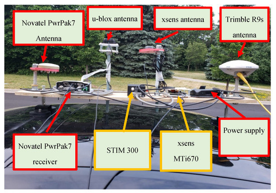
Figure 2.
Sensors set up on vehicle’s rooftop.
6. Result Analysis
Three land vehicular field trials were conduct ed in Toronto, Canada, to assess the performance of the proposed ultra-low-cost TC triple-constellation GNSS PPP/INS integrated system. The first field trial aimed to assess the positioning solution in a suburban area under both an open-sky environment and a partial GNSS outage. Both of the second and the third field trials were carried out in combined suburban and urban areas, where the GNSS signals were partially or fully blocked.
6.1. First Field Trial
The field trial was on 22 June 2020 and lasted for about 30 min. Figure 3 shows the full trajectory of the field trial. As shown in Figure 4, the number of tracked GPS, GLONASS, and Galileo satellites ranges from 4 to 13 when the u-blox GNSS receiver is used, while the number of tracked satellites ranges from 9 to 16 when the Trimble GNSS receiver is used. The reason for the low number of tracked satellites for the u-blox receiver is that the u-blox supports only civil signals, L1 C/A and L2C, for GPS constellation. Unfortunately, however, the L2C signals are only transmitted by modernized GPS satellites. This means that fewer GPS dual-frequency measurements were available at the time of data collection to form the conventional IF linear combination. The tracking capability of the u-blox GNSS receiver significantly affects the accuracy of the positioning solution, as shown in Figure 5, Figure 6 and Figure 7, compared to the Trimble GNSS receiver counterpart. It should be pointed out that both the Trimble–Xsense and Trimble–Stim solutions show similar positioning performance. Additionally, as can be seen, the quality of the IMU grade affects the positioning solution due to the high variability of the number of tracked satellites when the u-blox receiver is used. The Ublox–Stim solution smoothed most of the jumps that are present during the epochs when a low number of satellites are tracked, compared to the Ublox–Xsens solution. The Trimble-based positioning solution outperforms the u-blox-based counterpart, proving that the GNSS receiver tracking capability is the dominant factor for the accuracy of the positioning solution. Additionally, both of the Trimble–Xsens and Trimble–Stim solutions show similar positioning performance.
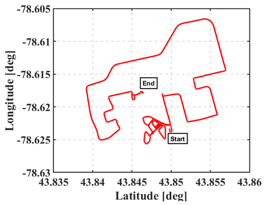
Figure 3.
The trajectory of the first vehicular test, Toronto, Ontario, Canada (22 June 2020).
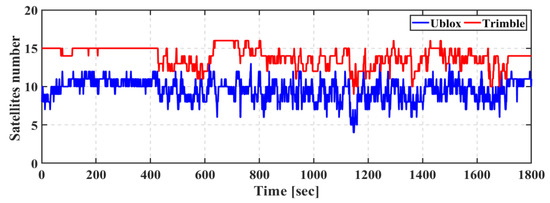
Figure 4.
First field trial: Number of tracked GPS, GLONASS, and Galileo satellites.
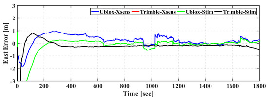
Figure 5.
First field trial: East positioning error of real-time TC GNSS PPP/INS for Ublox–Xsens, Trimble–Xsens, Ublox–Stim, and Trimble–Stim solutions.
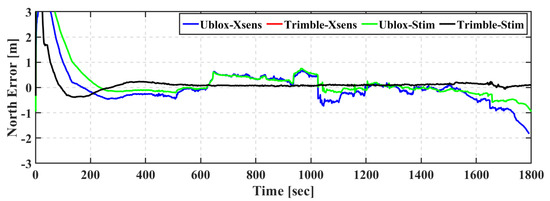
Figure 6.
First field trial: North positioning error of real-time TC GNSS PPP/INS for Ublox–Xsens, Trimble–Xsens, Ublox–Stim, and Trimble–Stim solutions.
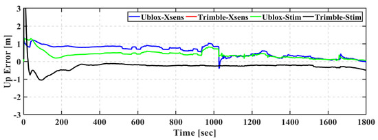
Figure 7.
First field trial: Up positioning error of real-time TC GNSS PPP/INS for Ublox–Xsens, Trimble–Xsens, Ublox–Stim, and Trimble–Stim solutions.
Table 3 shows the root-mean-square (RMS) of positioning errors of the Ublox–Xsens, Trimble–Xsens, Ublox–Stim, and Trimble–Stim integrated solutions in the east, north, and up directions. It should be pointed out that the first three minutes, which represent the solution convergence, are excluded from the results. As can be seen, the quality of the IMU grade is the dominant factor that degrades the positioning accuracy for the u-blox-based solutions. The Ublox–Xsens solution achieves sub-meter positioning accuracy in all directions. On the other hand, the positioning accuracy is improved to reach decimeter-level in the east, north, and up directions when the Stim300 is utilized with the u-blox F9P GNSS receiver. This represents an improvement of 15%, 59%, and 58% in the east, north, and up directions, respectively. The Trimble-based solutions achieve better positioning accuracy compared to the u-blox-based counterparts. The RMS of the Trimble–Xsens solution is 0.221 m, 0.118 m, and 0.261 m in the east, north, and up directions, respectively, compared to 0.531 m, 0.799 m, and 0.652 m for the Ublox–Xsens solution. Additionally, the RMS of the Trimble–Stim solution is 0.222 m, 0.117 m, and 0.261 m in the east, north, and up directions, respectively, compared to 0.449 m, 0.325 m, and 0.270 m for the Ublox–Stim solution. Moreover, both of the Trimble–Xsens and Trimble–Stim solutions show similar positioning accuracy, which aligns with the error series in Figure 5, Figure 6 and Figure 7.
Table 3.
RMS error and mean error (m) in east, north, and up directions—first field trial.
Figure 8 shows the attitude errors for the pitch, roll, and azimuth angles of the xsens-based integrated solutions, while attitude errors of the Stim-based integrated solutions are presented in Figure 9. It can be seen that the attitude solution performance is significantly improved when the Stim300 is used, regardless of whether the Trimble or u-blox GNSS receiver is used.
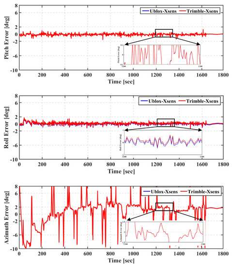
Figure 8.
First field trial: Pitch (top), roll (middle), and azimuth (bottom) of real-time TC GNSS PPP/INS for Ublox–Xsens and Trimble–Xsens solutions.
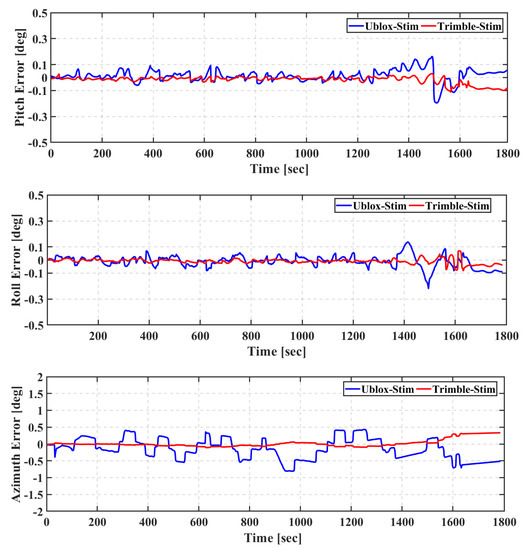
Figure 9.
First field trial: Pitch (top), roll (middle), and azimuth (bottom) of real-time TC GNSS PPP/INS for Ublox–Stim and Trimble–Stim solutions.
The RMS and the mean of the attitude errors of the Ublox–Xsens, Trimble–Xsens, Ublox–Stim, and Trimble–Stim integrated solutions are presented in Table 4. The RMS of the attitude errors of the Ublox–Xsens solution is 0.293°, 0.331°, and 3.470° for pitch, roll, and azimuth, respectively, compared to 0.292°, 0.363°, and 3.475°, respectively, for the Trimble–Xsens solution. As can be seen in Table 4, the IMU grade is the dominant factor that affects the attitude solution accuracy, regardless of whether a geodetic or low-cost GNSS receiver is used. For example, the RMS of the attitude errors of the Ublox–Stim is improved by 83%, 86%, and 90% for pitch, roll, and azimuth angles, respectively, in comparison with the Ublox–Xsens solution. The same improvement in the attitude solution accuracy is achieved when the Stim300 is utilized with the Trimble GNSS receiver instead of the xsens MTi670.
Table 4.
RMS error and mean error (deg) of roll, pitch, and azimuth angles—first field trial.
6.2. Second Field Trial
The second field trial was conducted in an urban area with a challenging environment. The trial lasted for about 45 min, and the full trajectory is shown in Figure 10. The number of the tracked satellites ranged from 1 to 17 when the u-blox GNSS receiver was used, while the number of the tracked satellites ranged from 7 to 19 when the Trimble GNSS receiver was used, as shown in Figure 11.
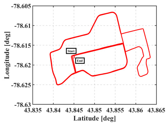
Figure 10.
The trajectory of the second vehicular test, Toronto, Ontario, Canada (22 June 2020).
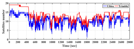
Figure 11.
Second field trial: Number of tracked GPS, GLONASS, and Galileo satellites.
As shown in Figure 12, Figure 13 and Figure 14, the Ublox–Stim and Ublox–Xsens solutions show comparable performance in the east, north, and up directions. However, the Ublox–Stim solution smoothed most of the jumps that are present during the epochs when a low number of satellites are tracked, while there are some jumps lower than one meter for the Ublox–Xsens solution. The Trimble-based positioning solutions outperform the u-blox-based solutions, which is mainly due to the lower tracking capability of the u-blox receiver. Additionally, both of the Trimble–Xsens and Trimble–Stim solutions show similar performance with the superiority of the Trimble–Stim solution in the convergence performance.
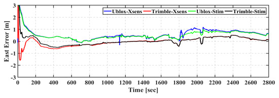
Figure 12.
Second field trial: East positioning error of real-time TC GNSS PPP/INS for Ublox–Xsens, Trimble–Xsens, Ublox–Stim, and Trimble–Stim solutions.
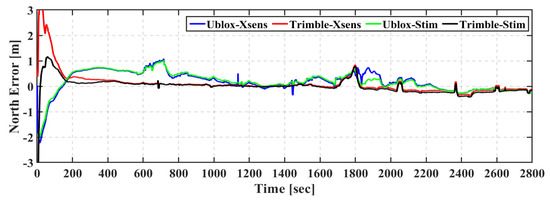
Figure 13.
Second field trial: East positioning error of real-time TC GNSS PPP/INS for Ublox–Xsens, Trimble–Xsens, Ublox–Stim, and Trimble–Stim solutions.
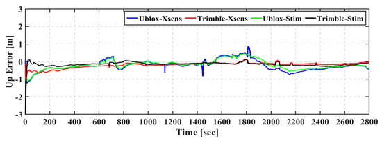
Figure 14.
Second field trial: East positioning error of real-time TC GNSS PPP/INS for Ublox–Xsens, Trimble–Xsens, Ublox–Stim, and Trimble–Stim solutions.
Table 5 shows the root-mean-square (RMS) of positioning errors of the Ublox–Xsens, Trimble–Xsens, Ublox–Stim, and Trimble–Stim integrated solutions in the east, north, and up directions. It should be pointed out that the first three minutes, which represent the solution convergence, are excluded from the RMS values. The Ublox–Xsens solution achieves meter-level positioning accuracy in the east direction and sub-meter-level positioning accuracy in the north and up directions, compared to sub-meter-level positioning accuracy in the east, north, and up directions for the Ublox–Stim solution. The Trimble-based solutions achieve better positioning accuracy compared to the u-blox-based counterparts, which agree with the findings of the first trial. The RMS values of the Trimble–Xsens solution are 0.354 m, 0.486 m, and 0.250 m in the east, north, and up directions, respectively, compared to 1.200 m, 0.713 m, and 0.665 m for the Ublox–Xsens solution. Additionally, the RMS values of the Trimble–Stim solution are 0.254 m, 0.175 m, and 0.150 m in the east, north, and up directions, respectively, compared to 1.050 m, 0.699 m, and 0.539 m for the Ublox–Stim solution. Moreover, both of the Trimble–Xsens and Trimble–Stim positioning solutions achieve decimeter-level positioning accuracy in the east, north, and up directions.
Table 5.
RMS error and mean error (m) in east, north, and up directions—first field trial.
Figure 15 shows the attitude errors for the pitch, roll, and azimuth angles of the Xsens-based integrated solutions, while the attitude errors of the Stim-based solutions are presented in Figure 16.
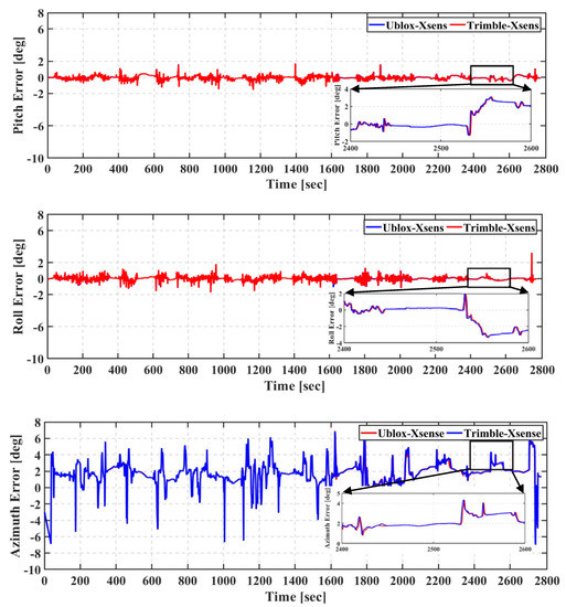
Figure 15.
Second field trial: Pitch (top), roll (middle), and azimuth (bottom) of real-time TC GNSS PPP/INS for Ublox–Xsens and Trimble–Xsens solutions.
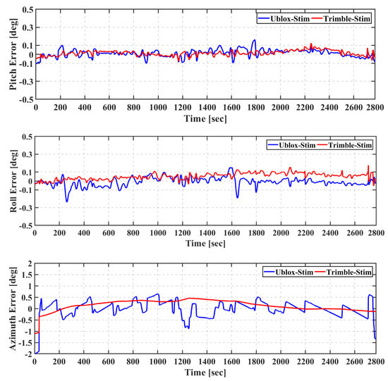
Figure 16.
Second field trial: Pitch (top), roll (middle), and azimuth (bottom) of real-time TC GNSS PPP/INS for Ublox–Stim and Trimble–Stim solutions.
For the Trimble–Xsens and Ublox–Xsens solutions, the error in the pitch and roll angles is typically less than 2°, while it reaches 6° for the azimuth. It can be seen that the attitude solution is significantly improved when the Stim300 is used, regardless of whether the Trimble or u-blox GNSS receiver is used. For both of the Trimble–Stim and Ublox–Stim solutions, the error in the pitch and roll angles is typically less than 0.1°, while it reaches 0.5° for the azimuth.
The RMS and the mean of the attitude errors of Ublox–Xsens, Trimble–Xsens, Ublox–Stim, and Trimble–Stim integrated solutions are presented in Table 6. The RMS values of the attitude errors of the Ublox–Xsens solution are 1.623°, 1.732°, and 2.254° for the pitch, roll, and azimuth, respectively, compared to 1.626°, 1.730°, and 2.270°, respectively, for the Trimble–Xsens solution. It can be seen that the IMU grade is the dominant factor that affects the accuracy of the attitude solution, regardless of whether a geodetic or a low-cost GNSS receiver is used, as concluded from the results of the first trial. For example, the RMS values of the attitude errors of the Ublox–Xsens solution are improved from 1.623°, 1.732°, and 2.254° for pitch, roll, and azimuth angles, respectively, to 0.043°, 0.051°, and 0.373° for the Ublox–Stim solution. The attitude accuracy is improved by 97%, 96%, and 87% for the pitch, roll, and azimuth angles, respectively, when the Stim300 is used with the Trimble GNSS receiver instead of the xsens MTi670.
Table 6.
RMS error and mean error (deg) of roll, pitch, and azimuth angles—second field trial.
6.3. Third Field Trial
The third field trial was conducted in a combined urban and suburban area with a challenging environment that included tall buildings and urban foliage (about 3 m). The trial lasted for about 34 min and the full trajectory of the field trial is shown in Figure 17. The number of tracked satellites ranged from 0 to 19 when the u-blox GNSS receiver was used, while the number of tracked satellites ranged from 4 to 19 when the Trimble GNSS receiver was used, as shown in Figure 18.
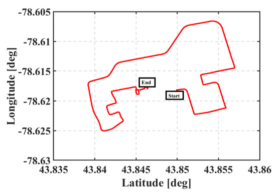
Figure 17.
The trajectory of the third vehicular test, Toronto, Ontario, Canada (22 June 2020).
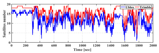
Figure 18.
Third field trial: Number of tracked GPS, GLONASS, and Galileo satellites.
As shown in Figure 19, Figure 20 and Figure 21, the Ublox–Stim solution shows better performance than the Ublox–Xsens solution, especially in the east direction. Additionally, the Ublox–Stim solution smoothed the majority of the jumps that are present during the epochs when a low number of satellites are tracked, while some jumps reach more than a meter for the Ublox–Xsens solution. It is worth mentioning that at some points in time, the positioning errors in the east and north directions of both of the Ublox–Xsens and Ublox–Stim solutions exceed one meter, which is mainly due to the high variability of the tracked satellites. The Trimble-based positioning solutions outperform the u-blox-based solutions, which is mainly due to the tracking capability of the GNSS receiver.
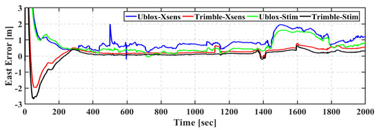
Figure 19.
Third field trial: East positioning error of real-time TC GNSS PPP/INS for Ublox–Xsens, Trimble–Xsens, Ublox–Stim, and Trimble–Stim solutions.
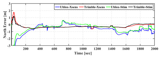
Figure 20.
Third field trial: East positioning error of real-time TC GNSS PPP/INS for Ublox–Xsens, Trimble–Xsens, Ublox–Stim, and Trimble–Stim solutions.
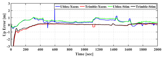
Figure 21.
Third field trial: East positioning error of real-time TC GNSS PPP/INS for Ublox–Xsens, Trimble–Xsens, Ublox–Stim, and Trimble–Stim solutions.
The root-mean-square (RMS) and mean of positioning errors of the Ublox–Xsens, Trimble–Xsens, Ublox–Stim, and Trimble–Stim integrated solutions in the east, north, and up directions are presented in Table 7. The RMS values of the Ublox–Xsens positioning solution are 1.029 m, 0.687 m, and 0.466 m in the east, north, and up directions, respectively. Due to the high variability of the tracked satellites when the u-blox GNSS receiver is used, the Ublox–Stim solution shows better positioning performance than the Ublox–Xsens counterpart. The Ublox–Xsens solution is improved by 27%, 18%, and 21% in the east, north, and up directions, respectively, when the Stim300 IMU is used with the u-blox F9P GNSS receiver. As concluded from the first two field trials, the Trimble-based solutions achieve better positioning accuracy than the u-blox-based counterparts. The RMS errors of the Ublox–Xsens positioning solution are improved from 1.029 m, 0.687 m, and 0.466 m in the east, north, and up directions, respectively, to 0.362 m, 0.300 m, and 0.102 m for the Trimble–Xsens solution. Additionally, the RMS errors of the Ublox–Stim positioning solution are improved from 0.749 m, 0.562 m, and 0.565 m in the east, north, and up directions, respectively, to 0.212 m, 0.289 m, and 0.132 m for the Trimble–Stim.
Table 7.
RMS error and mean error (m) in east, north, and up directions—third field trial.
Figure 22 shows the attitude errors for the Xsens-based integrated solutions, while the attitude errors for the Stim-based solutions are presented in Figure 23.
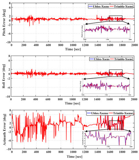
Figure 22.
Third field trial: Pitch (top), roll (middle), and azimuth (bottom) of real-time TC GNSS PPP/INS for Ublox–Xsens and Trimble–Xsens solutions.
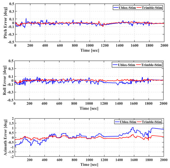
Figure 23.
Third field trial: Pitch (top), roll (middle), and azimuth (bottom) of real-time TC GNSS PPP/INS for Ublox–Stim and Trimble–Stim solutions.
The attitude errors of both of the Trimble–Xsens and Ublox–Xsens solutions are less than 2° for the pitch and roll components and less than 6° for the azimuth. It can be seen that for both of the Trimble–Stim and Ublox–Stim solutions, the attitude errors are less than 0.1° for the pitch and roll components and less than 0.5° for the azimuth. However, at some points in time, the azimuth angle errors for the Ublox–Stim solution exceed 0.5°, which is mainly due to the degradation in the positioning accuracy.
The RMS and the mean of the attitude errors of Ublox–Xsens, Trimble–Xsens, Ublox–Stim, and Trimble–Stim integrated solutions are presented in Table 8. The RMS values of the attitude errors of the Ublox–Xsens solution are 0.719°, 0.334°, and 2.980° for the pitch, roll, and azimuth, respectively, compared to 0.718°, 0.335°, and 2.985°, respectively, for the Trimble–Xsens solution. As concluded from the first two field trials, the IMU grade is the dominant factor that affects the attitude solution accuracy, regardless of whether a geodetic or low-cost GNSS receiver is used. For example, the RMS values of the attitude errors of the Ublox–Xsens are improved from 0.719°, 0.334°, and 2.980° for the pitch, roll, and azimuth angles, respectively, to 0.034°, 0.047°, and 0.466° for the Ublox–Stim solution. Additionally, the attitude accuracy for the Trimble–Xsens solution is improved by 97%, 95%, and 96% for the pitch, roll, and azimuth angles, respectively, compared to the Trimble–Stim solution.
Table 8.
RMS error and mean error (deg) of roll, pitch, and azimuth angles—third field trial.
7. Conclusions
In this study, an ultra-low-cost TC triple-constellation GNSS PPP/INS integrated system was developed. The developed system tightly integrates data from the newly developed low-cost dual-frequency u-blox F9P GNSS receiver and the industrial-grade xsens MTi670 IMU. The performance of the developed system was assessed through three land vehicular field trials. The first field trial was carried out to assess the integrated solution in an open-sky environment, while the second and third field trials were carried out to assess the integrated solution under challenging environments. It was shown that the proposed Ublox–Xsens system achieved sub-meter-level PPP accuracy in an open-sky environment, while it achieved meter-level PPP accuracy in challenging environments. The relatively low PPP accuracy is due mainly to the tracking capability of the u-blox F9P GNSS receiver, which led to tracking a limited number of GPS satellites at the time of observations. The average RMS of the attitude errors of the integrated solution was 0.878°, 0.799°, and 2.901° for the pitch, roll, and azimuth angles, respectively. The positioning accuracy of the integrated solution showed a significant improvement when the Trimble R9s geodetic receiver was used along with the xsens MTi670 IMU. The positioning solution of the Trimble–Xsens integrated system consistently achieved decimeter-level positioning accuracy under both open-sky and challenging environments. The Ublox–Stim integrated system, in which the u-blox F9P GNSS receiver and Stim300 tactical-grade IMU were used, achieved comparable positioning accuracy to the Ublox–Xsens solution. In contrast to the Ublox–Xsens solution, however, the Ublox–Stim integration smoothed the majority of the jumps that were present in the positioning solution during the epochs when a low number of satellites were tracked. Moreover, the accuracy of the obtained attitude solution was significantly improved when the Stim300 IMU was used. The average RMS of the attitude errors of the Ublox–Stim solution was 0.042°, 0.048°, and 0.394° for the pitch, roll, and azimuth angles, respectively. The Trimble–Stim integrated system showed the best positioning and attitude solution accuracy. However, the relatively high cost of the Trimble–Stim integrated system might limit its usage for a wide range of applications.
Author Contributions
A.E. and A.E.-R. conceived the idea and wrote the paper. A.E. implemented the experimental tests and assessed them under the supervision of A.E.-R. Both authors have read and agreed to the published version of the manuscript.
Funding
This research received no external funding.
Institutional Review Board Statement
Not Applicable.
Informed Consent Statement
Not applicable.
Data Availability Statement
Data sharing is not applicable to this article.
Acknowledgments
This research is supported by the Government of Ontario and Ryerson University through the Ontario Trillium Scholarship. The authors would like to thank NovAtel for providing the Waypoint Inertial Explorer (IE) software and Cansel for providing the VRS GNSS measurements. Additionally, the authors would like to thank the CNES Analysis Center for making the real-time GNSS orbit and clock products available. The first author would like to extend his thanks to the research team at Ryerson University for the help in the data collection.
Conflicts of Interest
The authors declare no conflict of interest.
Appendix A
The dynamic matrix F can be adopted as:
where the elements of the F matrix can be written as follows:
The first-order Gauss Markov (GM) process is used to model the accelerometers and gyro bias. It can be presented in a matrix format as [10]:
where β refers to the reciprocal of the correlation time for accelerometer and gyro biases. The noise coupling matrix G is adopted as [31,32]:
The elements of the G matrix can be adopted as:
where are the variances of the white noise associated with the first-order GM process for accelerometer and gyro biases, respectively.
References
- Zumberge, J.; Heflin, M.; Jefferson, D.; Watkins, M.; Webb, F. Precise point positioning for the efficient and robust analysis of GPS data from large networks. J. Geophys. Res. Solid Earth 1997, 102, 5005–5017. [Google Scholar] [CrossRef]
- Robustelli, U.; Baiocchi, V.; Marconi, L.; Radicioni, F.; Pugliano, G. Precise Point Positioning with single and dual-frequency multi-GNSS Android smartphones. In Proceedings of the CEUR Workshop Proceeding, Vienna, Austria, 3–6 November 2020. [Google Scholar]
- Elmezayen, A.; El-Rabbany, A. Precise point positioning using world’s first dual-frequency GPS/GALILEO smartphone. Sensors 2019, 19, 2593. [Google Scholar] [CrossRef] [PubMed]
- Psychas, D.; Bruno, J.; Massarweh, L.; Darugna, F. Towards sub-meter positioning using Android raw GNSS measurements. In Proceedings of the 32nd International Technical Meeting of the Satellite Division of The Institute of Navigation (ION GNSS+ 2019), Miami, FL, USA, 16–20 September 2019. [Google Scholar]
- Wu, Q.; Sun, M.; Zhou, C.; Zhang, P. Precise point positioning using dual-frequency GNSS observations on smartphone. Sensors 2019, 19, 2189. [Google Scholar] [CrossRef]
- u-blox. ZED-F9P Module. Available online: https://www.u-blox.com/en/product/zed-f9p-module (accessed on 1 March 2021).
- Hoffman-Wellenhof, B.; Lichtenegger, H.; Wasle, E. GNSS-Global Navigation Satellite Systems.GPS, GLONASS, Galileo and More; Springer: Wien, Austria, 2008. [Google Scholar]
- Noureldin, A.; Karamat, T.B.; Georgy, J. Fundamentals of Inertial Navigation, Satellite-Based Positioning and Their Integration; Springer Science & Business Media: Berlin/Heidelberg, Germany, 2012. [Google Scholar]
- Du, S.; Gao, Y. Integration of PPP GPS and low cost IMU. In Proceedings of the Canadian Geomatics Conference, Calgary, AB, Canada, 15–18 June 2010. [Google Scholar]
- Abd Rabbou, M.; El-Rabbany, A. Tightly coupled integration of GPS precise point positioning and MEMS-based inertial systems. GPS Solut. 2015, 19, 601–609. [Google Scholar] [CrossRef]
- Gao, G.; Lachapelle, G. A novel architecture for ultra-tight HSGPS-INS integration. Positioning 2008, 1, 46–61. [Google Scholar] [CrossRef]
- Falco, G.; Pini, M.; Marucco, G. Loose and tight GNSS/INS integrations: Comparison of performance assessed in real urban scenarios. Sensors 2017, 17, 255. [Google Scholar] [CrossRef] [PubMed]
- Gao, Z.; Zhang, H.; Ge, M.; Niu, X.; Shen, W.; Wickert, J.; Schuh, H. Tightly coupled integration of multi-GNSS PPP and MEMS inertial measurement unit data. GPS Solut. 2017, 21, 377–391. [Google Scholar] [CrossRef]
- Wang, D.; Dong, Y.; Li, Z.; Li, Q.; Wu, J. Constrained MEMS-based GNSS/INS tightly-coupled system with robust Kalman filter for accurate land vehicular navigation. IEEE Trans. Instrum. Meas. 2019. [Google Scholar] [CrossRef]
- Liu, S.; Sun, F.; Zhang, L.; Li, W.; Zhu, X. Tight integration of ambiguity-fixed PPP and INS: Model description and initial results. GPS Solut. 2016, 20, 39–49. [Google Scholar] [CrossRef]
- Huang, A. A Tutorial on Bayesian Estimation and Tracking Techniques Applicable to Non-Linear and Non-Gaussian Process; MITRE Corporation: McLean, VA, USA, 2005. [Google Scholar]
- Abd Rabbou, M.; El-Rabbany, A. Integration of GPS precise point positioning and MEMS-based INS using unscented particle filter. Sensors 2015, 15, 7228–7245. [Google Scholar] [CrossRef]
- Georgy, J.; Iqbal, U.; Bayoumi, M.; Noureldin, A. Reduced inertial sensor system (RISS)/GPS integration using particle filtering for land vehicles. In Proceedings of the 21st International Technical Meeting of the Satellite Division of the Institute of Navigation (ION GNSS 2008), Savannah, GA, USA, 16–19 September 2008. [Google Scholar]
- Elsheikh, M.; Abdelfatah, W.; Noureldin, A.; Iqbal, U.; Korenberg, M. Low-Cost Real-Time PPP/INS Integration for Automated Land Vehicles. Sensors 2019, 19, 4896. [Google Scholar] [CrossRef]
- Elsheikh, M.; Noureldin, A.; Korenberg, M. Integration of GNSS Precise Point Positioning and Reduced Inertial Sensor System for Lane-Level Car Navigation. IEEE Trans. Intell. Transp. Syst. 2020. [Google Scholar] [CrossRef]
- Nie, Z.; Liu, F.; Gao, Y. Real-time precise point positioning with a low-cost dual-frequency GNSS device. GPS Solut. 2020, 24, 9. [Google Scholar] [CrossRef]
- Kouba, J.; Héroux, P. Precise point positioning using IGS orbit and clock products. GPS Solut. 2001, 5, 12–28. [Google Scholar] [CrossRef]
- Montenbruck, O.; Steigenberger, P.; Prange, L.; Deng, Z.; Zhao, Q.; Perosanz, F.; Romero, I.; Noll, C.; Stürze, A.; Weber, G. The Multi-GNSS Experiment (MGEX) of the International GNSS Service (IGS)–achievements, prospects and challenges. Adv. Space Res. 2017, 59, 1671–1697. [Google Scholar] [CrossRef]
- Montenbruck, O.; Hauschild, A. Code biases in multi-GNSS point positioning. In Proceedings of the 2013 International Technical Meeting of The Institute of Navigation, San Diego, CA, USA, 28–30 January 2013. [Google Scholar]
- Steigenberger, P.; Hugentobler, U.; Loyer, S.; Perosanz, F.; Prange, L.; Dach, R.; Uhlemann, M.; Gendt, G.; Montenbruck, O. Galileo orbit and clock quality of the IGS Multi-GNSS Experiment. Adv. Space Res. 2015, 55, 269–281. [Google Scholar] [CrossRef]
- Saastamoinen, J. Contributions to the theory of atmospheric refraction. Bull. Géod. 1972, 105, 279–298. [Google Scholar] [CrossRef]
- Böhm, J.; Möller, G.; Schindelegger, M.; Pain, G.; Weber, R. Development of an improved empirical model for slant delays in the troposphere (GPT2w). GPS Solut. 2015, 19, 433–441. [Google Scholar] [CrossRef]
- Kouba, J. A Guide to Using International GNSS Service (IGS) Products. IGS [Online]. 2015. Available online: https://kb.igs.org/hc/en-us/articles/201271873-A-Guide-to-Using-the-IGS-Products (accessed on 25 December 2019).
- Farrell, J. Aided Navigation: GPS with High Rate Sensors; McGraw-Hill, Inc.: New York, NY, USA, 2008. [Google Scholar]
- Du, S. Integration of Precise Point Positioning and Low Cost MEMS IMU; University of Calgary: Calgary, AB, Canada, 2010. [Google Scholar]
- Gao, Y.; Liu, S.; Atia, M.M.; Noureldin, A. INS/GPS/LiDAR integrated navigation system for urban and indoor environments using hybrid scan matching algorithm. Sensors 2015, 15, 23286–23302. [Google Scholar] [CrossRef] [PubMed]
- Abd Rabbou, M.; El-Rabbany, A. Precise point positioning using multi-constellation GNSS observations for kinematic applications. J. Appl. Geod. 2015, 9, 15–26. [Google Scholar] [CrossRef]
- Yang, Y.; He, H.; Xu, G. Adaptively robust filtering for kinematic geodetic positioning. J. Geod. 2001, 75, 109–116. [Google Scholar] [CrossRef]
- Yang, Y.; Song, L.; Xu, T. Robust estimator for correlated observations based on bifactor equivalent weights. J. Geod. 2002, 76, 353–358. [Google Scholar] [CrossRef]
- Xu, G.; Xu, Y. GPS: Theory, Algorithms and Applications; Springer: Berlin/Heidelberg, Germany, 2016. [Google Scholar]
- Cai, C.; Gao, Y. Modeling and assessment of combined GPS/GLONASS precise point positioning. GPS Solut. 2013, 17, 223–236. [Google Scholar] [CrossRef]
- De Bakker, P.F.; Tiberius, C.C. Real-time multi-GNSS single-frequency precise point positioning. GPS Solut. 2017, 21, 1791–1803. [Google Scholar] [CrossRef]
- Zhang, Q.; Zhao, L.; Zhao, L.; Zhou, J. An improved robust adaptive Kalman filter for GNSS precise point positioning. IEEE Sens. J. 2018, 18, 4176–4186. [Google Scholar] [CrossRef]
Publisher’s Note: MDPI stays neutral with regard to jurisdictional claims in published maps and institutional affiliations. |
© 2021 by the authors. Licensee MDPI, Basel, Switzerland. This article is an open access article distributed under the terms and conditions of the Creative Commons Attribution (CC BY) license (https://creativecommons.org/licenses/by/4.0/).