Bathymetric Survey for Enhancing the Volumetric Capacity of Tagwai Dam in Nigeria via Leapfrogging Approach

Abstract

From a global perspective, dams are constructed to trap water flowing from a higher concentration to a lower concentration into a basin for several purposes to aid humanity. The continuous monitoring of dams is prudent for measuring the rate of sedimentation and siltation, and to ensure that it functions to its full capacity. The Tagwai dam is used for irrigation and domestic activities. It was observed that there is a shortage in its storage capacity and supplies due to sedimentation, and coupled with this is the fact that the majority of the communities are not connected to the tap water system; if not, the problem would have been evidently pronounced. However, to determine the present volume of water and provide possible ways of increasing the reservoir’s storage capacity, the leapfrogging approach was used to improve the basin. The data were collected using a single beam echosounder and Hi-Target V30 differential global positioning system (DGPS). The sounder was used to acquire bathymetric data, while the DGPS was used to delineate the shoreline. The data were interpolated using the ordinary Kriging technique. After that, the leapfrogging method was grouped into four scenarios: Scenario A, B, C, and D. In each stage, the volume was computed using Simpson’s 3/8 integrated model. Scenario A is the present stage of the reservoir. Consequently, the results show that, while scenario B and C presented an appreciable increase in volume at the instant, scenario D illustrated a tremendous improvement in the storage capacity, and it is a win-win situation. The decision on which leapfrogging approach to employ depends on the government’s willingness to enhance the reservoir’s capacity and the resources available, such as human and financial capital to execute the project.

1. Introduction

All over the world, dams are built to impound water for several purposes and to enhance developmental activities at different capacities [1,2,3]. Monitoring these dams is essential due to the negative effects of sedimentation and siltation on the storage capacity of any reservoir [4]. This menace, caused by sediment from the catchment area being trapped as a result of the constructed embarkment around the dam, “is most notably at the dam axis” [5,6]. Investigating the amount of deposited sediment or the reservoir capacity at any moment is only possible through a bathymetric survey, and a coinciding delineation of the shoreline, at the time of the survey [7,8]. The bulk of this material reduces the volumetric content, thereby causing a shortage of supplies [9]. Additionally, determining sedimentation distribution as it affects dam bed configuration and the number of deposited materials is achievable via bathymetric observation [2]. Bathymetric observation carried out using a single-beam echo sounder is deficient of footprints; therefore, the data acquired need inference in order to account for the sparse area [10]. If the interpolator components are selected well, the estimated output will be reliable, but will not fit as precisely as its counterpart obtained using a multibeam echosounder [11]. However, the estimated output can be used to compute the reservoir storage capacity, and the rate of sediment can also be determined via cut and fill for reference purposes [12].

However, leapfrogging is the process of establishing new positions by tracking and orienting existing known positions [13]. It is a concept in which past and present spatial information technology is used to innovate a radical geospatial system [14,15], taking advantage of existing procedures to grow the economy rapidly by skipping some development stages [16]. In addition, leapfrogging is cost implicative, but this cannot be compared with its overall benefits [17,18]. Consequently, Tagwai dam serves as the only water storage system in Minna metropolis, Niger State, Nigeria. The reservoir supplies water to Minna metropolis for domestic and other uses. It also serves for irrigation purposes. The dam was constructed in the year 1978 to meet the needs of only small communities. However, with population growth and development, the storage system experienced shortages, mostly in the dry season. Moreover, not all communities are connected to tap water. If 70% of all the households were connected to potable water, the shortage would have been pronounced. Thus, the government is considering increasing the dam storage capacity, thereby improving the economic benefits. Hence, the objective of this paper is to model the lake floor at present and to provide a possible way of increasing the volumetric capacity of the dam through the leapfrogging approach. In addition, accurate determination and modelling of the seafloor levels are essential to avoid unnecessary over-dredging and extra costs. The ordinary Kriging technique was used to interpolate the single beam echo sounder data because it supports the Digital Depth Model (DDM). This is because DDM describes the variability of the distance between the sea surface and sea bottom [19]. However, other interpolation techniques are adequate for sparse date estimation [20] and the correct method to adopt depends on the analyst.

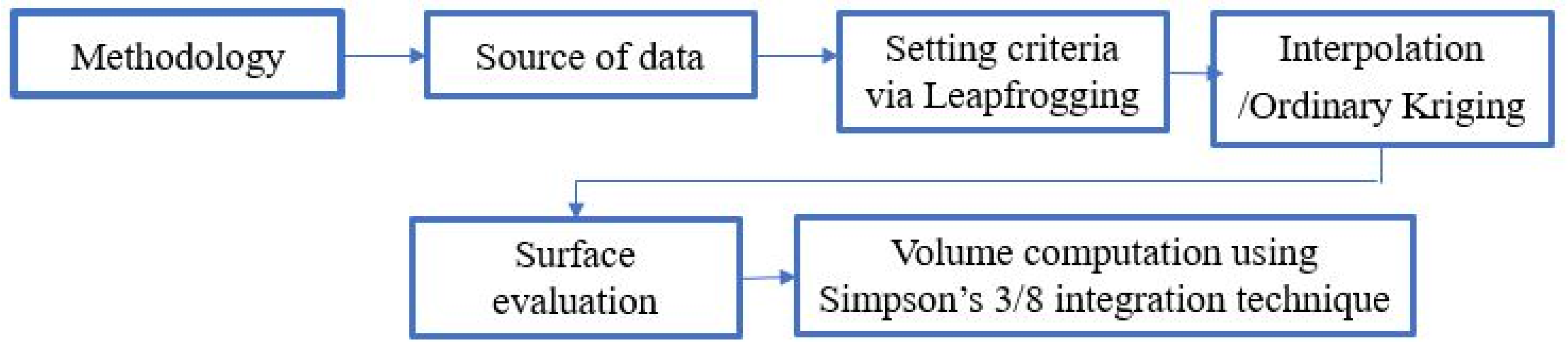
2. Material and Method

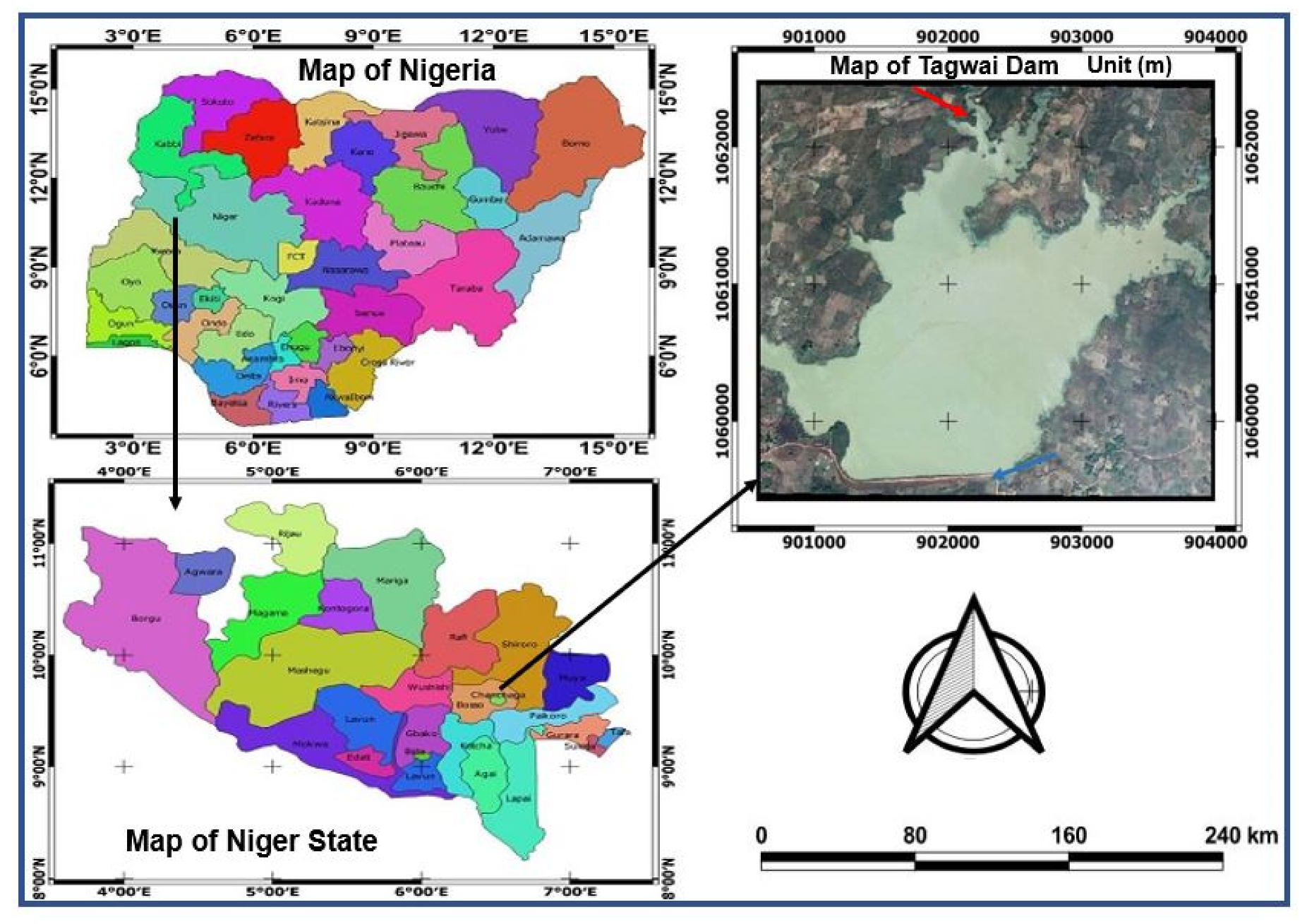
2.1. Study Area

The study area for this research work is Tagwai dam reservoir located in Bosso Local Government Area (LGA), in the south-west zone of Minna. The dam lies on latitude 90°34′9.23″ N and longitude 60°39′9.40″ E, 90°34′45.37″ N and 60°40′23.90″ E. The dam is located east of Tunga-goro, about 10 km south-east of Tunga-goro Market. The dam is an earth-fill dam and was constructed in the year 1978 by the Niger State Water Resources and Engineering Construction Agency. Figure 1 shows the location of the study area, the red arrow shows the Tagwai river, which is the major catchment area that supplies water to the dam throughout the seasons. Similarly, the blue arrow shows the dam axis and the only access road to the reservoir.

The principal occupations of the people settled within the dam environment are farming and fishing. The dam is under the care of the Niger State Water Board. Tagwai dam serves primarily as a reservoir for the supply of water to the city of Minna, the largest metropolis in Niger State.

The output of any research depends largely on the material and method used in conducting the investigation. Figure 2 describes the methodology adopted in this research.

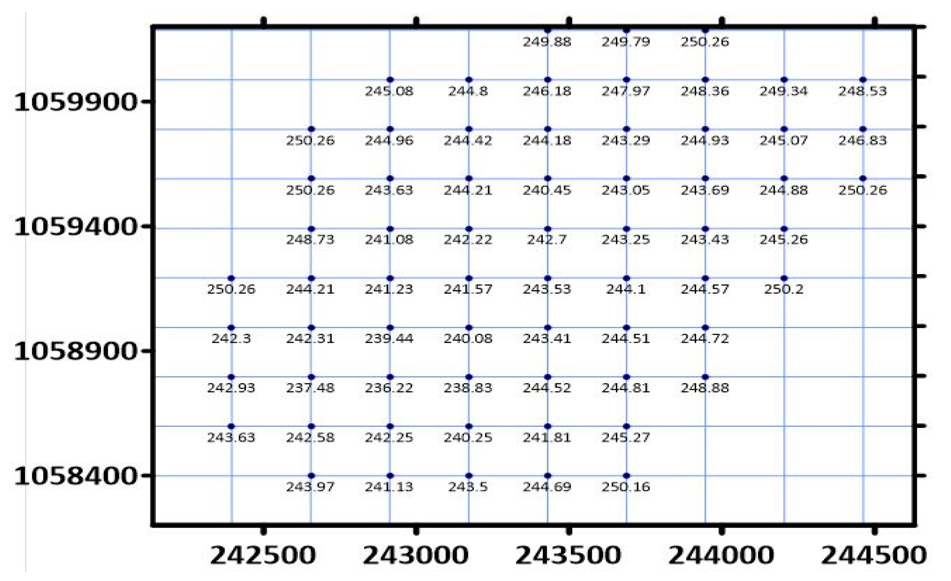
2.2. Source of Data

The sounding data were acquired using an EchoMap 50 s single-beam echosounder on a manned vessel at 25 m interval strips and a 50 m interval cross-section. Similarly, the sound velocity in freshwater was used during the sounding operation. A differential global positioning system (Hi-Target V30) was used to delineate the dam shoreline. Tagwai dam bathymetric data were explicitly collected for research purposes by the authors. The data were corrected for all uncertainty. Additionally, a detailed review of uncertainty reduction can be found in [21,22]. The data might have been used by the researchers in another study, but most assuredly for different purposes. The total area of the reservoir at the instant of the survey was 3,020,344.936 m² (302.035 hectares) with a perimeter of 8728.358 m. The maximum depth observed was 20.800 m. The reduced water level at the moment of sounding was 250.170 m, as referenced to a sounding datum established around the corridor of the reservoir. The maximum and minimum elevation was 250.260 m and 229.460 m, respectively. The datum used was the Minna-UTM zone 32 projection system. The Minna datum was established based on Clark 1880 ellipsoidal parameters.

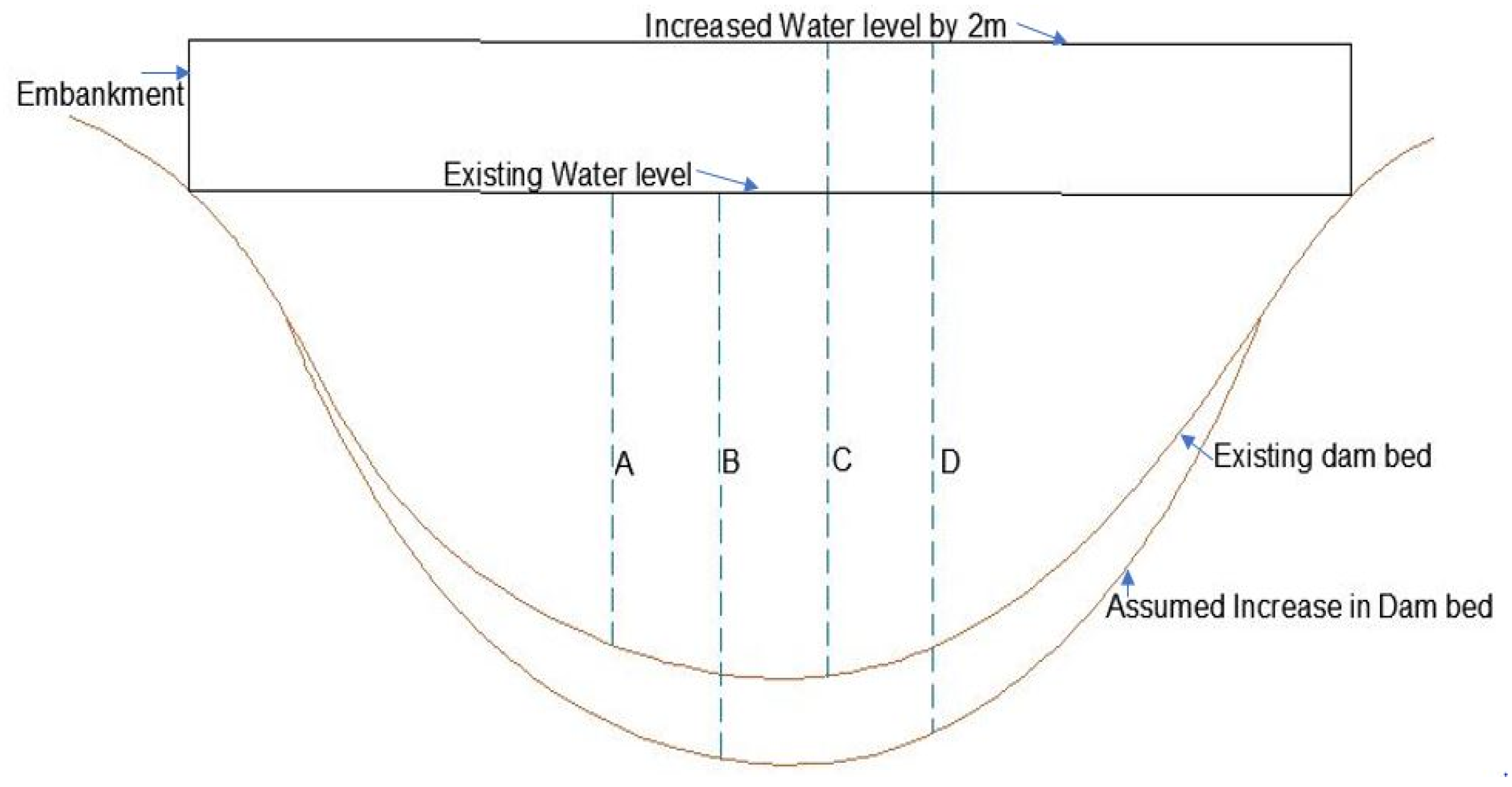
2.3. Setting Criteria and Scenario via Leapfrogging

Leapfrog, in this case, assumed that all the bathymetric points (points in blue) as shown in Figure 3, are the known leapfrog positions. Using the concept of leapfrogging as they leap upward or dig downward, there is a change in depth or height that affects the volume relative to space. Thus, four Scenarios were used to determine and enhance the capacity of the dam from leapfrog behavior. These scenarios are also called stages A, B, C, and D, respectively, as shown in Figure 4. The reason is to reduce ambiguity in writing.

The idea behind the leapfrogging applied, was that spatial information was treated independently, and they experienced change above the water level and below the reservoir base (waterbed) of 2 m, respectively. In each case, the data were interpolated using the ordinary Kriging interpolation technique.

2.4. Interpolation and Kriging

Interpolation is the act of using a discrete set of known data points to estimate for the unsampled area using mathematical and statistical functions within the original data set [12,23,24,25]. Overall interpolation is grouped into deterministic and geostatistics. Deterministic models utilize mathematical functions for estimation such as triangulation irregular networks, inverse distance weighting, etc., while probabilistic models, on the other hand, incorporate both the mathematical process and statistical models; “this allows spatial surfaces creation without interruption and predicting the parameter that measures the dispersion in the range of the measured values” [25], such as Kriging. There are different types of Kriging: Ordinary Kriging and universal Kriging. They are differentiated based on the drift factor. An experiment without a drift type is referred to as ordinary Kriging, while an experiment with a linear or quadratic drift type is known as universal Kriging. For more discussion on estimation models, see [25,26,27].

Furthermore, due to the use of a single-beam echosounder to acquire the bathymetric data, interpolation is necessary. This is required to account for the sparse area, and for DEM and volume determination. Therefore, before the data were interpolated, the bathymetry data were filtered to remove duplicated points. The shoreline data were extracted and added to the sounding data to delineate the dam and ensure that the estimated value does not cross the boundary. Consequently, the ordinary Kriging (OK) interpolation method was adopted to interpolate the data for this research. Kriging was employed because it assumes that the mean varies throughout the area of interest and that each local region has its mean. However, to certify some basic phenomena, a freefall hypothesis can be applied, which is the intrinsic hypothesis or semivariogram stationarity [25,26,28]. The semivariogram is mostly referred to as a variogram [29]. Additionally, this method was adopted in this study because it considers data anisotropy. Ordinary Kriging is expressed as:

$$Z\left(x\right)={{\displaystyle \sum }}_{i=1}^n{W}_i{Z}_i$$

(1)

where $Z\left(x\right)$ is the predicted value at any given unknown point, and $Z_i$ is the known or observed value at a point i. $W_i$ is the weight value assigned at point i. In particular, the weight coefficient $W_i$ is assigned considering the distance and spatial relationship between the known and unknown points. Consequently, to avoid biased results, the following condition must be satisfied.

$${{\displaystyle \sum }}_{i=1}^n{W}_i=1$$

(2)

while the error variance is given as:

$${\delta }^2=\frac{{{\displaystyle \sum }}_{i=1}^n{\left(Z_x-Z_i\right)}^2}{n}$$

(3)

where n is the total number of data points. However, to reduce the degree of error variance, the derivatives of Equation (3) over each weight should equal zero, and is expressed as a $\left(n+1\right)$ matrix model alongside the Lagrange parameter (µ) [27];

$$\left[\begin{array}{ccccc}0& {\gamma }_{1,2}& \dots & {\gamma }_{1,2}& 1\\ {\gamma }_{2,1}& 0& \dots & {\gamma }_{2,n}& 1\\ ⋮& ⋮& ⋮& ⋮& 1\\ {\gamma }_{n,1}& {\gamma }_{n,2}& \dots & 0& 1\\ 1& 1& \dots & 1& 0\end{array}\right].\left[\begin{array}{c}{w}_1\\ w_2\\ ⋮\\ w_n\\ -\mu \end{array}\right]=\left[\begin{array}{c}{\gamma }_{1,x}\\ {\gamma }_{2,x}\\ ⋮\\ {\gamma }_{n,x}\\ 1\end{array}\right]$$

(4)

where $\gamma$ represents the semivariogram values from pairs of point 1 to n, and x is the point where the unknown value is estimated from the unknown (1 … n). The most crucial aspect of Kriging’s pliability is the variogram or semivariogram, and is mathematically expressed as:

$${\gamma }_{\left(h\right)}=\frac{1}{2N\left(h\right)}{{\displaystyle \sum }}_{i=1}^{N\left(h\right)}{\left[Z\left(x_i\right)-Z\left(x_i+h\right)\right]}^2$$

(5)

where ${\gamma }_{\left(h\right)}$ is the number of sample pairs with a distance $h$; $Z\left(x_i\right)$ and $Z\left(x_i+h\right)$ are sample values, and they are dependent on the lag distance $h$ at the pairs of data points. Manually obtaining a variogram by spinning the direction to the desired experimental output is referred to as OK anisotropy [30,31]. Hence, in this study, the ordinary Kriging weights were computed by studying the omnidirectional semivariogram in the presence of anisotropy.

2.5. Ordinary Kriging Interpolation Experiment

The ordinary Kriging method was conducted based on the point data technique. The following factors were used; the major and semi-minor axis length used was 1450 m in both directions, the maximum number of data to use was 24, and the minimum number of data to use was 6. These were done to prevent excessive exaggeration in the estimation. To further measure the data fluctuations, the experimental semivariogram was generated, as shown in Figure 5a,b. Additionally,

Table 1. Experimental variogram outputs (units in meters and percentages).

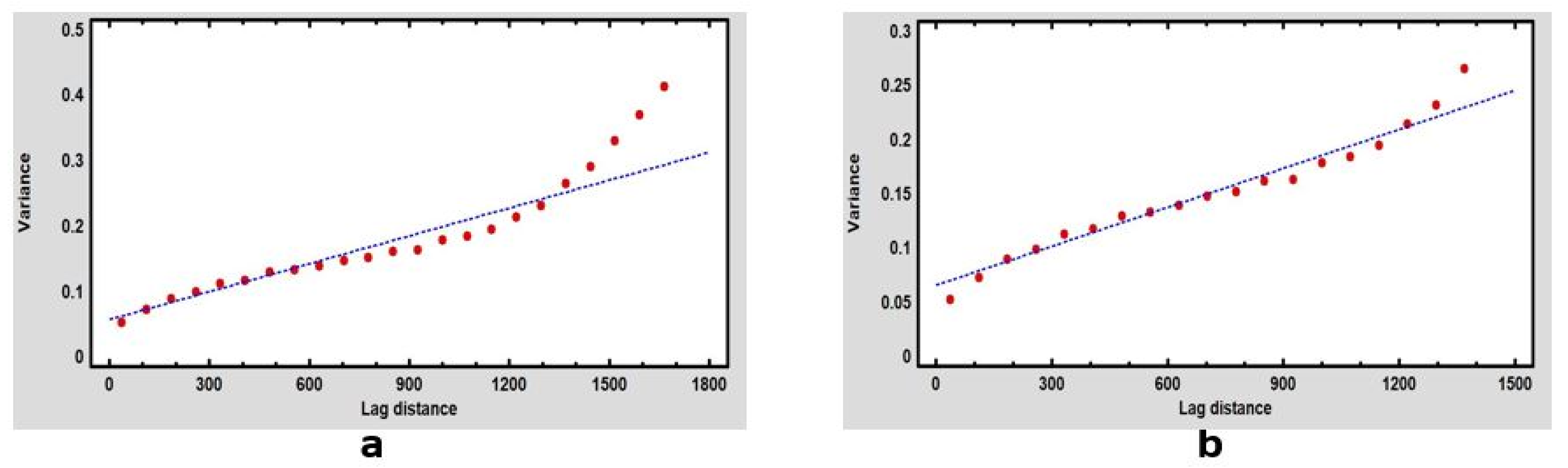
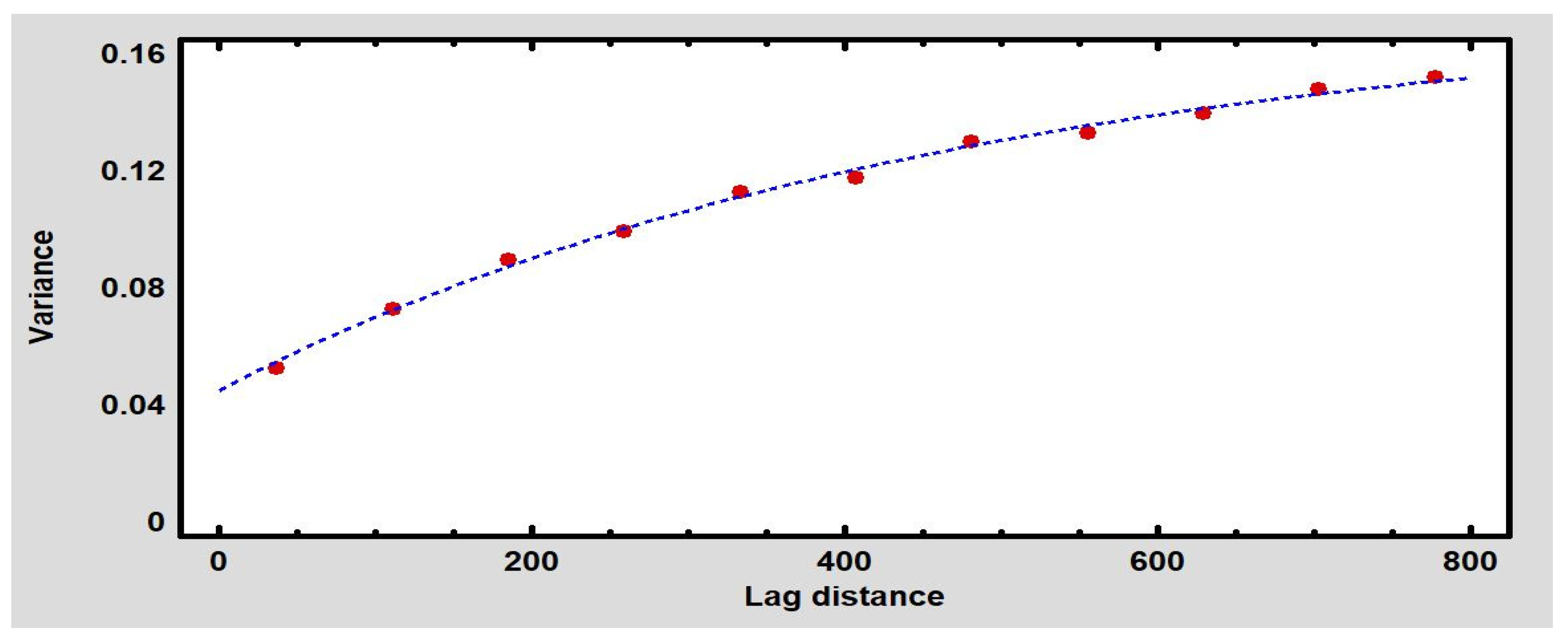
	Model	Nugget	Sill	Range	R-Squared	RMSE
Figure 5a	Exponential	0.075	0.421	1702.12	91.01%	0.165
Figure 5b	-	0.062	0.253	1425.20	92.63%	0.065
Figure 6	-	0.0451	0.157	775.21	99.58%	0.006

below shows the output parameters used for developing the initial and final experimental variogram.

Similarly, the final variogram was developed at 99.58% goodness of fit, with a root mean square error (RMSE) of 0.006, as shown in Table 1. Figure 6 shows the final experimental variogram developed. Generally, Figure 5a,b and Figure 6 show that, as the distance between two location increases, the variance increases, and as it reduces, the variance decreases.

These processes were conducted for all the scenarios considered and weighting was done repeatedly using $\raisebox{1ex}{$N_j$}\!\left/ \!\raisebox{-1ex}{$h^2{}_j$}\right.$, where $N_j$ is the number of pairs at a particular lag, and $h_j$ is the distance. However, for all the stages, the variogram is stationary; that is, all the variograms are highly similar (constant) [26]. Finally, grid $Z$ limits were set based on the data domain of 229.46 and 250.260 m, the first being the lowest $Z$ value, with the latter being the highest $Z$ value corresponding with the boundaries. Additionally, there is a spacing distance (resolution) of 15.125 m in both the X and Y directions to prevent excessive distance exaggeration based on the data trend.

2.6. Evaluation of Interpolation Surface

The cross-validation technique was conducted for the four stages to determine the data trend. Four hundred points were selected at random from the measured data for validation, as shown in Figure 7 and the outcome in

Table 2. Cross-validation results and volume output.

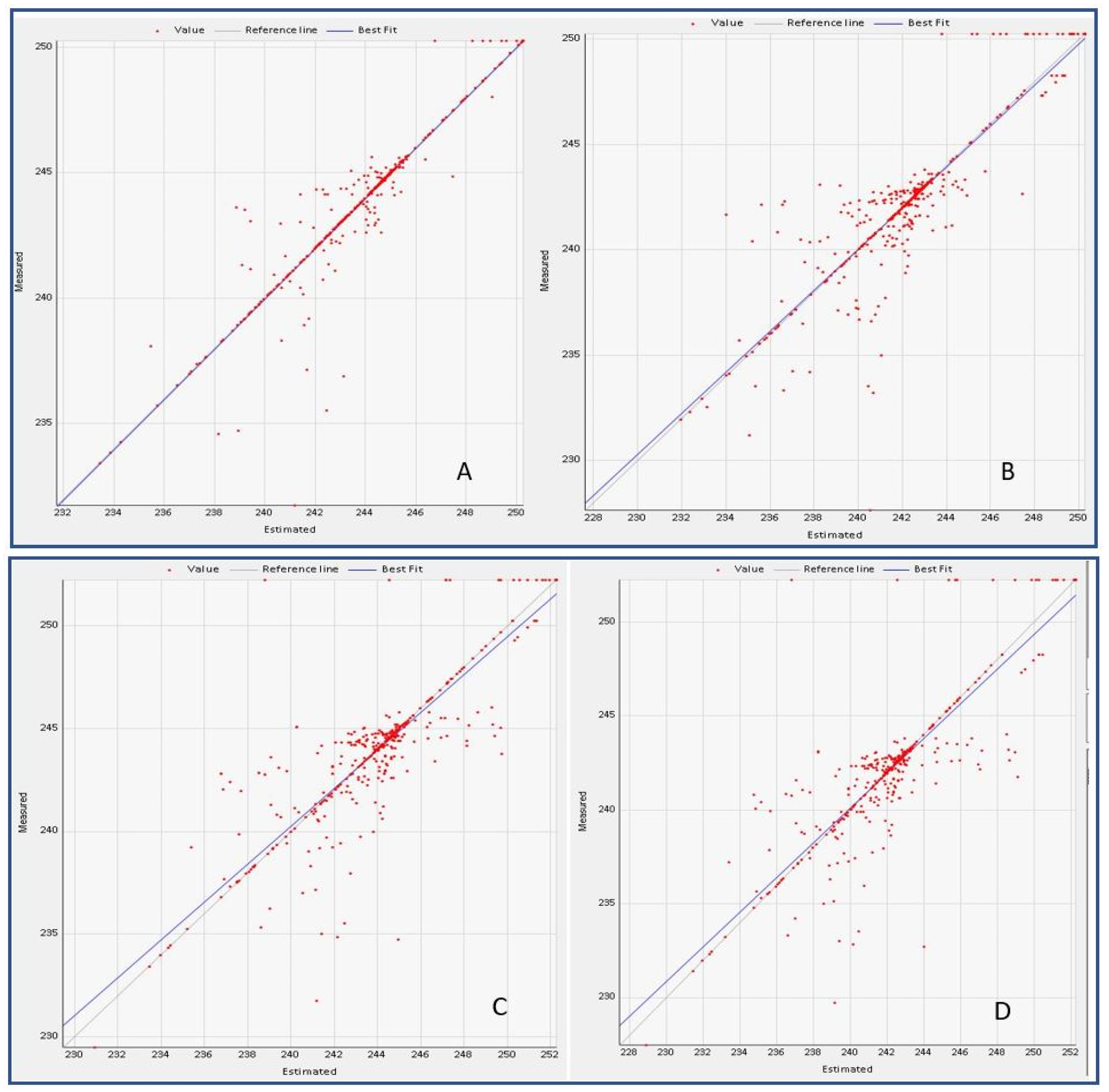
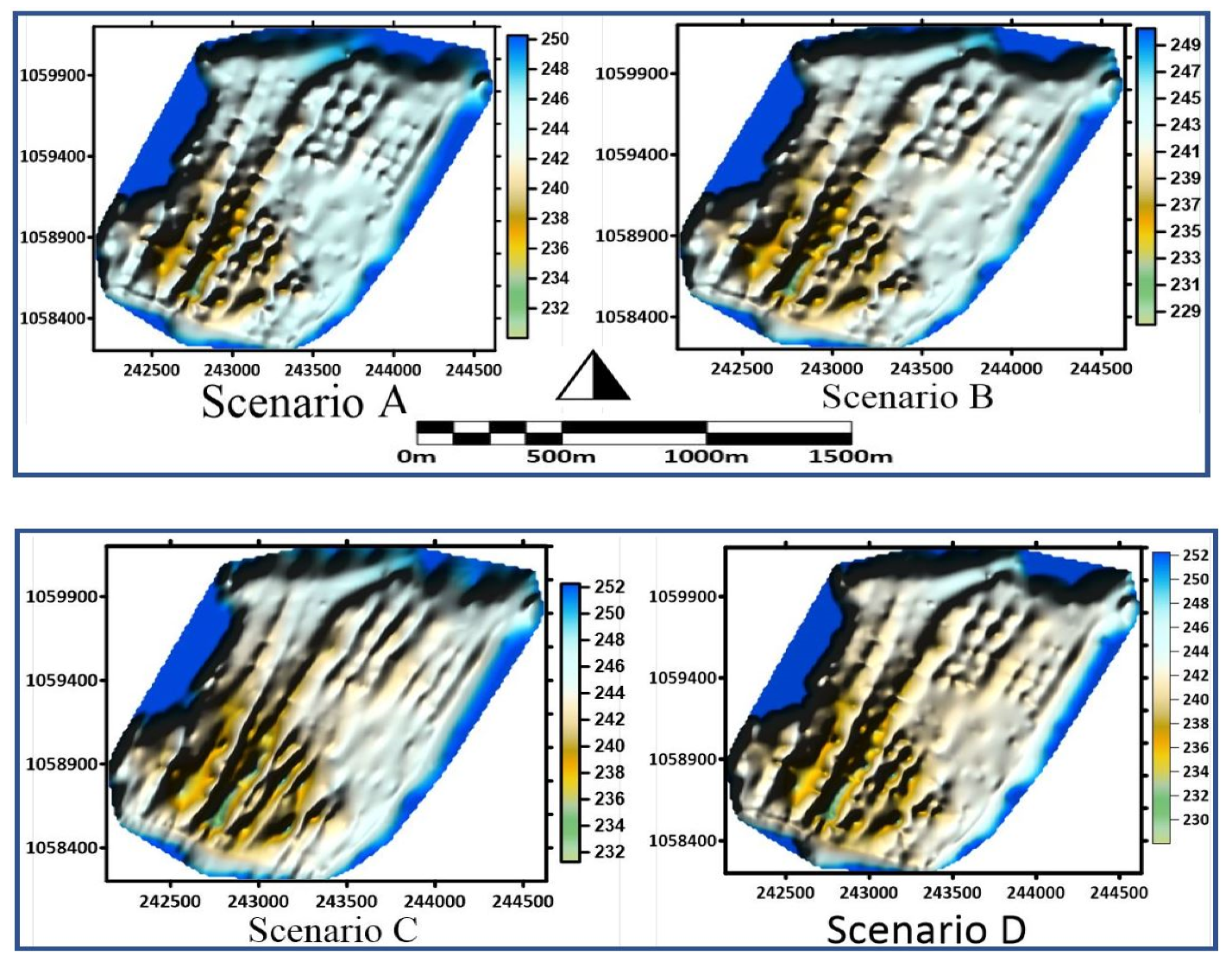
Scenario	ME	MSE	RMSE	R2	Coef. of Va.	Volume (m3)	% Volume
A	0.008	0.138	0.371	0.965	0.015	93,129,808	23.79
B	0.008	0.148	0.385	0.962	0.017	97,668,974	24.95
C	0.008	0.148	0.385	0.951	0.014	98,030,602	25.04
D	0.008	0.168	0.410	0.959	0.018	102,631,952	26.22

. Additionally, longitudinal and cross-sectional observations were carried out. Lines that ran perpendicular to the principal surveyed strips were checked to confirm the positioning’s accuracy. It was confirmed that the positional discrepancies were within the acceptable degree of freedom, according to [32]. Another validation medium applied is the withheld sample method; in this case, some observed samples were deliberately omitted before interpolation. After estimation, these points were tracked and their spatial attributes compared, as shown in

Table 3. Interactive cross-validation.

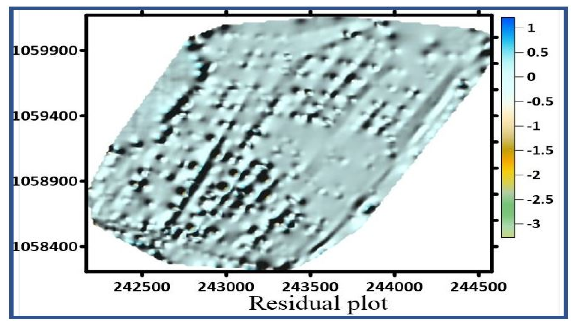
Easting (m)	Northing (m)	Reduced Depth (m)	Residuals (m)
242,502.387	1,058,741.722	242.414	0.006
243,107.042	1,058,271.965	244.086	−0.130
244,246.156	1,059,864.163	244.877	−0.004
242,885.429	1,059,116.951	236.219	0.207
243,209.73	1,059,435.427	242.708	−0.012

.

Furthermore, some selected quantitative methods of precision testing were employed, such as; the mean square error (MSE), the root mean square error (RMSE), the coefficient of multiple determination ($R^2)$, and the coefficient of variation in $Z$ axis. RMSE is used to determine the rate of error size; in contrast, it is sensitive to outliers due to the magnitude of weight it allocates to large errors [33]. Mean Error (ME) determine the level of bias in the output [34]; however, negative and positive predicted data should be taken into account [35]. The mathematical representation is given by [36,37,38,39] as:

$$MSE=\frac{1}{n}{{\displaystyle \sum }}_{i=1}^n{\left({\widehat{Z}}_i-Z_i\right)}^2$$

(6)

while the root mean square error is given as:

$$RMSE=\sqrt{\frac{{{\displaystyle \sum }}_{i=1}^n{\left({\widehat{Z}}_i-Z_i\right)}^2}{n}}$$

(7)

where $Z_i=$ the observed value, ${\widehat{Z}}_i=$ the predicted value and $n=$ the total number of points considered in Equations (6) and (7), respectively. Additionally, the mean error is computed as:

$$ME=\frac{{{\displaystyle \sum }}_{i=1}^n(Z_i^{PRED}-Z_i^{OBS})}{n}$$

(8)

where $Z_i^{PRED}$ and $Z_i^{OBS}$ are the predicted and observed depths, and n is the total number of observations. The statistical models are used to test the performance of the experiment; when they tend to zero, it shows the reliability of the interpolation technique.

2.7. Volume Computation via Simpson 3/8 Integration Techniques

Furthermore, Simpson’s 3/8 rule was used to compute the volume in each scenario considered. This volume computation method utilizes cubic interpolation instead of quadratic interpolation, as demonstrated in Equations (9) and (10) below.

$$\begin{array}{ll}Volume\left(m^3\right)& =\frac{3h}{8}\{f\left(X_0\right)+3f\left(X_1\right)+3f\left(X_2\right)+f\left(X_3\right)+f\left(X_3\right)\\ & +3f\left(X_4\right)+3f\left(X_5\right)+f\left(X_6\right)+\dots +f\left(X_{n-3}\right)\\ & +3f\left(X_{n-2}\right)+3f\left(X_{n-1}\right)+f\left(X_n\right)\}\end{array}$$

(9)

In particular, Equation (9) is integrated and presented as;

$$\begin{array}{ccc}Volume\left(m^3\right)& =& \frac{3h}{8}\{f\left(X_0\right)+3{{\displaystyle \sum }}_{i=1,4,7}^{n-2}f\left(X_i\right)+3{{\displaystyle \sum }}_{i=2,5,8}^{n-1}f\left(X_i\right)\\ & +& 3{{\displaystyle \sum }}_{i=3,6,9}^{n-3}f\left(X_n\right)\}\end{array}$$

(10)

where $n$ is the number of segments; $h$ is the vertical distance or elevation and, in this case, the reduced depth, and $X$ is the area.

3. Results and Analysis

Table 2 shows the output results from cross-validation analysis and volume computation of all the Scenarios considered. From Table 2, it is observable that the ME is in agreement in all the leapfrog stages and that there is no bias in the adopted method of interpolation and experimental performance. However, the MSEs of Scenarios B and C are correlated, but A and D show a small difference. The outcome of the MSE has a significant impact on the RMSE, as seen in Table 2. Consequently, the results for the RMSE reflect the weight of the MSE, because it is sensitive to outliers and influences large errors; hence, the MSE and RMSE suffer the same setback [32]. The experiment revealed that there is no unique correlation in the R² or coefficient of determination, but partial agreement in the coefficient of variance in all cases. The cross-validation result indicates a spatial trend of homogeneity in the estimation model in all classes. Furthermore, Table 3 shows the interactive cross-validation experiment in each case, five points were omitted from the original data and after interpolation, the points were tracked and their difference computed.

The interactive performance check shows that the points with a negative sign are above the measured surface, while the ones with a positive value are below the original data. The small change in the residual indicates that the estimated surface is dependable. In contrast, if the data are not properly distributed, there will be force exaggeration in predicted data which will then present a false surface. This confirmed that interpolation for the extraction of depth information should not be relied on entirely for critical engineering projects, but for reference purposes.

The omitted method of performance measurement is also called the direct method of accuracy investigation. If the results from this technique tend to zero then the output surface is positively correlated with the original surface. In addition, the spatial difference between the estimated value and the observed value was computed. Figure 8 shows the spread of residuals. The residuals show that the difference between the interpolated data and the observed data lies in the range of 1–3.

Figure 9 is the digital elevation model (DEM) of Scenarios A, B, C, and D; it describes the reservoir bed configuration. The present cubic content of leapfrog at rest (A) was calculated to be 93,129,808 m³, which is 23.79% of the total volume, as shown in Table 2. Subsequently, in Table 2 are the enhanced volume of other stages. Scenarios B and C account for 1.16% and 1.25% increases in volume above the present stage (A). Either B or C can be achieved by dredging or erecting an embankment around the dam of 2 m at any instant. Similarly, D is the combination of Scenario B and C, while A remains constant. Stage D has the edge over B and C of 2.43%, which is a 9,502,144 m³ increment above the present stage when implemented.

The waterbed trends of DEM B and D are symmetrical in nature, and this is supported by the coefficient of multiple determination ($R^2$) in Table 3. Thus, the DEM of A and C tend to follow suit, with a smooth outlines’ uniformity indicating a change in spatial data characteristics. Additionally, the area around the dam axis (southern part of each of Figure 9) is the deepest section of the basin. Thus, this section experiences sediment inflows from particles eroded uphill, especially during the precipitation period. In addition, the natural terrain model of the region exacerbates the rates of soil erosion within the catchment area, thereby aggravating the momentum of sediment deposits and, hence, decreases the depth and storage capacity.

4. Conclusions

The importance of dams for hydroelectricity, irrigation, and domestic uses has aided the development of humanity. However, reservoirs are challenged with the menace of sedimentation and siltation. The negative effect of concentrated particles in dams affects their functionality. The first stage of addressing this problem of sedimentation is conducting a bathymetric survey and producing a nautical chart or DEM that will better reveal the challenges for adequate planning. In this research, bathymetry and a shoreline delineation survey were conducted over Tagwai Dam. The data were interpolated using the ordinary Kriging method, and thereafter the leapfrogging approach was used to determine the present and enhanced volume at different Scenarios (A, B, C, and D). Scenarios B and C are achievable, but cost implicative. One challenge that may be encountered while carrying out stage B is getting in contact with rocks, but due to sediment deposits, this may not be a severe problem. One advantage of executing B is that the material can be used to erect Stage D, “a win-win situation”.

Furthermore, the results show that the volume increases at each leapfrogging method while the area remains constant relative to depth, following the existing pattern and shape of the reservoir. However, implementing both considerations to enhance the reservoir’s capacity shows that adequate volume can be added to the dam’s present state. Relief maps of all the postulated approaches were produced, depicting the terrain and waterbed configuration. There was no significant change in the area portrayed on the DEM because the shoreline remains constant. The results from the research will stand as a guide to the government and managers of the reservoir. The study suggested that Scenarios B and C should be considered to enhance the basin’s trapping capacity and reduce cost.

References

- David, D.; Hart, N.; Leroy, P. A Special Section on Dam Removal and River Restoration. BioScience 2002, 52, 653–655. [Google Scholar] [CrossRef]
- Ajith, A.V. Bathymetric Survey to Study the Sediment Deposit in Reservoir of Peechi Dam. IOSR J. Mech. Civ. Eng. 2016, 12, 34–38. [Google Scholar] [CrossRef]
- Amano, K. Water Quality Enhancement Techniques in Dam Reservoirs. J. Soc. Mech. Eng. 2003, 106, 454–455. [Google Scholar] [CrossRef]
- Girish, G.; Ashitha, M.K.; Jayakumar, K.V. Sedimentation assessment in a multipurpose reservoir in Central Kerala, India. Environ. Earth Sci. 2014, 72, 4441–4449. [Google Scholar] [CrossRef]
- Estigoni, M.; Matos, A.; Mauad, F. Assessment of the accuracy of different standard methods for determining reservoir capacity and sedimentation. J. Soils Sediments 2014, 14, 1224–1234. [Google Scholar] [CrossRef]
- Hart, D.D.; Johnson, T.E.; Bushaw-Newton, K.L.; Horwitz, R.J.; Bednarek, A.T.; Charles, D.F.; Kreeger, D.A.; Velinsky, D.J. Dam Removal: Challenges and Opportunities for Ecological Research and River Restoration. BioScience 2002, 52, 669–682. [Google Scholar] [CrossRef]
- Badejo, O.T.; Adewuyi, K.G. Bathymetric Survey and Topography Changes Investigation of Part of Badagry Creek and Yewa River, Lagos State, Southwest Nigeria. J. Geogr. Environ. Earth Sci. Int. 2019, 22, 1–16. [Google Scholar] [CrossRef]
- Khattab, M.F.; Abo, R.K.; Al-Muqdadi, S.W.; Merkel, B.J. Generate Reservoir Depths Mapping by Using Digital Elevation Model: A Case Study of Mosul Dam Lake, Northern Iraq. Adv. Remote Sens. 2017, 6, 161–174. [Google Scholar] [CrossRef]
- Morris, L.M.; Fan, J. Reservoir Sedimentation Handbook: Design and Management of Dams, Reservoirs, and Watersheds for Sustainable Use; McGraw-Hill: New York, NY, USA, 1998; p. 4.17. [Google Scholar]
- Lampe, D.C.; Morlock, S.E. Collection of bathymetric data along two reaches of the Lost River within Bluespring Cavern near Bedford, Lawrence County, Indiana. Sci. Investig. Rep. 2007, 142, 2008–5023. Available online: http://pubs.water.usgs.gov/sir (accessed on 15 August 2020).
- Silveira, D.T.; Portugal, J.L.; de Oliveira Vital, S.R. Análise estatística espacial aplicada a construção de superfícies batimétricas. Geociências 2014, 33, 596–615. [Google Scholar]
- Farrira, I.O.; Dalto, D.R.; Gérson, R.S.; Lidiane, M.F. In Bathymetric Surfaces: IDW Or Kriging. Bol. Ciênc. Geod. 2017, 23, 493–508. [Google Scholar] [CrossRef]
- McIntire, J.P.; Webber, F.C.; Nguyen, D.K.; Li, Y.; Foong, S.H.; Schafer, K.; Chue, W.Y.; Ang, K.; Vinande, E.T. LeapFrogging: A technique for accurate long-distance ground navigation and positioning without GPS. J. Inst. Navig. 2018, 65, 35–47. [Google Scholar] [CrossRef]
- Fudenberg, D.; Gilbert, R.; Stiglitz, J.; Tirole, J. Preemption, Leapfrogging, and Competition in Patent Races. Eur. Econ. Rev. 1983, 22, 3–31. [Google Scholar] [CrossRef]
- Brezis, E.; Krugman, P.; Tsiddon, D. Leapfrogging: A Theory of Cycles in National Technological Leadership. Am. Econ. Rev. 1993, 1211–1219. [Google Scholar] [CrossRef]
- Brezis, E.S.; Krugman, P. Technology and Life Cycle of Cities. J. Econ. Growth 1997, 2, 369–383. [Google Scholar] [CrossRef]
- Munasinghe, M. Is environmental degradation an inevitable consequence of economic growth: Tunneling through the environmental Kuznets curve. Ecol. Econ. 1999, 29, 89–109. [Google Scholar] [CrossRef]
- Barro, R.; Sala-i-Martin, X. Economic Growth; MIT Press: Cambridge, MA, USA, 2003; p. 375. ISBN 9780262025539. [Google Scholar]
- Arseni, M.; Voiculescu, M.; Georgescu, L.P.; Iticescu, C.; Rosu, A. Testing Different Interpolation Methods Based on Single Beam Echosounder River Surveying. Case Study: Siret River. Int. J. Geo-Inf. 2019, 8, 507. [Google Scholar] [CrossRef]
- Parente, C.; Vallario, A. Interpolation of Single Beam Echo Sounder Data for 3D Bathymetric Model. Int. J. Adv. Comput. Sci. Appl. 2019, 10, 6–13. [Google Scholar] [CrossRef]
- IHO Manual on Hydrography. International Hydrographic Organization Publication C-13; International Hydrographic Bureal: Monaco City, Monaco, 2011. [Google Scholar]
- Hare, R.; Eakins, B.; Amante, C. Modelling Bathymetric Uncertainty. Int. Hydrogr. Rev. 2011, 6, 31–42. Available online: https://coast.noaa.gov/data/digitalcoast/pdf/topo-bathy-data-considerations.pdf (accessed on 15 August 2020).
- Williams, C.K.I. Prediction with Gaussian Processes: From Linear Regression to Linear Prediction and Beyond. Learn. Graph. Models 1998, 599–621. [Google Scholar] [CrossRef]
- Marcelo, C.; Joaquim, L.; Igor, O.; Joao, L.; Jose, S. Assessment of Spatial Interpolation Methods to Map Bathymetry of an Amazonian Hydroelectric reservoir to Aid in decision marking for water Management. ISPRS Int. J. Geo-Inform. 2015, 4, 220–235. [Google Scholar] [CrossRef]
- Ferreira, I.O.; Domingos, R.D.; Santos, G.R. Coleta, Processamento e Análise de Dados Batimétricos; Novas Edições Acadêmicas: do Paraná, Brazil, 2015. [Google Scholar]
- Li, J.; Heap, A.D. Spatial interpolation methods applied in the environmental sciences: A review. Environ. Model Softw. 2014, 53, 173–189. [Google Scholar] [CrossRef]
- Wu, C.; Joann, M.; Liang, M.; Mohammad, A. Comparison of different spatial interpolation methods for historical hydrographic data of the lowermost Mississippi River. Ann. GIS 2019, 25, 133–151. [Google Scholar] [CrossRef]
- Santos, G.R.; Oliveira, M.S.; Louzada, J.M.; Santos, A.M.R.T. Krigagem simples versus krigagem universal: Qual o preditor mais precison. Energy Agric. 2011, 26, 49–55. [Google Scholar] [CrossRef]
- Webster, R.; Oliver, M. Geostatistics for Environmental Scientists; John Wiley & Sons, Ltd.: Chichester, UK, 2001; p. 271. [Google Scholar]
- Eriksson, M.; Siska, P.P. Understanding Anisotropy Computations. Math. Geol. 2000, 32, 683–700. [Google Scholar] [CrossRef]
- Merwade, V.M.; Maidment, D.R.; Goff, J.A. Anisotropic considerations while interpolating river channel bathymetry. J. Hydrol. 2006, 331, 731–741. [Google Scholar] [CrossRef]
- Canadian Hydrographic Service (CHS). CHS Standards for Hydrographic Surveys, 1st ed.; Fisheries and Oceans: Ottawa, ON, Canada, 2005. [Google Scholar]
- Hernandez-Stefanoni, J.L.; Ponce-Hernandez, R. Mapping the spatial variability of plant diversity in a tropical forest: Comparison of spatial interpolation methods. Environ. Monit. Assess. 2006, 117, 307–334. [Google Scholar] [CrossRef]
- Isaaks, E.H.; Srivastava, R.M. Applied Geostatistics; Oxford University Press: New York, NY, USA, 1989; p. 561. [Google Scholar]
- Nalder, I.A.; Wein, R.W. Spatial interpolation of climatic Normals: Test of a new method in the Canadian boreal forest. Agric. For. Meteorol. 1998, 92, 211–225. [Google Scholar] [CrossRef]
- Ahmed, S.; De Marsily, G. Comparison of geostatistical methods for estimating transmissivity using data on transmissivity and specific capacity. Water Resour. Res. 1987, 23, 1717–1737. [Google Scholar] [CrossRef]
- Burrough, P.A.; McDonnell, R.A. Principles of Geographical Information Systems; Oxford University Press: Oxford, UK, 1998; p. 333. [Google Scholar]
- Hu, K.; Li, B.; Lu, Y.; Zhang, F. Comparison of various spatial interpolation methods for non-stationary regional soil mercury content. Environ. Sci. 2004, 25, 132–137. [Google Scholar]
- Vicente-Serrano, S.M.; Saz-Sánchez, M.A.; Cuadrat, J.M. Comparative analysis of interpolation methods in the middle Ebro Valley (Spain): Application to annual precipitation and temperature. Clim. Res. 2003, 24, 161–180. [Google Scholar] [CrossRef]