Monitoring and Mapping of Shallow Landslides in a Tropical Environment Using Persistent Scatterer Interferometry: A Case Study from the Western Ghats, India


 ,
,  ,
, 
Abstract
:1. Introduction
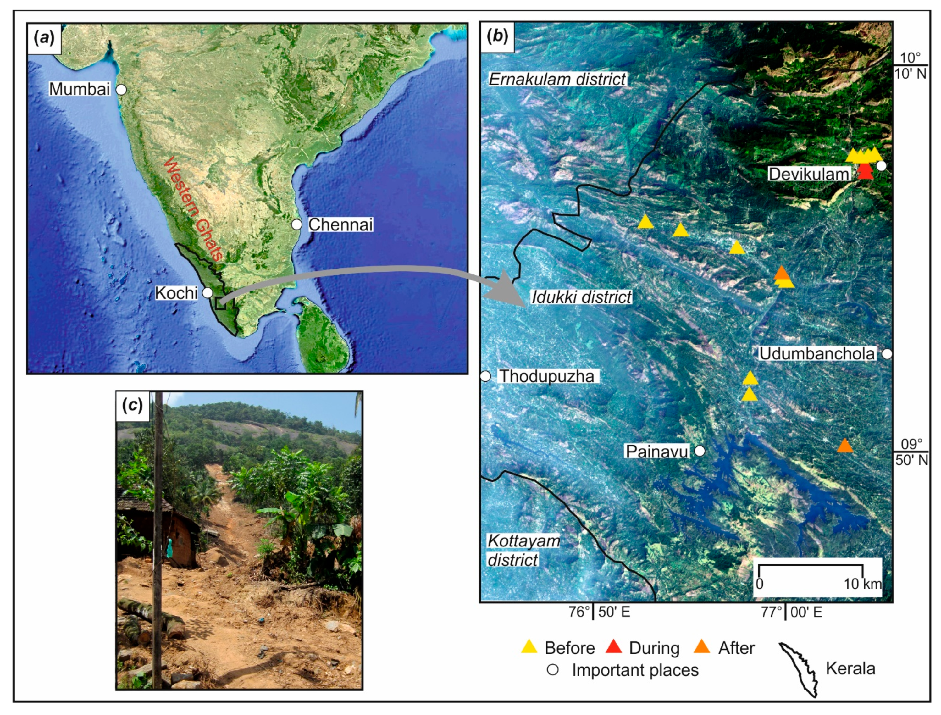
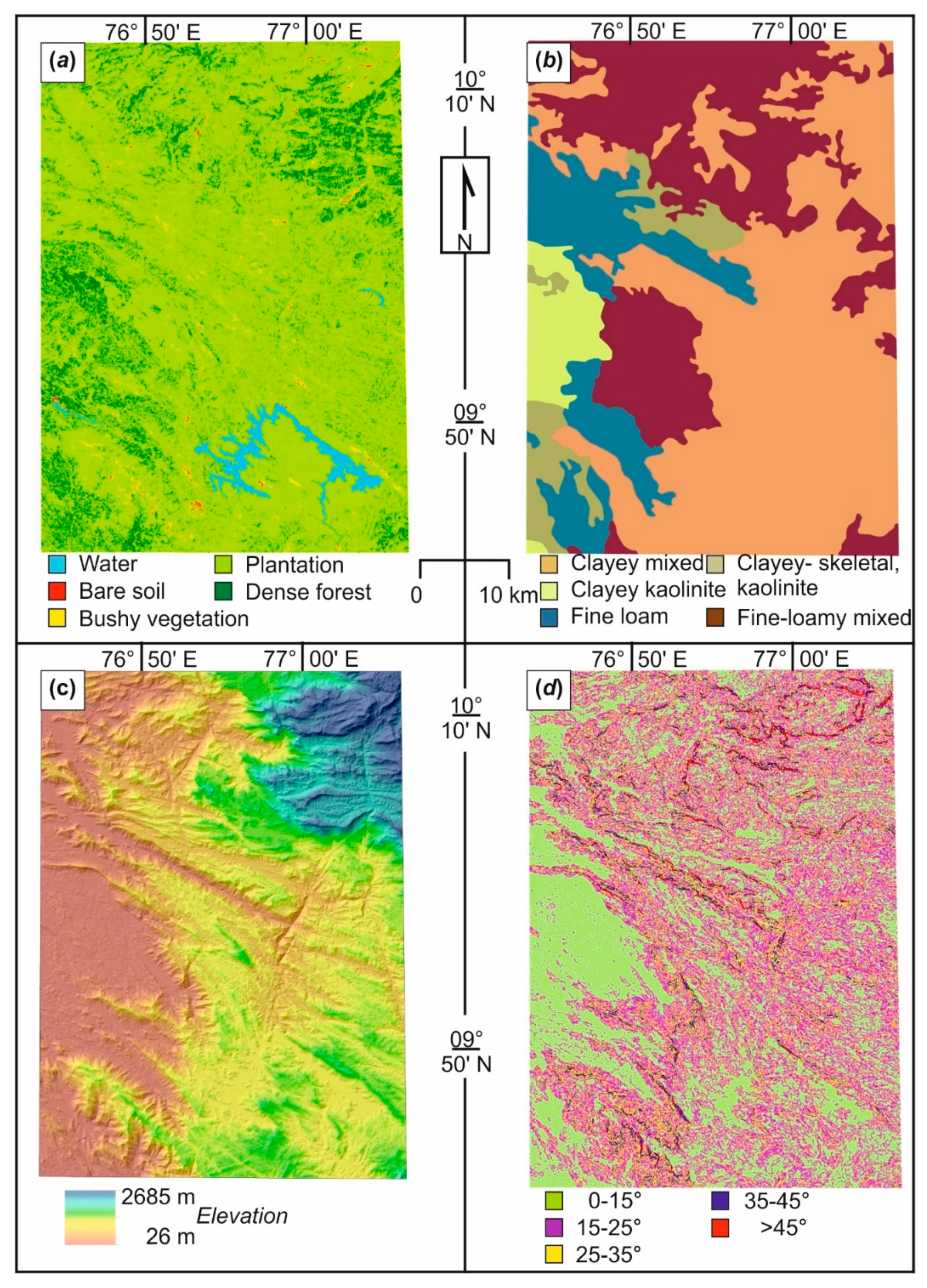
2. Study Area
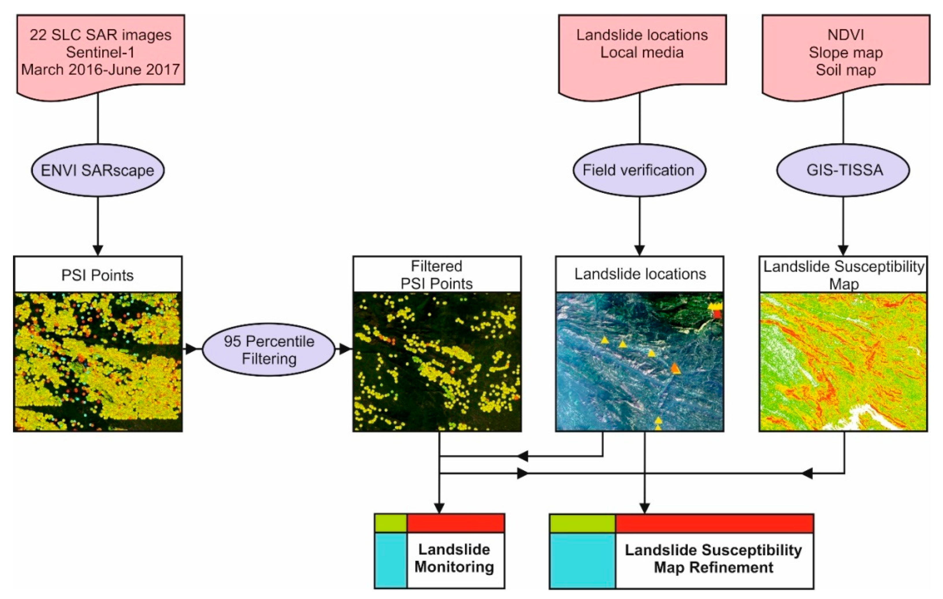
3. Data and Methodology
3.1. Selection of Landslide Location
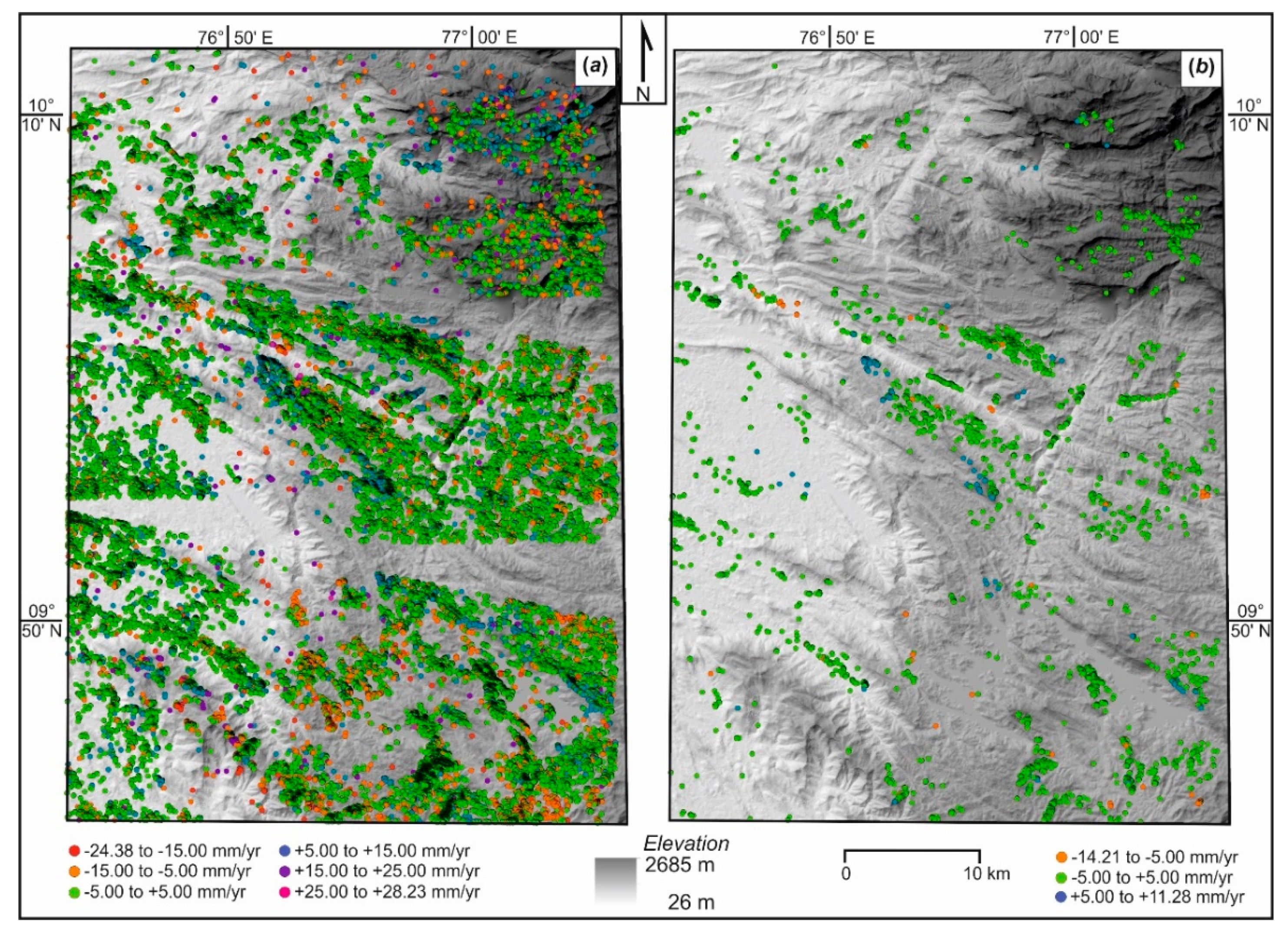
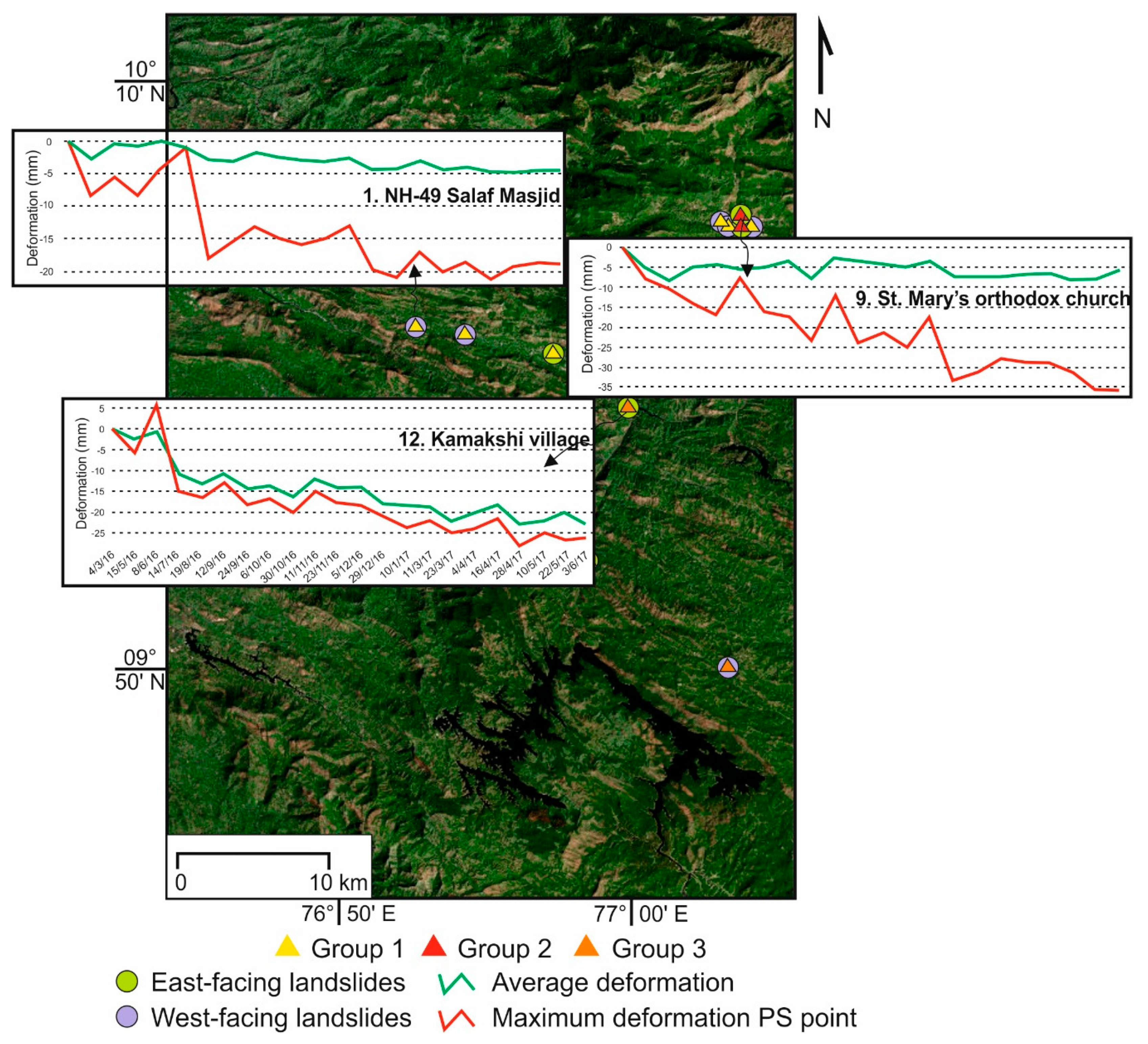
3.2. Monitoring of Individual Landslides
- Negative velocity values on west-facing slopes, indicating downward or westward (downslope) movement, and
- Positive velocity values on east-facing slopes, indicating downward or eastward (downslope) movement.
3.3. Filtering of PSI Points
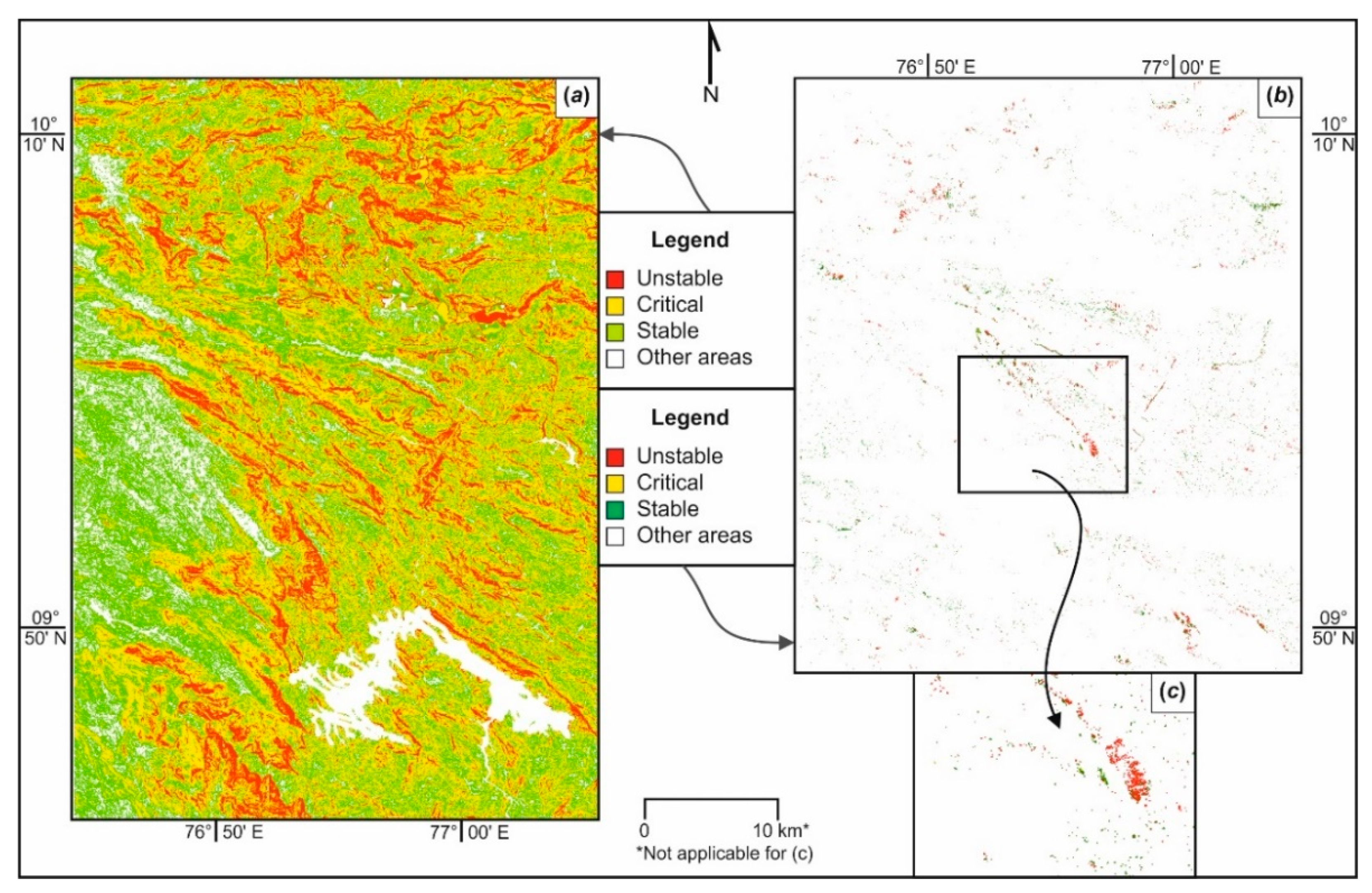
3.4. Creation of Slope Stability Map
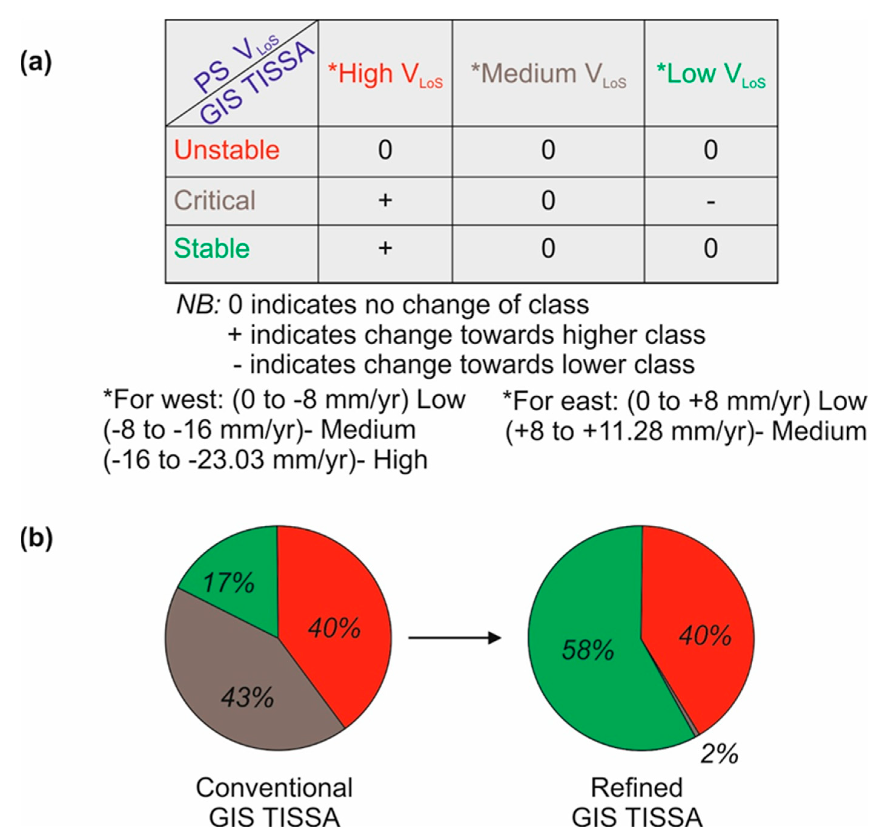
3.5. Refinement of Slope Stability Map
4. Results
4.1. Monitoring Shallow Debris Flows
4.2. Mapping and Refining the Conventional FS Map
5. Discussion
6. Conclusions
- The three types of temporal landslides pertaining to different periods of PSI analysis resulted in providing three distinct PSI velocity values. These refer to landslides that occurred before the analyzed time period, during PSI analysis, and after the analysis.
- Traditional slope stability analysis methods often lead to significant false positives. The proposed approach combining PSI with traditional slope stability shows promise in reducing these false positives. The PSI derived velocity was used to refine the existing landslide susceptibility map. Such refinement will help to identify areas that require utmost priority in terms of monitoring or mitigation.
- Developing countries like India will only have limited financial provisions for adopting management practices. The freely available radar data and the provisions of identifying areas requiring urgent management are able to be deciphered through studies like the one mentioned here.
- Such an approach could also help the engineering community gain better community confidence as the slope stability model is more targeted and less susceptible to false positives.
Supplementary Materials
Author Contributions
Funding
Institutional Review Board Statement
Informed Consent Statement
Data Availability Statement
Acknowledgments
Conflicts of Interest
References
- Piciullo, L.; Calvello, M.; Cepeda, J.M. Territorial early warning systems for rainfall-induced landslides. Earth Sci. Rev. 2018, 179, 228–247. [Google Scholar] [CrossRef]
- Wieczorek, G.F. Landslides: Investigation and mitigation. In Landslides: Investigation and Mitigation, Special Report 247, Transportation Research Board, National Research Council; Turner, A.K., Schuster, R.L., Eds.; National Academy Press: Washington, DC, USA, 1996; pp. 76–90. [Google Scholar]
- Zamenian, H.; Koo, D.D. Tunnel asset management (TAM) program application for high risk structural components. J. Eng. Archit. 2014, 2, 1–12. [Google Scholar] [CrossRef] [Green Version]
- Martinović, K.; Gavin, K.; Reale, C.; Mangan, C. Rainfall thresholds as a landslide indicator for engineered slopes on the Irish Rail network. Geomorphology 2018, 306, 40–50. [Google Scholar] [CrossRef] [Green Version]
- Naidu, S.; Sajinkumar, K.S.; Oommen, T.; Anuja, V.J.; Samuel, R.A.; Muraleedharan, C. Early warning system for shallow landslides using rainfall threshold and slope stability analysis. Geosci. Front. 2018, 9, 1871–1882. [Google Scholar] [CrossRef]
- Rossi, M.; Kirschbaum, D.; Valigi, D.; Mondini, A.C.; Guzzetti, F. Comparison of Satellite Rainfall Estimates and Rain Gauge Measurements in Italy, and Impact on Landslide Modeling. Climate 2017, 5, 90. [Google Scholar] [CrossRef] [Green Version]
- Smith, D.M.; Oommen, T.; Bowman, L.J.; Gierke, J.S.; Vitton, J. Hazard assessment of rainfall-induced landslides: A case study of San Vicente volcano in central El Salvador. Nat. Hazards 2015, 75, 2291–2310. [Google Scholar] [CrossRef]
- Cruden, D.M.; Varnes, D.L. Landslide types and processes. In Landslides: Investigation and Mitigation, Special Report 247, Transportation Research Board, National Research Council; Turner, A.K., Schuster, R.L., Eds.; National Academy Press: Washington, DC, USA, 1996; pp. 36–75. [Google Scholar]
- Keaton, J.R.; De Graff, J.V. Surface observation and geologic mapping. In Landslides: Investigation and Mitigation, Special Report 247, Transportation Research Board, National Research Council; Turner, A.K., Schuster, R.L., Eds.; National Academy Press: Washington, DC, USA, 1996; pp. 178–230. [Google Scholar]
- Varnes, D.J. Slope movement types and processes. In Landslides: Analysis and Control, Special Report 176, Transportation Research Board, National Research Council; Schuster, R.L., Krizek, R.J., Eds.; National Academy Press: Washington, DC, USA, 1978; pp. 11–33. [Google Scholar]
- Thampi, P.K.; Mathai, J.; Sankar, G.; Sidharthan, S. Debris flow in Western Ghats-A regional evaluation. In Final Proceedings Tenth Kerala Science Congress; Kerala State Council for Science, Technology and Environment: Kozhikode, India, 1998; pp. 73–75. [Google Scholar]
- Sajinkumar, K.S.; Anbazhagan, S.; Rani, V.R.; Muraleedharan, C. A paradigm quantitative approach for a regional risk assessment and management in a few landslide prone hamlets along the windward slope of Western Ghats, India. Int. J. Disast. Risk Reduct. 2014, 7, 142–153. [Google Scholar] [CrossRef]
- Blaschke, T.; Lang, S.; Lorup, E.; Strobl, J.; Zeil, P. Object-oriented image processing in an integrated GIS/remote sensing environment and perspectives for environmental applications. Environ. Inf. Plan. Politics Public 2000, 2, 555–570. [Google Scholar]
- He, K.S.; Rocchini, D.; Neteler, M.; Nagendra, H. Benefits of hyperspectral remote sensing for tracking plant invasions. Divers. Distrib. 2011, 17, 381–392. [Google Scholar] [CrossRef]
- Li, X.; Yeh, A.G.O. Analyzing spatial restructuring of land use patterns in a fast growing region using remote sensing and GIS. Landscape Urban Plan. 2004, 69, 335–354. [Google Scholar] [CrossRef]
- Metternicht, G.; Hurni, L.; Gogu, R. Remote sensing of landslides: An analysis of the potential contribution to geo-spatial systems for hazard assessment in mountainous environments. Remote Sens. Environ. 2005, 98, 284–303. [Google Scholar] [CrossRef]
- Escobar-Wolf, R.; Oommen, T.; Brooks, C.N.; Dobson, R.J.; Ahlborn, T.M. Unmanned aerial vehicle (UAV)-based assessment of concrete bridge deck delamination using thermal and visible camera sensors: A preliminary analysis. Res. Nondestruct. Eval. 2018, 29, 183–198. [Google Scholar] [CrossRef]
- Devanthéry, N.; Crosetto, M.; Monserrat, O.; Cuevas-González, M.; Crippa, B. An Approach to Persistent Scatterer Interferometry. Remote Sens. 2014, 6, 6662–6679. [Google Scholar] [CrossRef] [Green Version]
- Ferretti, A.; Prati, C.; Rocca, F. Nonlinear subsidence rate estimation using permanent scatterers in differential SAR interferometry. IEEE Trans. Geosci. Remote Sens. 2000, 38, 2202–2212. [Google Scholar] [CrossRef] [Green Version]
- Ferretti, A.; Prati, C.; Rocca, F. Permanent scatterers in SAR interferometry. IEEE Trans. Geosci. Remote Sens. 2001, 39, 8–20. [Google Scholar] [CrossRef]
- Bouali, E.H.; Oommen, T.; Escobar-Wolf, R. Mapping of slow landslides on the Palos Verdes Peninsula using the California landslide inventory and persistent scatterer interferometry. Landslides 2018, 15, 439–452. [Google Scholar] [CrossRef]
- Casagli, N.; Frodella, W.; Morelli, S.; Tofani, V.; Ciampalini, A.; Intrieri, E.; Raspini, F.; Rossi, G.; Tanteri, L.; Lu, P. Spaceborne, UAV and ground-based remote sensing techniques for landslide mapping, monitoring and early warning. Geoenviron. Disasters 2017, 4, 1–23. [Google Scholar] [CrossRef]
- Cascini, L.; Peduto, D.; Pisciotta, G.; Arena, L.; Ferlisi, S.; Fornaro, G. The combination of DInSAR and facility damage data for the updating of slow-moving landslide inventory maps at medium scale. Nat. Hazards Earth Syst. Sci. 2013, 13, 1527–1549. [Google Scholar] [CrossRef]
- Gullà, G.; Peduto, L.; Antronico, L.; Fornaro, G. Geometric and kinematic characterization of landslides affecting urban areas: The Lungro case study (Calabria, Southern Italy). Landslides 2017, 14, 171–188. [Google Scholar] [CrossRef]
- Lu, P.; Catani, F.; Tofani, V.; Casagli, N. Quantitative hazard and risk assessment for slow-moving landslides from persistent scatterer interferometry. Landslides 2014, 11, 685–696. [Google Scholar] [CrossRef]
- Novellino, A.; Cigna, F.; Sowter, A.; Ramondini, M.; Calcaterra, D. Exploitation of the intermittent SBAS (ISBAS) algorithm with COSMO-SkyMed data for landslide mapping in north-western Sicily, Italy. Geomorphology 2017, 280, 153–166. [Google Scholar] [CrossRef]
- Schaefer, L.N.; Lu, Z.; Oommen, T. Dramatic volcanic instability revealed by InSAR. Geology 2015, 43, 743–746. [Google Scholar] [CrossRef] [Green Version]
- Schaefer, L.N.; Wang, T.; Escobar-Wolf, R.; Oommen, T.; Lu, Z.; Kim, J.; Lundgren, P.R.; Waite, G.P. Three-dimensional displacements of a large volcano flank movement during the May 2010 eruptions at Pacaya Volcano, Guatemala. Geophys. Res. Lett. 2017, 44, 135–142. [Google Scholar] [CrossRef] [Green Version]
- Sajinkumar, K.S. Geoinformatics in landslide risk assessment and management in parts of Western Ghats, Central Kerala, South India. Ph.D. Thesis, IIT Bombay, Mumbai, India, 2005, unpublished. [Google Scholar]
- Sajinkumar, K.S.; Oommen, T. Landslide Atlas of Kerala; Geological Society of India: Bangalore, India, 2020; p. 49. [Google Scholar]
- GSI. Geology and Mineral Resources of Kerala; Geological Survey of India: Thiruvananthapuram, India, 2005; p. 93. [Google Scholar]
- Nandakumaran, P.; Balakrishnan, K. Comparison of hydrochemical characteristics of shallow and depp aquifers in a hard rock terrain in Kerala, India. In Proceedings of the International Conference & Exhibition on Integrated Water, Waste Water and Isotope Hydrology, Bangalore, India, 25–27 July 2013. [Google Scholar]
- ASF: Alaska Satellite Facility Vertex: ASF’s Data Portal V3.04-54. Available online: https://vertex.daac.asf.alaska.edu/ (accessed on 8 September 2019).
- Crosetto, M.; Monserrat, O.; Cuevas-González, M.; Devanthéry, N.; Crippa, B. Persistent scatterer interferometry: A review. ISPRS J. Photogramm. Remote Sens. 2016, 115, 78–89. [Google Scholar] [CrossRef] [Green Version]
- Hooper, A.; Zebker, H.; Segall, P.; Kampes, B. A new method for measuring deformation on volcanoes and other natural terrains using InSAR persistent scatterers. Geophys. Res. Lett. 2004, 31, L23611. [Google Scholar] [CrossRef]
- Notti, D.; Herrera, G.; Bianchini, S.; Meisina, C.; Carlos, J.; Zicca, F. A methodology for improving landslide PSI data analysis. Int. J. Remote Sens. 2014, 35, 2186–2214. [Google Scholar] [CrossRef]
- USGS United States Geological Survey Earth Explorer. Available online: https://earthexplorer.usgs.gov/ (accessed on 8 September 2019).
- Holben, B.N. Characteristics of maximum-value composite images from temporal AVHRR data. Int. J. Remote Sens. 1986, 7, 1417–1434. [Google Scholar] [CrossRef]
- NBSS: National Bureau of Soil Survey. Soil Map of Kerala; National Bureau of Soil Science and Land Use Planning: Nagpur, India, 1996. [Google Scholar]
- JPL: Jet Propulsion Laboratory. Shuttle Radar Topography Mission, California Institute of Technology and the National Aeronautics and Space Administration. Available online: https://www2.jpl.nasa.gov/srtm/ (accessed on 3 July 2014).
- BIS: Bureau of Indian Standard. Indian Standard-Preparation of Landslide Hazard Zonation Maps in Mountainous Terrains-Guidelines; IS 14496 (Part 2); BIS: New Delhi, India, 1998; p. 20.
- Escobar-Wolf, R.; Sanders, J.; Vishnu, C.L.; Oommen, T.; Sajinkumar, K.S.A. GIS Tool for Infinite Slope Stability Analysis (GIS-TISSA). Geosci. Front. 2020. [Google Scholar] [CrossRef]
- Haneberg, W.C. PISA-m Map-based Probabilistic Infinite Slope Analysis: Version 1.0.1 User Manual [Updated March 2007]; Haneberg Geoscience: Seattle, WA, USA, 2007; p. 20. [Google Scholar]
- Stramondo, S.; Moro, M.; Tolomei, C.; Cinti, F.R.; Doumaz, F. InSAR surface displacement field and fault modelling for the 2003 Bam earthquake (southeastern Iran). J. Geodyn. 2005, 40, 347–353. [Google Scholar] [CrossRef]
- Lambiel, C.; Delaloye, R.; Strozzi, T.; Lugon, R.; Raetzo, H. ERS InSAR for assessing rock glacier activity. In Proceedings of the Ninth International Conference on Permafrost, Fairbanks, Alaska, 29 June–3 July 2008; Volume 1, pp. 1019–1025. [Google Scholar]
- Hu, J.; Li, ZW.; Ding, X.L.; Zhu, J.J.; Zhang, L.; Sun, Q. 3D coseismic displacement of 2010 Darfield, New Zealand earthquake estimated from multi-aperture InSAR and D-InSAR measurements. J. Geod. 2012, 86, 1029–1041. [Google Scholar] [CrossRef]
- Ciampalini, A.; Raspini, F.; Lagomarsino, D.; Catani, F.; Casagli, N. Landslide susceptibility map refinement using PSInSAR data. Remote Sens. Environ. 2016, 184, 302–315. [Google Scholar] [CrossRef]
- Bianchini, S.; Cigna, F.; Righini, G.; Proietti, C.; Casagli, N. Landslide HotSpot Mapping by means of Persistent Scatterer Interferometry. Environ. Earth Sci. 2012, 67, 1155–1172. [Google Scholar] [CrossRef]
- Cigna, F.; Bianchini, S.; Casagli, N. How to assess landslide activity and intensity with Persistent Scatterer Interferometry (PSI): The PSI-based matrix approach. Landslides 2013, 10, 267–283. [Google Scholar] [CrossRef] [Green Version]
- Mateos, R.M.; Azañón, J.M.; Roldán, F.J.; Notti, D.; Pérez-Peña, V.; Galve, J.P.; Pérez-García, J.L.; Colomo, C.M.; Gómez-López, J.M.; Montserrat, O.; et al. The combined use of PSInSAR and UAV photogrammetry techniques for the analysis of the kinematics of a coastal landslide affecting an urban area (SE Spain). Landslides 2017, 14, 743–754. [Google Scholar] [CrossRef]
- Oommen, T.; Cobin, P.F.; Gierke, J.S.; Sajinkumar, K.S. Significance of variable selection and scaling issues for probabilistic modeling of rainfall-induced landslide susceptibility. Spat. Inf. Res. 2018, 26, 21–31. [Google Scholar] [CrossRef]


| Age | Formation | Lithology |
|---|---|---|
| Recent | Alluvium | Sand, clay, riverine alluvium etc. |
| Sub-recent | Laterite | Derived from crystalline and sedimentary rocks |
| Tertiary | Warkalli Quilon Vaikom Alappuzha | Sandstone, clays with lignite Limestone, marl and clay Sandstone with pebbles, clay and lignite Carbonaceous Clay and fine sand |
| Undated | Intrusives | Dolerite, Gabbro, Granites, Quartzo-feldspathic veins |
| Archaean | Wayanad Group Charnockites Khondalites | Granitic gneiss, Schists etc. Charnockites and associated rocks Khondalite suite of rocks and its associates |
| S.No | Date of Image Acquisition | S.No | Date of Image Acquisition |
|---|---|---|---|
| 1 | 4 March 2016 | 12 | 05 December 2016 |
| 2 | 15 May 2016 | 13 | 29 December 2016 |
| 3 | 08 June 2016 | 14 | 10 January 2017 |
| 4 | 14 July 2016 | 15 | 11 March 2017 |
| 5 | 19 August 2016 | 16 | 23 March 2017 |
| 6 | 12 September 2016 | 17 | 04 April 2017 |
| 7 | 24 September 2016 | 18 | 16 April 2017 |
| 8 | 06 October 2016 | 19 | 28 April 2017 |
| 9 | 30 October 2016 | 20 | 10 May 2017 |
| 10 | 11 November 2016 | 21 | 22 May 2017 |
| 11 | 23 November 2016 | 22 | 03 June 2017 |
| S.No | Landslide Location | Direction | Lat N | Long E | Date of Occurrence | Dimension (m) | Average PSI Velocity (mm/yr) | ||
|---|---|---|---|---|---|---|---|---|---|
| L | W | D | |||||||
| Before Monitoring | |||||||||
| 1 | NH-49 Salaf masjid | West | 10.030 | 76.879 | 05 August 2013 | 5 | 5 | 0.5 | −4.6721 |
| 2 | NH-49 Machiplavu village | West | 10.023 | 76.910 | 05 August 2013 | 10 | 30 | 0.3 | −2.0795 |
| 3 | Painavu–Kattapana road | East | 09.893 | 76.972 | 05 August 2013 | 12 | 8 | 0.5 | −0.94653 |
| 4 | Adimali–Kirittodu road | East | 10.007 | 76.959 | 05 August 2013 | 10 | 10 | 1 | −1.6030 |
| 5 | Thadiyam padu | East | 09.882 | 76.970 | 04 August 2013 | 10 | 5 | 1 | −0.0448 |
| 6 | Munnar Tea County | West | 10.088 | 77.065 | 24 June2013 | 7.5 | 8.5 | 1 | −4.9353 |
| 7 | Munnar MG colony | West | 10.088 | 77.070 | 24 June 2013 | 16 | 15 | 2 | −0.0091 |
| 8 | Munnar new colony | West | 10.089 | 77.075 | 24 June2013 | 4 | 5 | 0.4 | −0.5933 |
| During Monitoring | |||||||||
| 9 | St. Mary’s orthodox church | East | 10.083 | 77.070 | 28 June 2016 | 9 | 15 | 2 | −0.1944 |
| 10 | Munnar–Gudaral road | East | 10.085 | 77.070 | 28 June 2016 | 6 | 15 | 1.5 | −1.9065 |
| After Monitoring | |||||||||
| 11 | Adimali–Rajakad road | East | 09.985 | 76.998 | 19 September 2017 | 15 | 8 | 2 | −1.3890 |
| 12 | Kamakshi village | West | 09.835 | 77.053 | 09 August 2017 | 75 | 30 | 4 | −6.0173 |
Publisher’s Note: MDPI stays neutral with regard to jurisdictional claims in published maps and institutional affiliations. |
© 2020 by the authors. Licensee MDPI, Basel, Switzerland. This article is an open access article distributed under the terms and conditions of the Creative Commons Attribution (CC BY) license (http://creativecommons.org/licenses/by/4.0/).
Share and Cite
Rajaneesh, A.; Logesh, N.; Vishnu, C.L.; Bouali, E.H.; Oommen, T.; Midhuna, V.; Sajinkumar, K.S. Monitoring and Mapping of Shallow Landslides in a Tropical Environment Using Persistent Scatterer Interferometry: A Case Study from the Western Ghats, India. Geomatics 2021, 1, 3-17. https://doi.org/10.3390/geomatics1010002
Rajaneesh A, Logesh N, Vishnu CL, Bouali EH, Oommen T, Midhuna V, Sajinkumar KS. Monitoring and Mapping of Shallow Landslides in a Tropical Environment Using Persistent Scatterer Interferometry: A Case Study from the Western Ghats, India. Geomatics. 2021; 1(1):3-17. https://doi.org/10.3390/geomatics1010002
Chicago/Turabian StyleRajaneesh, Ambujendran, Natarajan Logesh, Chakrapani Lekha Vishnu, El Hachemi Bouali, Thomas Oommen, Vinayan Midhuna, and Kochappi Sathyan Sajinkumar. 2021. "Monitoring and Mapping of Shallow Landslides in a Tropical Environment Using Persistent Scatterer Interferometry: A Case Study from the Western Ghats, India" Geomatics 1, no. 1: 3-17. https://doi.org/10.3390/geomatics1010002
APA StyleRajaneesh, A., Logesh, N., Vishnu, C. L., Bouali, E. H., Oommen, T., Midhuna, V., & Sajinkumar, K. S. (2021). Monitoring and Mapping of Shallow Landslides in a Tropical Environment Using Persistent Scatterer Interferometry: A Case Study from the Western Ghats, India. Geomatics, 1(1), 3-17. https://doi.org/10.3390/geomatics1010002