On the Second Law of Thermodynamics in Continuum Physics

Abstract

The paper revisits the formulation of the second law in continuum physics and investigates new methods of exploitation. Both the entropy flux and the entropy production are taken to be expressed by constitutive equations. In three-dimensional settings, vectors and tensors are in order and they occur through inner products in the inequality representing the second law; a representation formula, which is quite uncommon in the literature, produces the general solution whenever the sought equations are considered in rate-type forms. Next, the occurrence of the entropy production as a constitutive function is shown to produce a wider set of physically admissible models. Furthermore the constitutive property of the entropy production results in an additional, essential term in the evolution equation of rate-type materials, as is the case for Duhem-like hysteretic models. This feature of thermodynamically consistent hysteretic materials is exemplified for elastic–plastic materials. The representation formula is shown to allow more general non-local properties while the constitutive entropy production proves essential for the modeling of hysteresis.

1. Introduction

Understanding of the thermodynamics of continuous media has made decisive progress in the twentieth century where the general scheme has been established in terms of balance laws and constitutive relations. The list of balance laws identifies the theory of physics under consideration, e.g., mechanics, electrodynamics, theory of mixtures. The constitutive relations characterize the nature of the continuum, e.g., solid, fluid, gas, hysteretic material. The view that the balance of entropy eventually results in requirements on the physically admissible constitutive relations is due to a well-known paper by Coleman and Noll [1]. The associated postulate is the content of the corresponding second law of thermodynamics and it initiated far-reaching research on the exploitation of the second law for the constitutive relations. It is the purpose of this paper to show some new approaches to the exploitation of the second law. For this, we revisit the various formulations of the second law in Section 3.

It is a common feature of the various statements of the second law that the admissible constitutive relations are subject to the requirement that the entropy production be non-negative. The exploitation of this requirement depends on the form of the constitutive relations (functions, functionals, rate equations). Furthermore, we need to know the proper mathematical expression of the second law and, in particular, to know the expression of the entropy production. Indeed, we regard the entropy production as a constitutive property per se, in addition to being related to other constitutive properties.

The purpose of this paper is to emphasize new aspects associated with the formulation and the exploitation of the second law in continuum physics. Following Müller [2,3], we let the entropy flux, say $\mathbf{j}$, be a constitutive function and not merely the heat flux $\mathbf{q}$ divided by the absolute temperature $\theta$. Furthermore, we let the entropy production be a constitutive function.

Three main points have to emerge from this paper. First, the occurrence of a nonzero difference $\mathbf{j}-\mathbf{q}/\theta$ proves essential whenever we look for non-local terms involving higher-order gradients of temperature and deformation. Second, in three-dimensional settings, vectors and tensors are in order and they occur through inner products in the inequality representing the second law. A representation formula, quite uncommon in the literature, produces the general solution whenever the sought equations are expressed in rate-type forms. Third, the occurrence of the entropy production as a constitutive function is essential in the thermodynamically consistent modeling of hysteretic materials.

The entropy production allows the completion of rate-type hysteretic equations, as with Duhem-like models. This feature is exemplified in this paper for elastic–plastic materials, though the analogue can be performed for magnetic or electric hysteresis [4]. As is shown in this paper, both the use of the representation formula and the entropy production as a constitutive function turn out to be decisive improvements in the elaboration of material modeling. The representation formula allows for more general non-local properties while the constitutive entropy production results in a direct method for the description of hysteretic materials.

2. Notation and Balance Equations

A body occupies a time-dependent region $\Omega$ in the three-dimensional space. The position vector of a point in $\Omega$ is denoted by $\mathbf{x}$. Hence, $\rho (\mathbf{x},t)$ and $\mathbf{v}(\mathbf{x},t)$ are the mass density and the velocity fields at $\mathbf{x}$ at time $t\in \mathbb{R}$. The symbol ∇ denotes the gradient with respect to $\mathbf{x}$, while $\nabla ·$ is the divergence operator. For any pair of vectors $\mathbf{u},\mathbf{w}$, or tensors $\mathbf{A},\mathbf{B}$, the notation $\mathbf{u}·\mathbf{w}$ and $\mathbf{A}·\mathbf{B}$ denotes the inner product. Cartesian coordinates are used, and then, in the suffix notation, $\mathbf{u}·\mathbf{w}=u_i{w}_i$, $\mathbf{A}·\mathbf{B}=A_{ij}{B}_{ij}$, the summation over repeated indices is understood. Also, sym$\mathbf{A}$ and skw$\mathbf{A}$ denote the symmetric and skew-symmetric parts of $\mathbf{A}$, while $\mathrm{Sym}$ is the space of symmetric tensors. A superposed dot denotes the total time derivative, and hence, for any function $f(\mathbf{x},t)$ on $\Omega \times \mathbb{R}$ we have $\dot{f}={\partial }_{t}f+(\mathbf{v}·\nabla )f$. The symbol $\mathbf{L}$ denotes the velocity gradient, $L_{ij}={\partial }_{x_j}{v}_i$, while $\mathbf{D}=\mathrm{sym}\mathbf{L}$ and $\mathbf{W}=\mathrm{skw}\mathbf{L}$. Further, $\mathbf{T}$ is the Cauchy stress tensor, $\mathbf{b}$ is the specific body force, and ⊗ denotes the dyadic product.

Let $\mathrm{R}$ be the region occupied by the body in a reference configuration. Any point in $\mathrm{R}$ is associated with the position vector $\mathbf{X}$ relative to a chosen origin. The motion of the body is a $C^2$ function $\mathbf{\chi }(\mathbf{X},t):\mathrm{R}\times \mathbb{R}\to \Omega =\mathbf{\chi }(\mathrm{R},t)$. The gradient, with respect to $\mathbf{X}$, of $\mathbf{\chi }$ is the deformation gradient $\mathbf{F}$, $F_{iK}={\partial }_{X_K}{\chi }_i$.

The balance of mass is expressed by the continuity equation:

$$\dot{\rho }+\rho \nabla ·\mathbf{v}=0.$$

The equation of motion is written in the form

$$\rho \dot{\mathbf{v}}=\nabla ·\mathbf{T}+\rho \mathbf{b}.$$

We assume that there is no internal structure, and then, let $\mathbf{T}\in \mathrm{Sym}$.

Let $\epsilon$ be the specific internal energy density. The balance of energy leads to

$$\rho \dot{\epsilon }=\mathbf{T}·\mathbf{D}+\rho r-\nabla ·\mathbf{q},$$

(1)

where r is the heat supply per unit mass, and $\mathbf{q}$ is the flux vector.

3. Statements of the Second Law

Let $\theta$ be the absolute temperature and $\eta$ the specific entropy density. We denote as a thermodynamic process the set of fields describing the evolution of the body, namely, $\rho ,\mathbf{v},\mathbf{T},\mathbf{b},\epsilon ,r,\mathbf{q},\eta ,\theta$. We now revisit the statement of the second law in continuum physics and point out the various formulations that have appeared in the literature.

Let ${\mathcal{P}}_t\subset \Omega$ be any sub-region that is convected by the motion. As with any balance equation we may express the balance of entropy by letting the rate consist of a volume integral and a surface integral,

$$\frac{d}{dt}{\int }_{{\mathcal{P}}_t}\rho \eta dv={\int }_{{\mathcal{P}}_t}\rho sdv-{\int }_{\partial {\mathcal{P}}_t}\mathbf{j}·\mathbf{n}da,$$

(2)

and correspondingly viewing s as the entropy supply and $\mathbf{j}$ as the entropy flux. The arbitrariness of the region ${\mathcal{P}}_t$, the transport theorem, and the smoothness of the functions $\rho ,\eta ,s,\mathbf{j}$ imply that

$$\rho \dot{\eta }=\rho s-\nabla ·\mathbf{j}.$$

(3)

Borrowing from classical thermodynamics (e.g., [5]), Coleman and Noll [1] considered $r/\theta$ as the external volume supply of entropy, and likewise, assumed that $\mathbf{j}=\mathbf{q}/\theta$. Hence, they considered the difference

$$\gamma =\dot{\eta }-\frac{r}{\theta }+\frac{1}{\rho }\nabla ·\frac{\mathbf{q}}{\theta }$$

(4)

as the internal specific (rate of) production of entropy. Accordingly, they stated the following postulate:

For every process admissible in a body the inequality

$$\gamma \ge 0$$

(5)

is valid.

This postulate, based on Definition (4), amounts to assuming that Inequality (5), and hence,

$$\rho \dot{\eta }+\nabla ·\frac{\mathbf{q}}{\theta }-\frac{\rho r}{\theta }\ge 0,$$

(6)

selects the admissible processes. Inequality (5), or (6), is called the Clausius–Duhem (CD) inequality or entropy inequality, while the postulate is viewed as the second law of thermodynamics or entropy principle.

In light of (6), it follows that

$$\rho \dot{\eta }+\frac{1}{\theta }(\nabla ·\mathbf{q}-\rho r)-\frac{1}{{\theta }^2}\mathbf{q}·\nabla \theta \ge 0.$$

Replacing $\nabla ·\mathbf{q}-\rho r$ from (1) and multiplying by $\theta$ we have

$$\rho \theta \dot{\eta }-\rho \dot{\epsilon }+\mathbf{T}·\mathbf{D}-\frac{1}{\theta }\mathbf{q}·\nabla \theta \ge 0.$$

In terms of the Helmholtz free energy $\psi =\epsilon -\theta \eta$, we find

$$-\rho (\dot{\psi }+\eta \dot{\theta })+\mathbf{T}·\mathbf{D}-\frac{1}{\theta }\mathbf{q}·\nabla \theta \ge 0.$$

(7)

In 1967, Müller [2] postulated the entropy balance in the form

$$\rho \dot{\eta }+\nabla ·\mathbf{j}-\frac{\rho r}{\theta }\ge 0,$$

(8)

where the entropy flux $\mathbf{j}$ need not be equal to $\mathbf{q}/\theta$, and furthermore, $\mathbf{j}$ has to be determined as any constitutive function.

Next, Green and Laws [6] assumed a modified form of the entropy inequality by replacing the absolute temperature $\theta$ in (6) with a non-equilibrium temperature $\varphi$, which requires a constitutive function and, in equilibrium, reduces to $\theta$.

In 1977, Green and Naghdi [7] wrote the balance of entropy in the form of an equality,

$$\rho \dot{\eta }=\rho (\frac{r}{\theta }+\xi )-\nabla ·\mathbf{q},$$

(9)

which, in the previous scheme, amounts to viewing $\xi$ as the entropy production. Yet, they introduced two novelties. Firstly, the entropy production $\xi$ is given by a constitutive relation. Secondly, $\xi$ need not be a non-negative while, as for the postulate about the second law, they assumed that

$$-\rho (\dot{\psi }+\eta \dot{\theta })+\mathbf{T}·\mathbf{D}\ge 0$$

(10)

for all thermo-mechanical processes. Note that Equation (10) is recovered from (7) when $\mathbf{q}=\mathbf{0}$.

Some further comments and statements of the second law appeared later on. In 1990, Maugin [8] (see also [9]) wrote the second law in the form

$$\dot{S}+\nabla ·\mathbf{S}\ge 0,$$

where $S=\rho \eta$ and $\mathbf{S}$ is the entropy flux taken in Müller’s form $\mathbf{S}=\mathbf{q}/\theta +\mathbf{k}$. Yet, the energy supply r is missing and the subsequent procedure leads to the requirement $(\mathbf{S}·\nabla )\theta \le 0$, which is quite unusual.

Lately, “non-conventional” statements have been given and corresponding approaches have been developed in Refs. [10,11] by distinguishing equilibrium and non-equilibrium quantities. The stress power w and the heat flux $\mathbf{q}$ are considered in the forms $w=\overline{w}+w^{\prime }$ and $\mathbf{q}=\overline{\mathbf{q}}+{\mathbf{q}}^{\prime }$, where $\overline{w},\overline{\mathbf{q}}$ are the values associated with the local equilibrium state. Hence, the entropy inequality is stated in the form

$$\dot{\eta }+\frac{1}{\rho }\nabla ·\frac{\overline{\mathbf{q}}}{\theta }\ge 0,$$

while the balance of energy is written in the form $\rho \dot{\epsilon }=\overline{w}-\nabla ·\overline{\mathbf{q}}$. Again, the energy supply r is missing.

A further approach is due to Dunn and Serrin [12], who posited the existence of a rate of supply of mechanical energy, u, through the boundary of each sub-region, and hence, via a corresponding divergence term $\nabla ·\mathbf{u}$. So, they assumed the balance of energy and entropy in the form

$$\rho \dot{\epsilon }=\mathbf{T}·\mathbf{L}-\nabla ·\mathbf{q}+\nabla ·\mathbf{u}+\rho r,\rho (\dot{\epsilon }-\theta \dot{\eta })-\mathbf{T}·\mathbf{L}-\nabla ·\mathbf{u}+\frac{1}{\theta }\mathbf{q}·\nabla \theta \le 0,$$

as though $\mathbf{j}=\mathbf{q}/\theta$. If $\mathbf{T}\in \mathrm{Sym}$, then $\mathbf{T}·\mathbf{L}=\mathbf{T}·\mathbf{D}$.

Second Law and Thermodynamic Processes

Back to the general balance of entropy (3), we let

$$s=\frac{r}{\theta }+\gamma ,$$

where $r/\theta$ and $\gamma$ denote the external and internal volume supply of entropy. As any flux, $\mathbf{j}$ may be viewed as an external entropy contribution to the pertinent sub-region ${\mathcal{P}}_t$. Accordingly, we view $\gamma$ as a term of internal character, and then, we refer to $\gamma$ as the (rate of) specific entropy production. Therefore, consistent with Postulate (5), we assume that

$$\rho \dot{\eta }+\nabla ·\mathbf{j}-\frac{\rho r}{\theta }=\rho \theta \gamma \ge 0$$

(11)

and regard both $\mathbf{j}$ and $\gamma$ as expressed by constitutive relations. Hence, a process is the set $\mathrm{P}=(\rho ,\mathbf{v},\mathbf{T},\epsilon ,\eta ,\theta ,\mathbf{q},\mathbf{j},\gamma )$ expressed by constitutive relations, while $\mathbf{b}$ and r are arbitrary given time-dependent fields on $\Omega \times \mathrm{R}$. If further fields are involved, such as, e.g., electromagnetic fields, the set $\mathrm{P}$ is completed accordingly. The Coleman–Noll postulate is then generalized as follows.

Second law of thermodynamics. For every process $\mathrm{P}$ admissible in a body, the inequality (11) is valid at any internal point.

As to boundary points and the required boundary condition, we recall the following.

Principle of the increase in entropy. The entropy of an isolated system cannot decrease in time.

Now, let

$$\mathbf{j}=\frac{\mathbf{q}}{\theta }+\mathbf{k};$$

the vector field $\mathbf{k}$ is referred to as the extra-entropy flux [3]. Hence, the balance of entropy reads

$$\rho \dot{\eta }-\frac{\rho r}{\theta }+\nabla ·\frac{\mathbf{q}}{\theta }=\rho \gamma -\nabla ·\mathbf{k}.$$

(12)

By the principle of the increase in entropy, when $r=0$ on $\Omega$ and $\mathbf{q}·\mathbf{n}=0$ on $\partial \Omega$, we have

$$\frac{d}{dt}{\int }_{\Omega }\rho \eta dv={\int }_{\Omega }(\rho \gamma -\nabla ·\mathbf{k})dv\ge 0$$

(13)

or

$${\int }_{\partial \Omega }\mathbf{k}·\mathbf{n}da\le {\int }_{\Omega }\rho \gamma dv.$$

(14)

The flow through the boundary $\partial \Omega$ of the extra-entropy flux $\mathbf{k}$ is bounded by the entropy production in the body.

We append two comments on the properties of $\mathbf{k}$. Firstly, keeping the inequality (6) as valid also when $\mathbf{k}\ne \mathbf{0}$ or letting (13) hold if $\Omega$ is replaced with any sub-region ${\mathcal{P}}_t$ leads to

$$\rho \gamma -\nabla ·\mathbf{k}\ge 0.$$

(15)

Next, we show the consequences of (15) and compare them with those of (11). Secondly, sometimes the boundary condition is taken in the form

$${\int }_{\partial \Omega }\mathbf{k}·\mathbf{n}da=0.$$

This condition, which is consistent with (14) and Postulate (5), may be suggested by the mathematical modeling [6,13].

Since $\mathbf{j}=\mathbf{q}/\theta +\mathbf{k}$ then Equation (11) can be written in the form

$$\rho \dot{\eta }+\frac{1}{\theta }(\nabla ·\mathbf{q}-\rho r)-\frac{1}{{\theta }^2}\mathbf{q}·\nabla \theta +\nabla ·\mathbf{k}=\rho \gamma \ge 0.$$

Upon replacing $\nabla ·\mathbf{q}-\rho r$ from (1), using the Helmholtz free energy,

$$\psi =\epsilon -\theta \eta ,$$

and multiplying by $\theta$ we obtain

$$-\rho (\dot{\psi }+\eta \dot{\theta })+\mathbf{T}·\mathbf{D}-\frac{1}{\theta }\mathbf{q}·\nabla \theta +\theta \nabla ·\mathbf{k}=\rho \theta \gamma \ge 0.$$

(16)

As we show in the next section, the role of the extra-entropy flux $\mathbf{k}$ is crucial in the modeling of materials with higher-order gradients [14].

For later use we now derive the Lagrangian version of (16). Let $J=det\mathbf{F}>0$ and notice that

$$J\rho ={\rho }_R\left(\mathbf{X}\right)$$

is the mass density in the reference configuration $\mathrm{R}$. Next, let

$${\mathbf{T}}_{RR}=J{\mathbf{F}}^{-1}\mathbf{T}{\mathbf{F}}^{-T},{\mathbf{q}}_R=J{\mathbf{F}}^{-1}\mathbf{q},{\mathbf{k}}_R=J{\mathbf{F}}^{-1}\mathbf{k},$$

the referential stress ${\mathbf{T}}_{RR}$ and vectors ${\mathbf{q}}_R,{\mathbf{k}}_R$; ${\mathbf{T}}_{RR}$ is referred to as the second Piola (or Piola–Kirchhoff) stress. The Green–Lagrange strain tensor

$$\mathbf{E}=\frac{1}{2}({\mathbf{F}}^T\mathbf{F}-\mathbf{1})$$

is related to the stretching $\mathbf{D}$ by

$$\dot{\mathbf{E}}={\mathbf{F}}^T\mathbf{D}\mathbf{F}.$$

Hence, it follows that

$$J\mathbf{T}·\mathbf{D}={\mathbf{T}}_{RR}·\dot{\mathbf{E}}.$$

Furthermore, we have

$$\nabla R·{\mathbf{k}}_R=J\nabla ·\mathbf{k},{\mathbf{q}}_R·\nabla R\theta =J\mathbf{q}·\nabla \theta .$$

Hence, J times Equation (16) yields

$$-{\rho }_R(\dot{\psi }+\eta \dot{\theta })+{\mathbf{T}}_{RR}·\dot{\mathbf{E}}-\frac{1}{\theta }{\mathbf{q}}_R·\nabla R\theta +\theta \nabla R·{\mathbf{k}}_R={\rho }_R\theta \gamma \ge 0.$$

(17)

4. The Extra-Entropy Flux and Materials with Higher-Order Gradients

Non-locality properties in the modeling of materials are often described by a dependence on higher-order gradients. The corresponding thermodynamic consistency is crucially related to the occurrence of a nonzero extra-entropy flux $\mathbf{k}$ and to the way the flux $\mathbf{k}$ is applied.

For definiteness, here we examine materials where the non-locality is modeled by second-order gradients of temperature and mass density, and then, we let

$$\Gamma =(\theta ,\rho ,\nabla \theta ,\nabla \rho ,\dot{\theta },\dot{\rho },\mathbf{D},\nabla \nabla \theta ,\nabla \nabla \rho )$$

be the set of variables. The stress $\mathbf{T}$ is assumed to be in the form

$$\mathbf{T}=-p\mathbf{1}+\mathcal{T}.$$

We then apply the second law of thermodynamics to determine the class of thermodynamically consistent models based on the set $\Gamma$ of variables.

Compute the time derivative $\dot{\psi }$ and replace it in (16) to obtain

$$\begin{array}{c}\hfill -\rho ({\partial }_{\theta }\psi +\eta )\dot{\theta }-\rho {\partial }_{\rho }\psi \dot{\rho }-p\nabla ·\mathbf{v}-\rho {\partial }_{\nabla \theta }\psi ·(\nabla \theta )\dot{}-\rho {\partial }_{\nabla \rho }\psi ·(\nabla \rho )\dot{}\\ \hfill -\rho {\partial }_{\dot{\theta }}\psi \ddot{\theta }-\rho {\partial }_{\dot{\rho }}\psi \ddot{\rho }-\rho {\partial }_{\mathbf{D}}\psi ·\dot{\mathbf{D}}-\rho {\partial }_{\nabla \nabla \theta }\psi ·(\nabla \nabla \theta )\dot{}-\rho {\partial }_{\nabla \nabla \rho }\psi ·(\nabla \nabla \rho )\dot{}\\ \hfill +\mathcal{T}·\mathbf{D}-\frac{1}{\theta }\mathbf{q}·\nabla \theta +\theta \nabla ·\mathbf{k}=\rho \theta \gamma \ge 0,\end{array}$$

where

$$\begin{array}{c}\hfill \nabla ·\mathbf{k}={\partial }_{\theta }\mathbf{k}·\nabla \theta +{\partial }_{\rho }\mathbf{k}·\nabla \rho +{\partial }_{\nabla \theta }\mathbf{k}·\nabla \nabla \theta +{\partial }_{\nabla \rho }\mathbf{k}·\nabla \nabla \rho +{\partial }_{\dot{\theta }}\mathbf{k}·\nabla \dot{\theta }+{\partial }_{\dot{\rho }}\mathbf{k}·\nabla \dot{\rho }\\ \hfill +{\partial }_{\mathbf{D}}\mathbf{k}·\nabla \mathbf{D}+{\partial }_{\nabla \nabla \theta }\mathbf{k}·\nabla \nabla \nabla \theta +{\partial }_{\nabla \nabla \rho }\mathbf{k}·\nabla \nabla \nabla \rho .\end{array}$$

Two identities are convenient in the analysis of the inequality. They are

$$(\nabla \theta )\dot{}=\nabla \dot{\theta }-{\mathbf{L}}^T\nabla \theta ,$$

(18)

$${\left[(\nabla \nabla \theta )\dot{}\right]}_{jk}={\partial }_{x_j}{\partial }_{x_k}\dot{\theta }-{\partial }_{x_i}\theta {\partial }_{x_j}{\partial }_{x_k}{v}_i-(L_{ik}{\partial }_{x_j}+L_{ij}{\partial }_{x_k}){\partial }_{x_i}\theta ,$$

(19)

and similar with $\rho$ in place of $\theta$. Note that $(\nabla \nabla \theta )\dot{}$, $(\nabla \nabla \rho )\dot{}$, $\ddot{\theta }$, $\ddot{\rho }$, and $\dot{\mathbf{D}}$ can take arbitrary (tensor or scalar) values at the point $\mathbf{x}$ and time t under consideration. The linearity (and arbitrariness) of these quantities imply

$${\partial }_{\nabla \nabla \theta }\psi =\mathbf{0},{\partial }_{\nabla \nabla \rho }\psi =\mathbf{0},{\partial }_{\dot{\theta }}\psi =0,{\partial }_{\dot{\rho }}\psi =0,{\partial }_{\mathbf{D}}\psi =\mathbf{0}.$$

Now, observe that

$$\begin{array}{cc}\hfill \rho {\partial }_{\nabla \theta }\psi ·(\nabla \theta )\dot{}& =\rho {\partial }_{\nabla \theta }\psi ·(\nabla \dot{\theta }-{\mathbf{L}}^T\nabla \theta )\hfill \\ & =\theta \left[\nabla ·\left(\frac{\rho }{\theta }{\partial }_{\nabla \theta }\psi \dot{\theta }\right)-\dot{\theta }\nabla ·\left(\frac{\rho }{\theta }{\partial }_{\nabla \theta }\psi \right)\right]-\rho {\partial }_{\nabla \theta }\psi ·{\mathbf{L}}^T\nabla \theta \hfill \end{array}$$

and the like for $\rho$. Hence, the remaining inequality can be written in the form

$$\begin{array}{c}\hfill -\rho ({\delta }_{\theta }\psi +\eta )\dot{\theta }-\rho ({\delta }_{\rho }\psi -\frac{p}{{\rho }^2})\dot{\rho }+\theta \{\nabla ·\mathbf{k}-\nabla ·(\frac{\rho }{\theta }{\partial }_{\nabla \theta }\psi \dot{\theta })-\nabla ·(\frac{\rho }{\theta }{\partial }_{\nabla \rho }\psi \dot{\rho })\}\\ \hfill +\rho (\nabla \theta \otimes {\partial }_{\nabla \theta }\psi +\nabla \theta \otimes {\partial }_{\nabla \rho }\psi )·\mathbf{W}+\{\mathcal{T}+\rho (\nabla \theta \otimes {\partial }_{\nabla \theta }\psi +\nabla \theta \otimes {\partial }_{\nabla \rho }\psi )\}·\mathbf{D}\\ \hfill -\frac{1}{\theta }\mathbf{q}·\nabla \theta =\rho \theta \gamma \ge 0,\end{array}$$

(20)

where ${\delta }_{\theta }$ and ${\delta }_{\rho }$ denote generalized variational derivatives,

$${\delta }_{\theta }\psi ={\partial }_{\theta }\psi -\frac{\theta }{\rho }\nabla ·(\frac{\rho }{\theta }{\partial }_{\nabla \theta }\psi ),{\delta }_{\rho }\psi ={\partial }_{\rho }\psi -\frac{\theta }{\rho }\nabla ·(\frac{\rho }{\theta }{\partial }_{\nabla \rho }\psi ).$$

(21)

The linearity and arbitrariness of $\mathbf{W}$ in (20) imply that

$$\nabla \theta \otimes {\partial }_{\nabla \theta }\psi +\nabla \rho \otimes {\partial }_{\nabla \rho }\psi \in \mathrm{Sym}.$$

(22)

Condition (22) holds if $\psi$ depends on $\nabla \theta$ and $\nabla \rho$ through $|\nabla \theta |,\nabla \theta ·\nabla \rho ,|\nabla \rho |$.

To within inessential divergence-free terms we can take the extra-entropy flux $\mathbf{k}$ in the form

$$\mathbf{k}=\frac{\rho }{\theta }\{{\partial }_{\nabla \theta }\psi \dot{\theta }+{\partial }_{\nabla \rho }\psi \dot{\rho }\}.$$

(23)

Inequality (20) allows for a dependence of $\eta$ on $\dot{\theta }$ and p on $\dot{\rho }$, e.g., by letting $\eta =\tilde{\eta }-c\dot{\theta },p=\tilde{p}+d\dot{\rho }$ with $c,d>0$ [4,15]. Yet, for simplicity we neglect these dependencies for $\eta$ and p, and then, it follows that

$$\eta =-{\delta }_{\theta }\psi ,p={\rho }^2{\delta }_{\rho }\psi .$$

(24)

Consequently, Equation (20) reduces to

$${\mathbf{T}}_d·\mathbf{D}-\frac{1}{\theta }\mathbf{q}·\nabla \theta =\rho \theta \gamma \ge 0,$$

(25)

where

$${\mathbf{T}}_d=\mathcal{T}+\rho (\nabla \theta \otimes {\partial }_{\nabla \theta }\psi +\nabla \theta \otimes {\partial }_{\nabla \rho }\psi ).$$

Hence, the entropy production $\gamma$ is amenable to the dissipative stress ${\mathbf{T}}_d$ and the heat flux $\mathbf{q}$. The classical Navier–Stokes–Fourier model for ${\mathbf{T}}_d$ and $\mathbf{q}$ is just the simplest non-trivial model to account for the entropy production.

To summarize, a free energy $\psi (\theta ,\rho ,|\nabla \theta |,\nabla \theta ·\nabla \rho ,|\nabla \rho \left|\right)$ and the constitutive functions $\mathbf{k},\eta ,p$, ${\mathbf{T}}_d,\mathbf{q}$ satisfying (23)–(25) make a non-local model thermodynamically consistent. Though the model might be more general (e.g., $\eta ,p$ dependent on $\dot{\theta },\dot{\rho }$), the previous scheme allows for higher-order gradients. Indeed, we can say that the scheme is characterized by the free energy $\psi$ and the entropy production $\gamma$.

4.1. Some Features of the Free Negentropy

It is of interest to examine some consequences of the dependence of constitutive properties on the gradients $\nabla \theta$ and $\nabla \rho$. The occurrence of $\rho \psi /\theta$ in the variational derivatives (21) suggests that we determine $\eta$ and p in terms of the function

$$\zeta =\frac{\rho }{\theta }\psi ,$$

which is the opposite of the Massieu potential [16,17]; borrowing from the terminology in [18] we can say that $\zeta$ is the Helmholtz free negentropy. We find that

$$\eta =-\frac{1}{\rho }[\zeta +\theta d_{\theta }\zeta ],p=-\theta [\zeta -\rho d_{\rho }\zeta ],$$

(26)

where $d_{\theta },d_{\rho }$ stand for the classical variational derivatives

$$d_{\theta }={\partial }_{\theta }-\nabla ·{\partial }_{\nabla \theta },d_{\rho }={\partial }_{\rho }-\nabla ·{\partial }_{\nabla \rho }.$$

4.1.1. Convexity Relative to the Mass Density

Subject to the approximation of a constant temperature, the propagation of linear acoustic waves is governed by the equation

$${\partial }_t^2\rho =\Delta p,$$

where $\Delta$ denotes the Laplacian. If $p=p(\rho ,\nabla \rho )$ then, neglecting the nonlinear terms in $\nabla \rho$, we have

$$p=p_0\left(\rho \right)+p_1\left(\rho \right)\Delta \rho .$$

(27)

The governing equation becomes

$${\partial }_t^2\rho ={\partial }_{\rho }{p}_0\Delta \rho +p_1\Delta \Delta \rho .$$

Harmonic plane waves $exp\left(i\right(\omega t-kx\left)\right)$ occur with

$${\omega }^2={\partial }_{\rho }{p}_0{k}^2+p_1{k}^4$$

only if ${\partial }_{\rho }{p}_0>0$. This insight, along with the thermodynamic interest in the dependence of p on $\rho$ and $\nabla \rho$, suggests that we look for the effect of non-locality (via $\nabla \rho$). Now, by (26) we have

$${\partial }_{\rho }p=\theta \rho {\partial }_{\rho }^2\zeta -\theta [\nabla ·{\partial }_{\nabla \rho }\zeta +\rho {\partial }_{\rho }\nabla ·{\partial }_{\nabla \rho }\zeta ].$$

(28)

For definiteness suppose that $\zeta$ has the form

$$\zeta ={\zeta }_0(\theta ,\rho )+\frac{1}{2}f\left(\rho \right){|\nabla \rho |}^2.$$

(29)

Thus, ${\partial }_{\nabla \rho }\zeta =f\left(\rho \right)\nabla \rho$, and then,

$$\nabla ·{\partial }_{\nabla \rho }\zeta +\rho {\partial }_{\rho }\nabla ·{\partial }_{\nabla \rho }\zeta =[f^{\prime }+\rho f^{″}]{|\nabla \rho |}^2+[f+\rho f^{\prime }]\Delta \rho .$$

so that

$${\partial }_{\rho }p=\theta \rho {\partial }_{\rho }^2\zeta -\theta \{[f^{\prime }+\rho f^{″}]{|\nabla \rho |}^2+[f+\rho f^{\prime }]\Delta \rho \}.$$

A further simplification arises if $\zeta$ is independent of $\Delta \rho$, which is the case if $f+\rho f^{\prime }=0$. This happens if

$$f\left(\rho \right)=\frac{\lambda }{\rho },$$

(30)

with $\lambda$ being a constant. With this function f, it follows that

$$f^{\prime }+\rho f^{″}=\frac{\lambda }{{\rho }^2}$$

and then,

$${\partial }_{\rho }p=\theta \rho {\partial }_{\rho }^2\zeta -\theta \{[f^{\prime }+\rho f^{″}]{|\nabla \rho |}^2=\theta \rho {\partial }_{\rho }^2\zeta -\frac{\lambda \theta }{{\rho }^2}{|\nabla \rho |}^2.$$

In light of (29), it follows that

$${\partial }_{\rho }p=\rho \theta {\partial }_{\rho }^2{\zeta }_0(\theta ,\rho ).$$

Hence, if the negentropy has the form (29), then the convexity of ${\zeta }_0$, relative to the mass density $\rho$, implies the positive value of ${\partial }_{\rho }p$. This in turn occurs if the free energy $\psi$ has the form

$$\psi =\frac{1}{\rho }{\psi }_0(\theta ,\rho )+\frac{1}{2}\theta \frac{\lambda }{{\rho }^2}{|\nabla \rho |}^2,$$

where ${\psi }_0$ is convex relative to $\rho$.

Incidentally, in view of (27), the function $p_0\left(\rho \right)={\rho }^2{\partial }_{\rho }\psi$, at $\nabla \rho =\mathbf{0}$, yields

$${\partial }_{\rho }{p}_0={\partial }_{\rho }[{\rho }^2{\partial }_{\rho }(\frac{\theta }{\rho }{\zeta }_0)]=\rho \theta {\partial }_{\rho }^2{\zeta }_0.$$

Hence, in the event (29), the requirement of the positiveness of ${\partial }_{\rho }{p}_0\left(\rho \right)$ coincides with that of ${\partial }_{\rho }p(\rho ,\nabla \rho )$.

The convexity of ${\zeta }_0(\theta ,\rho )$, relative to $\rho$, is connected with the convexity of the free energy ${\psi }_0=\theta \zeta /\rho$. Indeed,

$$p={\rho }^2{\partial }_{\rho }\psi ={\rho }^2{\partial }_{\rho }(\theta {\zeta }_0/\rho )=\theta (-\zeta +\rho {\partial }_{\rho }\zeta ),$$

$${\partial }_{\rho }p=\rho \theta {\partial }_{\rho }^2{\zeta }_0.$$

Also, let $v=1/\rho$ the specific volume and define ${\tilde{\psi }}_0(\theta ,v)={\psi }_0(\theta ,\rho )$. Hence,

$${\partial }_{\rho }p{\partial }_{\rho }\left({\rho }^2{\partial }_{\rho }{\psi }_0\right)={\partial }_v(-{\partial }_v\tilde{\psi })(-v^2)={\partial }_v^2{\tilde{\psi }}_0.$$

Thus,

$$\rho \theta {\partial }_{\rho }^2{\zeta }_0={\partial }_v^2{\tilde{\psi }}_0.$$

and the convexity of ${\zeta }_0(\theta ,\rho )$ amounts to the convexity of ${\tilde{\psi }}_0(\theta ,v)$.

4.1.2. Convexity Relative to the Temperature

It is worth checking the influence of the temperature gradient $\nabla \theta$ on the specific heat ${\partial }_{\theta }\epsilon =\theta {\partial }_{\theta }\eta$. Since

$$\eta =-{\delta }_{\theta }\psi =-{\partial }_{\theta }\psi +\frac{\theta }{\rho }\nabla ·(\frac{\rho }{\theta }{\partial }_{\nabla \theta }\psi )$$

then in terms of $\zeta$ we can write

$$\eta =-{\partial }_{\theta }\psi +\frac{\theta }{\rho }\nabla ·\left({\partial }_{\nabla \theta }\zeta \right).$$

It follows that

$${\partial }_{\theta }\eta =-{\partial }_{\theta }^2\psi +\frac{1}{\rho }[\nabla ·\left({\partial }_{\nabla \theta }\zeta \right)+\theta {\partial }_{\theta }\nabla ·\left({\partial }_{\nabla \theta }\zeta \right).$$

(31)

For definiteness let

$$\zeta =\frac{\rho }{\theta }{\psi }_0(\theta ,\rho )+\frac{1}{2}g\left(\theta \right){|\nabla \theta |}^2.$$

(32)

Hence, we have

$$\nabla ·\left({\partial }_{\nabla \theta }\zeta \right)+\rho {\partial }_{\theta }\nabla ·\left({\partial }_{\nabla \theta }\zeta \right)=[g^{\prime }+\theta g^{″}]{|\nabla \theta |}^2+[g+\theta g^{\prime }]\Delta \theta .$$

Consider the particular case $g+\theta g^{\prime }=0$, where

$$g\left(\theta \right)=\frac{\nu }{\theta },$$

with $\nu$ being a constant, and

$$g^{\prime }+\theta g^{″}=\frac{\nu }{{\theta }^2}.$$

Consequently, Equation (31) yields

$${\partial }_{\theta }\eta =-{\partial }_{\theta }^2\psi +\frac{\nu }{\rho {\theta }^2}{|\nabla \theta |}^2.$$

We then notice that the definition $\psi =(\theta /\rho )\zeta$ and Function (32) result in

$$\theta {\partial }_{\theta }\eta =-\theta {\partial }_{\theta }^2{\psi }_0(\eta ,\rho )+\frac{\nu }{\rho \theta }{|\nabla \theta |}^2.$$

The specific heat $\theta {\partial }_{\theta }\eta$ is positive for any values of $\theta ,\rho$, and $\nabla \theta$ provided $\nu >0$ and $-{\psi }_0$ is convex, relative to $\theta$.

4.2. Restrictions Placed by Inequality (15)

As a comment on inequality (15), which is not assumed to be valid, we point out that the consequences of (15) on the modeling of non-local materials would be different from those of $\gamma \ge 0$.

For formal simplicity we restrict attention to non-local effects of temperature, and hence, let

$$\Gamma =(\theta ,\rho ,\nabla \theta ,\dot{\theta },\mathbf{D},\nabla \nabla \theta )$$

be the set of variables. Inequality (15) implies that

$$-\rho (\dot{\psi }+\eta \dot{\theta })-p\nabla ·\mathbf{v}+\mathcal{T}·\mathbf{D}-\frac{1}{\theta }\mathbf{q}·\nabla \theta =\rho \theta \gamma -\theta \nabla ·\mathbf{k}\ge 0,$$

which means that $-\rho (\dot{\psi }+\eta \dot{\theta })-p\nabla ·\mathbf{v}+\mathcal{T}·\mathbf{D}-(1/\theta )\mathbf{q}·\nabla \theta$, and $\rho \theta \gamma -\theta \nabla ·\mathbf{k}$ have to be non-negative in addition to being equal to each other. Now, $\rho \theta \gamma -\theta \nabla ·\mathbf{k}\ge 0$ results in

$$\rho \gamma (\Gamma )-{\partial }_{\theta }\mathbf{k}·\nabla \theta -{\partial }_{\rho }\mathbf{k}·\nabla \rho -{\partial }_{\nabla \theta }\mathbf{k}·\nabla \nabla \theta -{\partial }_{\dot{\theta }}\mathbf{k}·\nabla \dot{\theta }-{\partial }_{\mathbf{D}}\mathbf{k}·\nabla \mathbf{D}-{\partial }_{\nabla \nabla \theta }\mathbf{k}·\nabla \nabla \nabla \theta \ge 0.$$

The linearity and arbitrariness of $\nabla \rho ,\nabla \dot{\theta },\nabla \mathbf{D},\nabla \nabla \nabla \theta$ imply that

$$\mathbf{k}=\mathbf{k}(\theta ,\nabla \theta ).$$

Likewise, from

$$-\rho (\dot{\psi }+\eta \dot{\theta })-p\nabla ·\mathbf{v}+\mathcal{T}·\mathbf{D}-(1/\theta )\mathbf{q}·\nabla \theta \ge 0,$$

namely,

$$\begin{array}{c}\hfill -\rho ({\partial }_{\theta }\psi +\eta )\dot{\theta }-(\rho {\partial }_{\rho }\psi -p/\rho )\dot{\rho }-\rho {\partial }_{\nabla \theta }\psi ·(\nabla \theta )\dot{}-\rho {\partial }_{\dot{\theta }}\psi \ddot{\theta }\\ \hfill -\rho {\partial }_{\mathbf{D}}\psi ·\dot{\mathbf{D}}-{\partial }_{\nabla \nabla \theta }\psi ·(\nabla \nabla \theta )\dot{}+\mathcal{T}·\mathbf{D}-(1/\theta )\mathbf{q}·\nabla \theta \ge 0\end{array}$$

it follows that

$$\psi =\psi (\theta ,\rho ),\eta =-{\partial }_{\theta }\psi ,p={\rho }^2{\partial }_{\rho }\psi ,$$

along with the reduced inequality

$$\mathcal{T}·\mathbf{D}-(1/\theta )\mathbf{q}·\nabla \theta \ge 0.$$

Different to what follows from the CD inequality (16), here $\psi$ is required to be independent of $\nabla \theta$, and so is for $\eta$ and p. Furthermore, $\mathcal{T}$ does not involve the dyadic product $\nabla \theta \otimes \nabla \theta$ (and this would be the same for $\nabla \rho \otimes \nabla \rho$) as happens in the previous scheme.

This example shows that the assumption (15) on the entropy inequality would be unduly restrictive relative to the correct assumption (11). Having $\dot{\psi }$ and $\nabla ·\mathbf{k}$ in distinct inequalities is more restrictive than a single condition on $-\rho \dot{\psi }+\theta \nabla ·\mathbf{k}$.

5. Entropy Production as a Constitutive Function

Back to the CD inequality (16), we now show how the entropy production $\gamma$ affects, or is affected by, the constitutive equations. This is exemplified by considering the temperature-rate dependence or by models of aging materials.

5.1. Models of Rigid Heat Conductors

For simplicity consider a rigid heat conductor with

$$\theta ,\dot{\theta },\nabla \theta ,$$

as the set of variables. The CD inequality becomes

$$-\rho ({\partial }_{\theta }\psi +\eta )\dot{\theta }-\rho {\partial }_{\nabla \theta }\psi ·(\nabla \dot{\theta })-\frac{1}{\theta }\mathbf{q}·\nabla \theta +\theta \nabla ·\mathbf{k}=\rho \theta \gamma .$$

(33)

Since

$$-\rho {\partial }_{\nabla \theta }\psi ·(\nabla \dot{\theta })=-\theta \{\nabla ·(\frac{\rho }{\theta }{\partial }_{\nabla \theta }\psi \dot{\theta })-[\nabla ·(\frac{\rho }{\theta }{\partial }_{\nabla \theta }\psi )]\dot{\theta }\}$$

then we have

$$-\rho ({\delta }_{\theta }\psi +\eta )\dot{\theta }+\theta \nabla ·(\mathbf{k}-\frac{\rho }{\theta }{\partial }_{\nabla \theta }\psi \dot{\theta })-\frac{1}{\theta }\mathbf{q}·\nabla \theta =\rho \theta \gamma .$$

Hence, it follows that

$$\mathbf{k}=\frac{\rho }{\theta }{\partial }_{\nabla \theta }\psi \dot{\theta }.$$

No further dependence of $\mathbf{k}$ is allowed, otherwise $\nabla ·\mathbf{k}$ would include terms with an undetermined sign. A sufficient pair of relations for the validity of the remaining requirement

$$-\rho ({\delta }_{\theta }\psi +\eta )\dot{\theta }-\frac{1}{\theta }\mathbf{q}·\nabla \theta =\rho \theta \gamma$$

is

$$\eta =-{\delta }_{\theta }\psi ,\mathbf{q}=-\kappa \nabla \theta ,\rho \theta \gamma =\frac{\kappa }{\theta }{|\nabla \theta |}^2,\kappa >0.$$

This is what follows if $\gamma$ is only assumed to be non-negative; once $\gamma \ge 0$ is satisfied, then $\gamma$ is given by $1/\rho \theta$ times the left-hand side.

Things are different if $\gamma \ge 0$ is defined per se; in this event, a family of relations follow depending on the form of $\gamma$. For definiteness, if $\gamma =c_1\left(\theta \right)|\dot{\theta }{|}^n+c_2\left(\theta \right){|\nabla \theta |}^m$, then we have the relations

$$\eta =-{\delta }_{\theta }\psi -c_1|\dot{\theta }{|}^{n-2}\dot{\theta },\mathbf{q}=-\rho {\theta }^2{c}_2{|\nabla \theta |}^{m-2}\mathbf{e},c_1,c_2>0,\mathbf{e}=\nabla \theta /|\nabla \theta |.$$

5.2. Models of Aging Thermoelastic Materials

Aging properties are described by letting the constitutive parameters depend explicitly on time. This feature is now developed in connection with thermoelastic solids.

Classically (linear) thermoelastic solids are modeled by letting the second Piola stress ${\mathbf{T}}_{RR}$ be determined by strain and temperature in the form (see [19], ch. 59)

$${\mathbf{T}}_{RR}=\mathsf{C}\mathbf{E}+(\theta -{\theta }_0)\mathbf{M},$$

(34)

where ${\theta }_0$ is an equilibrium reference temperature such that ${\mathbf{T}}_{RR}=\mathbf{0}$ when $\mathbf{E}=\mathbf{0}$ and $\theta ={\theta }_0$. Furthermore, the heat flux is assumed to be given by a Fourier-type law,

$${\mathbf{q}}_R=-\mathbf{K}\nabla R\theta .$$

(35)

The tensors $\mathsf{C},\mathbf{M}$, and $\mathbf{K}$ are the classical thermoelastic tensors. Aging thermoelastic solids are characterized by letting $\mathsf{C},\mathbf{M}$, and $\mathbf{K}$ depend on time.

This suggests that we consider a thermoelastic framework where the variables are

$$\mathbf{E},\theta ,\nabla R\theta ,t,$$

with the occurrence of t accounting for the aging effects. Hence,

$$\psi =\psi (\mathbf{E},\theta ,\nabla R\theta ,t)$$

and similar for $\eta ,{\mathbf{T}}_{RR},{\mathbf{q}}_R$. The Clausius–Duhem inequality is considered in form (17), with the formal change due to the partial dependence on t. Upon computation and substitution of $\dot{\psi }$ we have

$$\begin{array}{c}\hfill -{\rho }_R{\partial }_t\psi -{\rho }_R({\partial }_{\theta }\psi +\eta )\dot{\theta }-\rho {\partial }_{\nabla R\theta }\psi ·(\nabla R\theta )\dot{}+({\mathbf{T}}_{RR}-{\rho }_R{\partial }_{\mathbf{E}}\psi )·\dot{\mathbf{E}}\\ \hfill -\frac{1}{\theta }{\mathbf{q}}_R·\nabla R\theta ={\rho }_R\theta \gamma \ge 0;\end{array}$$

(36)

without any loss of generality, for formal simplicity we have assumed ${\mathbf{k}}_R=\mathbf{0}$ from the start. The linearity and arbitrariness of $(\nabla R\theta )\dot{},\dot{\theta },\dot{\mathbf{E}}$ imply that

$${\partial }_{\nabla R\theta }\psi =\mathbf{0},\eta =-{\partial }_{\theta }\psi ,{\mathbf{T}}_{RR}={\rho }_R{\partial }_{\mathbf{E}}\psi$$

(37)

and

$$\frac{1}{\theta }\nabla R\theta ·\mathbf{K}\nabla R\theta -{\rho }_R{\partial }_t\psi ={\rho }_R\theta \gamma .$$

(38)

We now restrict attention to the constitutive Equations (34) and (35). By (37) we have

$${\rho }_R\psi =\Psi \left(\theta \right)+\frac{1}{2}\mathbf{E}\mathsf{C}\left(t\right)\mathbf{E}+(\theta -{\theta }_0)\mathbf{M}\left(t\right)·\mathbf{E}.$$

Hence, we have

$${\partial }_t\psi =\frac{1}{2}\mathbf{E}·\dot{\mathsf{C}}\mathbf{E}+(\theta -{\theta }_0)\dot{\mathbf{M}}·\mathbf{E}.$$

Likewise, we let $\mathbf{K}$ depend on time, and then, the reduced inequality (38) reads

$$\frac{1}{\theta }\nabla R\theta ·\mathbf{K}\left(t\right)\nabla R\theta -\frac{1}{2}\mathbf{E}·\dot{\mathsf{C}}\left(t\right)\mathbf{E}-(\theta -{\theta }_0)\dot{\mathbf{M}}\left(t\right)·\mathbf{E}={\rho }_R\theta \gamma \ge 0.$$

(39)

The requirement (39) can be applied by following two views. Firstly, we let $\gamma \ge 0$ be a reminder that the left-hand side has to be non-negative and the left-hand side is just the expression of ${\rho }_R\theta \gamma$. Secondly, the left-hand side is defined in terms of $\gamma$, of course subject to $\gamma \ge 0$. To illustrate the two views we simplify the model by letting the solid be isotropic so that

$$\mathbf{M}=m\mathbf{1},\mathsf{C}\mathbf{E}=2\mu \mathbf{E}+\lambda \left(\mathrm{tr}\mathbf{E}\right)\mathbf{1}=2\mu {\mathbf{E}}_0+\kappa \left(\mathrm{tr}\mathbf{E}\right)\mathbf{1},$$

where ${\mathbf{E}}_0$ is the deviator of $\mathbf{E}$, $\kappa =\lambda +2\mu /3$, and $\mu$ and $\lambda$ are the Lamé moduli. Hence,

$${\mathbf{T}}_{RR}=2\mu {\mathbf{E}}_0+\kappa \left(\mathrm{tr}\mathbf{E}\right)\mathbf{1}+m(\theta -{\theta }_0)\mathbf{1}.$$

In stress-free conditions, we have

$${\mathbf{E}}_0=\mathbf{0},\kappa \left(\mathrm{tr}\mathbf{E}\right)+m(\theta -{\theta }_0)=0.$$

(40)

Since $\mathrm{tr}\mathbf{E}\simeq \nabla R·\mathbf{u}$ and $\nabla R·\mathbf{u}$ is the relative variation in the volume, then $-m/\kappa$ is the coefficient of thermal expansion (in $\mathrm{R}$). We assume that $m<0$, so that, since $\kappa >0$, the body expands when the temperature increases. For isotropic solids the free energy has the form

$${\rho }_R\psi =\Psi \left(\theta \right)+\mu {\mathbf{E}}_0·{\mathbf{E}}_0+\kappa {\left(\mathrm{tr}\mathbf{E}\right)}^2+m(\theta -{\theta }_0)\mathrm{tr}\mathbf{E}$$

and hence,

$${\rho }_R{\partial }_t\psi =\dot{\mu }{\mathbf{E}}_0·{\mathbf{E}}_0+\dot{\kappa }{\left(\mathrm{tr}\mathbf{E}\right)}^2+\dot{m}(\theta -{\theta }_0)\mathrm{tr}\mathbf{E}.$$

By (40) we have $(\theta -{\theta }_0)\mathrm{tr}\mathbf{E}=-(\kappa /m){\left(\mathrm{tr}\mathbf{E}\right)}^2$. Consequently, it follows that

$${\rho }_R{\partial }_t\psi =\dot{\mu }{\mathbf{E}}_0·{\mathbf{E}}_0+(\dot{\kappa }-\kappa \dot{m}/m){\left(\mathrm{tr}\mathbf{E}\right)}^2.$$

Hence, the reduced inequality

$$\frac{K}{\theta }{|\nabla R\theta |}^2-\dot{\mu }{\left|{\mathbf{E}}_0\right|}^2-(\dot{\kappa }-\kappa \dot{m}/m){\left(\mathrm{tr}\mathbf{E}\right)}^2={\rho }_R\theta \gamma \ge 0$$

(41)

implies

$$K\ge 0,\dot{\mu }\le 0,\dot{\kappa }-\frac{\kappa \dot{m}}{m}\le 0.$$

(42)

In the second view, we might fix the constitutive equation for $\gamma$. For example, let

$${\rho }_R\theta \gamma =\frac{1}{\theta }{K|\nabla R\theta |}^2+c_1\left(\theta \right){\mu }^n|{\mathbf{E}}_0{|}^2+\kappa c_2\left(\theta \right){|\nabla R\theta |}^n{\left(\mathrm{tr}\mathbf{E}\right)}^2,$$

where $K,\alpha ,$ and $\beta$ are positive parameters, while $c_1\left(\theta \right)\ge 0,c_2\left(\theta \right)\ge 0$. Hence, Equation (41) implies that

$$\dot{\mu }=-c_1\left(\theta \right){\mu }^n,\dot{\kappa }-\frac{\kappa \dot{m}}{m}=-\kappa c_2\left(\theta \right){|\nabla R\theta |}^n.$$

Accordingly, given the constitutive function of the entropy production the entropy inequality results in the aging rate of the thermoelastic parameters. A larger set of variables might allow a more realistic evolution equation for the parameters $\mu ,\kappa$, and m.

In these models, we can view $\gamma$ as determined by the constitutive equations, but also, the constitutive equations as determined by $\gamma$. The next section shows that for hysteretic rate-type materials the complete form of the constitutive equation is given by the assumption on the constitutive property of the entropy production.

Some comments are in order about the inequalities (42). The requirement $K\ge 0$ merely shows that K can increase or decrease because of aging but anyway K remains non-negative. Instead, aging produces a decrease in $\mu$. The bulk modulus $\kappa$ is positive, and then, we can write

$$\frac{\dot{\kappa }}{\kappa }+\frac{\dot{m}}{\left|m\right|}\le 0.$$

In a thermoelastic material, aging results in a decrease in $\mu$. A joint decrease in $\mu ,\kappa$, and m is consistent with thermodynamics. Yet, since $m<0$, then an increase in m looks more realistic, $\dot{m}=-\left|m\right|\dot{}\ge 0$. In this event, the consistency is expressed by

$$\frac{\dot{m}}{\left|m\right|}\le -\frac{\dot{\kappa }}{\kappa },\dot{\kappa }\le 0.$$

The coefficient of thermal expansion $\alpha =-m/3\kappa$ satisfies

$$\dot{\alpha }=-\frac{m}{3\kappa }(\frac{\dot{m}}{m}-\frac{\dot{\kappa }}{\kappa })$$

and hence,

$$\dot{\alpha }\ge 0.$$

Accordingly, aging results in an increase in the ratio

$$\frac{\mathrm{tr}\mathbf{E}}{\theta -{\theta }_0}$$

so that the solid expands more and more per increment of temperature.

6. Hysteretic Models and Entropy Production

To show the essential role of the entropy production we now consider constitutive relations for elastic–plastic bodies. We let the strain $\mathbf{E}$, the Piola stress ${\mathbf{T}}_{RR}$, and the derivatives $\dot{\mathbf{E}},{\dot{\mathbf{T}}}_{RR}$ be among the independent variables. The common dependence on stress and strain is connected with the hysteretic behavior; otherwise we should allow ${\mathbf{T}}_{RR}$ to depend on $\mathbf{E}$ through a multi-valued function or to add an internal variable (as in [19], ch. 76). Thermal properties are also modeled, and then, we let

$$\Xi =(\theta ,\mathbf{E},{\mathbf{T}}_{RR},\nabla R\theta ,\dot{\mathbf{E}},{\dot{\mathbf{T}}}_{RR})$$

be the set of variables. Hence, we let $\psi ,\eta ,{\mathbf{q}}_R$ be functions of $\Xi$ and assume $\eta$ and ${\mathbf{q}}_R$ are continuous while $\psi$ is continuously differentiable.

Upon computation of $\dot{\psi }$ and substitution into (17) we obtain

$$\begin{array}{c}\hfill {\rho }_R({\partial }_{\theta }\psi +\eta )\dot{\theta }+({\rho }_R{\partial }_{\mathbf{E}}\psi -{\mathbf{T}}_{RR})·\dot{\mathbf{E}}+{\rho }_R{\partial }_{{\mathbf{T}}_{RR}}\psi ·{\dot{\mathbf{T}}}_{RR}+{\rho }_R{\partial }_{\nabla R\theta }\psi ·\nabla R\dot{\theta }\\ \hfill +{\partial }_{\dot{\mathbf{E}}}\psi ·\ddot{\mathbf{E}}+{\partial }_{{\dot{\mathbf{T}}}_{RR}}\psi ·{\ddot{\mathbf{T}}}_{RR}+\frac{1}{\theta }{\mathbf{q}}_R·\nabla R\theta +\theta \nabla R·{\mathbf{k}}_R=-{\rho }_R\theta \gamma \le 0.\end{array}$$

The linearity and arbitrariness of $\dot{\theta },\nabla R\dot{\theta },\ddot{\mathbf{E}},{\ddot{\mathbf{T}}}_{RR}$ imply that $\psi$ is independent of $\nabla R\theta ,\dot{\mathbf{E}},{\dot{\mathbf{T}}}_{RR}$, and hence,

$$\psi =\psi (\theta ,\mathbf{E},{\mathbf{T}}_{RR}),\eta =-{\partial }_{\theta }\psi .$$

Likewise, we find that

$${\mathbf{k}}_R={\mathbf{k}}_R(\theta ,\nabla R\theta ),$$

subject to ${\partial }_{\nabla R\theta }{\mathbf{k}}_R\in \mathrm{Skw}$. No skew tensor is available in the model, and hence, ${\partial }_{\nabla R\theta }{\mathbf{k}}_R=\mathbf{0}$. Furthermore, the isotropic character of the solid implies that ${\mathbf{k}}_R\left(\theta \right)$ has to be zero. The remaining inequality is

$$({\rho }_R{\partial }_{\mathbf{E}}\psi -{\mathbf{T}}_{RR})·\dot{\mathbf{E}}+{\rho }_R{\partial }_{{\mathbf{T}}_{RR}}\psi ·{\dot{\mathbf{T}}}_{RR}+\frac{1}{\theta }{\mathbf{q}}_R·\nabla R\theta =-{\rho }_R\theta \gamma \le 0.$$

(43)

If $\dot{\mathbf{E}}$ and ${\dot{\mathbf{T}}}_{RR}$ are independent, then it follows that

$${\partial }_{{\mathbf{T}}_{RR}}\psi =\mathbf{0},{\mathbf{T}}_{RR}={\rho }_R{\partial }_{\mathbf{E}}\psi ,$$

as happens for hyperelastic materials. Yet, here we consider hysteretic materials, and hence, $\dot{\mathbf{E}}$ and ${\dot{\mathbf{T}}}_{RR}$ are not independent. A reasonable assumption is to assume ${\mathbf{q}}_R$ is independent of $\dot{\mathbf{E}}$ and ${\dot{\mathbf{T}}}_{RR}$. In this event, Equation (43) splits into

$$({\rho }_R{\partial }_{\mathbf{E}}\psi -{\mathbf{T}}_{RR})·\dot{\mathbf{E}}+{\rho }_R{\partial }_{{\mathbf{T}}_{RR}}\psi ·{\dot{\mathbf{T}}}_{RR}=-{\rho }_R\theta {\gamma }_T\le 0,$$

(44)

$${\mathbf{q}}_R·\nabla R\theta =-{\rho }_R{\theta }^2{\gamma }_q\le 0.$$

(45)

where ${\gamma }_T$ is the value of $\gamma$ when $\nabla R\theta =\mathbf{0}$, while ${\gamma }_q$ is the value of $\gamma$ when $\dot{\mathbf{E}}=\mathbf{0}$ and ${\dot{\mathbf{T}}}_{RR}=\mathbf{0}$. If, instead, ${\mathbf{q}}_R$ depends on $\dot{\mathbf{E}}$ and ${\dot{\mathbf{T}}}_{RR}$, then (44) holds along with (25), whereas (45) no longer holds.

As to (45), a Fourier-like equation for ${\mathbf{q}}_R$ is allowed in the form

$${\mathbf{q}}_R=-\kappa (\theta ,\mathbf{E},{\mathbf{T}}_{RR})\nabla R\theta ,{\gamma }_q=\frac{\kappa }{J{\theta }^2}{\left|{\nabla }_R\theta \right|}^2,\kappa \ge 0.$$

Since ${\mathbf{q}}_R=J{\mathbf{F}}^{-1}\mathbf{q}$ and $\nabla R\theta =\nabla \theta \mathbf{F}$, then in the corresponding Eulerian description, we have

$$\mathbf{q}=-\frac{1}{J}\mathbf{F}{\mathbf{F}}^T\kappa \nabla \theta .$$

Equation (44) can be solved by finding, e.g., ${\dot{\mathbf{T}}}_{RR}$, on the assumption that ${\partial }_{{\mathbf{T}}_{RR}}\psi \ne \mathbf{0}$. This problem is solved by using a representation formula for tensors ([4], §A.1.3). Given any tensor $\mathbf{A}$ and $\mathbf{N}=\mathbf{A}/\left|\mathbf{A}\right|$, we can represent a tensor $\mathbf{Z}$ in the form

$$\mathbf{Z}=(\mathbf{Z}·\mathbf{N})\mathbf{N}+{\mathbf{Z}}_{\perp },$$

where ${\mathbf{Z}}_{\perp }·\mathbf{N}=0$. If $\mathbf{Z}·\mathbf{N}$ is known, say $\mathbf{Z}·\mathbf{N}=g$, while ${\mathbf{Z}}_{\perp }$ is unknown, then we can write

$$\mathbf{Z}=g\mathbf{N}+(\mathsf{I}-\mathbf{N}\otimes \mathbf{N})\mathbf{G},$$

(46)

where $\mathsf{I}$ is the unit fourth-order tensor and $\mathbf{G}$ is any second-order tensor. As a check, $\mathbf{N}·(\mathsf{I}-\mathbf{N}\otimes \mathbf{N})\mathbf{G}=0$ while $(\mathsf{I}-\mathbf{N}\otimes \mathbf{N}){\mathbf{Z}}_{\perp }={\mathbf{Z}}_{\perp }$.

Let

$$\mathbf{N}=\frac{{\partial }_{{\mathbf{T}}_{RR}}\psi }{|{\partial }_{{\mathbf{T}}_{RR}}\psi |}.$$

By applying (46) to (44) we obtain

$${\dot{\mathbf{T}}}_{RR}=-\frac{{\rho }_R\theta {\gamma }_T+({\rho }_R{\partial }_{\mathbf{E}}\psi -{\mathbf{T}}_{RR})·\dot{\mathbf{E}}}{{\rho }_R{|{\partial }_{{\mathbf{T}}_{RR}}\psi |}^2}{\partial }_{{\mathbf{T}}_{RR}}\psi +(\mathsf{I}-\frac{{\partial }_{{\mathbf{T}}_{RR}}\psi \otimes {\partial }_{{\mathbf{T}}_{RR}}\psi }{|{\partial }_{{\mathbf{T}}_{RR}}{\psi |}^2})\mathbf{G}.$$

(47)

Depending on the choice of $\mathbf{G}$ we can find various models of rate-type materials. The simplest example is obtained by letting

$${\partial }_{\mathbf{E}}\psi =\mathbf{0},\psi =\frac{1}{2}\beta {\left|{\mathbf{T}}_{RR}\right|}^2,\mathbf{G}=\frac{1}{\beta {\rho }_R}\dot{\mathbf{E}}.$$

In this event, Equation (47) takes the form

$${\dot{\mathbf{T}}}_{RR}+\frac{\theta {\gamma }_T}{\beta |{\mathbf{T}}_{RR}{|}^2}{\mathbf{T}}_{RR}=\frac{1}{\beta {\rho }_R}\dot{\mathbf{E}}.$$

This is the referential version of the Maxwell–Wiechert fluid. Indeed, the quantity $\beta |{\mathbf{T}}_{RR}{|}^2/\theta {\gamma }_T$ plays the role of relaxation time.

6.1. One-Dimensional Models

Also, with a view to experimental settings, we observe that it is worth investigating the continuum in a one-dimensional geometry. This has the advantage of simplifying the model because we can apply the Eulerian description.

Let ${\mathbf{e}}_1$ be the longitudinal direction of the one-dimensional domain and let $T_{11}=\sigma$ be the only nonzero stress component. Positive values of $\sigma$ denote traction, negative values denote compression. The mechanical power $\mathbf{T}·\mathbf{D}$ simplifies to

$$\mathbf{T}·\mathbf{D}=\sigma D_{11}=\sigma F^{-1}\dot{F},$$

where F is the longitudinal strain, $F=F_{11}>0$. Consistent with the one-dimensional model, we assume $J=1$, and hence, $\rho$ is constant while $F_{22}=F_{33}=1/F^{1/2}$. For formal simplicity we neglect heat conduction. Hence, we write the counterpart of (44) in the form

$$-\rho (\dot{\psi }+\eta \dot{\theta })+\sigma F^{-1}\dot{F}=\rho \theta \gamma \ge 0.$$

(48)

Since

$$F^{-1}\dot{F}=(lnF)\dot{}$$

then, letting $\lambda =lnF$ we can write the CD inequality (48) in the form

$$-\rho (\dot{\psi }+\eta \dot{\theta })+\sigma \dot{\lambda }=\rho \theta \gamma \ge 0.$$

(49)

The scalars $\sigma$ and $\lambda$ are Euclidean invariants. Consider the Euclidean transformation ([19], ch. 20, 21; [4], §1.9)

$${\mathbf{x}}^{*}=\mathbf{c}\left(t\right)+\mathbf{Q}\left(t\right)\mathbf{x}{t}^{*}=t.$$

where $\mathbf{Q}$ is a rotation tensor, ${\mathbf{Q}}^T\mathbf{Q}=\mathbf{1}$. Since $\sigma =T_{11}={\mathbf{e}}_1·\mathbf{T}{\mathbf{e}}_1$, then, under a Euclidean transformation, we have

$${\sigma }^{*}={\mathbf{e}}_1^{*}·{\mathbf{T}}^{*}{\mathbf{e}}_1^{*}=\left(\mathbf{Q}{\mathbf{e}}_1\right)·\left(\mathbf{Q}\mathbf{T}{\mathbf{Q}}^T\right)\mathbf{Q}{\mathbf{e}}_1={\mathbf{e}}_1·\left({\mathbf{Q}}^T\mathbf{Q}\mathbf{T}{\mathbf{Q}}^T\mathbf{Q}{\mathbf{e}}_1\right)={\mathbf{e}}_1·\mathbf{T}{\mathbf{e}}_1=\sigma .$$

Likewise, letting ${\widehat{\mathbf{e}}}_1$ be the first referential unit vector we have

$$F_{11}^{*}={\mathbf{e}}_1^{*}·{\mathbf{F}}^{*}{\widehat{\mathbf{e}}}_1=\mathbf{Q}{\mathbf{e}}_1·\mathbf{Q}\mathbf{F}{\widehat{\mathbf{e}}}_1={\mathbf{e}}_1·\mathbf{F}{\widehat{\mathbf{e}}}_1=F_{11}.$$

Consequently, $\lambda ,\sigma ,\dot{\lambda }$, and $\dot{\sigma }$ are Euclidean invariants and can be used as constitutive variables.

Let

$$\theta ,\lambda ,\sigma ,\dot{\lambda },\dot{\sigma }$$

be the set of variables. It is standard to prove that $\psi$ has to be independent of $\dot{\lambda }$ and $\dot{\sigma }$, and that

$$\eta =-{\partial }_{\theta }\psi .$$

Hence, it follows from (49) that

$$(\sigma -\rho {\partial }_{\lambda }\psi )\dot{\lambda }-\rho {\partial }_{\sigma }\psi \dot{\sigma }=\rho \theta \gamma \ge 0.$$

(50)

Since $\psi =\psi (\theta ,\lambda ,\sigma )$, then at constant temperature $\dot{\psi }={\partial }_{\lambda }\psi \dot{\lambda }+{\partial }_{\sigma }\psi \dot{\sigma }$. Hence, along any cyclic process on $[t_1,t_2]$ we have

$${\int }_{t_1}^{t_2}\sigma \dot{\lambda }dt=\rho \theta {\int }_{t_1}^{t_2}\gamma dt\ge 0.$$

The positiveness of this integral denotes that the area within the oriented loop is positive. Thus, in a cyclic process in the $\lambda -\sigma$ plane, the curve $\left(\lambda \right(t),\sigma (t\left)\right)$ is run in the clockwise sense.

In a hysteretic process, the rate $\dot{\sigma }$ is associated with a

$$\frac{d\sigma }{d\lambda }$$

that depends on the sign of $\dot{\lambda }$. This would not be the case if $\gamma =0$ or even if $\gamma \propto \dot{\lambda }$ and $\gamma \propto \dot{\sigma }$. Hence, necessarily the entropy production $\gamma$ has to be a constitutive function qualitatively different from the left-hand side, say a constitutive function per se. The simplest attempt is to look for a function $\gamma$ proportional to $|\dot{\lambda }|$. Hence, we let

$$\rho \theta \gamma ={\gamma }_0(\theta ,\lambda ,\sigma )|\dot{\lambda }|.$$

Thus, Equation (50) takes the form

$$(\sigma -\rho {\partial }_{\lambda }\psi )\dot{\lambda }-\rho {\partial }_{\sigma }\psi \dot{\sigma }={\gamma }_0|\dot{\lambda }|\ge 0.$$

(51)

and becomes an operative model of hysteresis once $\psi$ and ${\gamma }_0$ are determined.

Analogous models are obtained by letting $\gamma ={\gamma }_{\sigma }(\theta ,\lambda ,\sigma )\left|\dot{\sigma }\right|$; here, though, we restrict our attention to inequality (51).

6.2. A Thermoelastic Hysteretic Model

For formal convenience we let $\Psi =\rho \psi$. Assume ${\partial }_{\sigma }\psi \ne 0$. Except for times where $\dot{\lambda }=0$, we can divide (51) by ${\partial }_{\sigma }\psi \dot{\lambda }$ to obtain

$$\frac{\dot{\sigma }}{\dot{\lambda }}=\frac{\sigma -{\partial }_{\lambda }\Psi }{{\partial }_{\sigma }\Psi }-\frac{{\gamma }_0}{{\partial }_{\sigma }\Psi }\mathrm{sgn}\dot{\lambda }.$$

Both $\sigma$ and $\lambda$ are functions of X, in the referential domain, and $t\in \mathbb{R}$. At a fixed point X in the referential domain $[0,L]$, $\sigma$ and $\lambda$ are functions of t only. Hence,

$$\frac{\dot{\sigma }}{\dot{\lambda }}=\frac{d\sigma }{d\lambda }.$$

For formal convenience we put

$${\chi }_1=\frac{\sigma -{\partial }_{\lambda }\Psi }{{\partial }_{\sigma }\Psi },{\chi }_2=-\frac{{\gamma }_0}{{\partial }_{\sigma }\Psi }.$$

Both ${\chi }_1$ and ${\chi }_2$ are functions of $\lambda$ and $\sigma$, parameterized by the temperature $\theta$. The uniaxial stress–strain slope is then expressed in the form

$$\frac{d\sigma }{d\lambda }={\chi }_1+{\chi }_2\mathrm{sgn}\dot{\lambda }.$$

If ${\gamma }_0=0$, then ${\chi }_2=0$ and

$$\frac{d\sigma }{d\lambda }={\chi }_1(\theta ,\lambda ,\sigma );$$

the slope of the curve depends also on $\sigma$ and we assume that ${\chi }_1>0$. Since the slope $d\sigma /d\lambda$ is anyway supposed to be non-negative, we assume

$${\chi }_1+{\chi }_2\mathrm{sgn}\dot{\lambda }\ge 0.$$

To determine the free energy $\Psi$ we look for a function in the form

$$\Psi (\lambda ,\sigma )=\mathcal{L}(\sigma -\mathcal{G}(\lambda \left)\right)+\mathcal{F}\left(\sigma \right)+\mathcal{H}\left(\lambda \right),$$

where $\mathcal{L},\mathcal{G},\mathcal{F},\mathcal{H}$ are differentiable functions parameterized by $\theta$. Substitution of ${\partial }_{\sigma }\Psi$ and ${\partial }_{\lambda }\Phi$ yields ${\chi }_1$ and ${\chi }_2$ in the forms

$${\chi }_1=\frac{\sigma +{\mathcal{L}}^{\prime }(\sigma -\mathcal{G}\left(\lambda \right)){\mathcal{G}}^{\prime }\left(\lambda \right)-{\mathcal{H}}^{\prime }\left(\lambda \right)}{{\mathcal{L}}^{\prime }(\sigma -\mathcal{G}\left(\lambda \right))+{\mathcal{F}}^{\prime }\left(\sigma \right)},{\chi }_2=-\frac{{\gamma }_0}{{\mathcal{L}}^{\prime }(\sigma -\mathcal{G}\left(\lambda \right))+{\mathcal{F}}^{\prime }\left(\sigma \right)}.$$

(52)

The function ${\chi }_1$ is the elastic differential stiffness. Hence, we let

$${\chi }_1=g\left(\lambda \right)>0.$$

Accordingly, we obtain the requirement

$$\sigma -{\mathcal{F}}^{\prime }\left(\sigma \right)g\left(\lambda \right)-{\mathcal{L}}^{\prime }(\sigma -\mathcal{G}\left(\lambda \right))[g\left(\lambda \right)-{\mathcal{G}}^{\prime }\left(\lambda \right)]={\mathcal{H}}^{\prime }\left(\lambda \right).$$

This condition is satisfied by letting ${\mathcal{F}}^{\prime }\left(\sigma \right)=0$ and

$$g\left(\lambda \right)-{\mathcal{G}}^{\prime }\left(\lambda \right)=\alpha ,{\mathcal{H}}^{\prime }\left(\lambda \right)=\mathcal{G}\left(\lambda \right),{\mathcal{L}}^{\prime }(\sigma -\mathcal{G}\left(\lambda \right))=\frac{1}{\alpha }(\sigma -\mathcal{G}\left(\lambda \right)),$$

where $\alpha \ne 0$ is a suitable parameter for the model. Hence, we have

$${\chi }_2=-{\gamma }_0\alpha \frac{1}{\sigma -\mathcal{G}\left(\lambda \right)}.$$

Furthermore,

$$\Psi (\lambda ,\sigma )=\frac{1}{2\alpha }{[\sigma -\mathcal{G}\left(\lambda \right)]}^2+\mathcal{H}\left(\lambda \right),{\mathcal{H}}^{\prime }\left(\lambda \right)=\mathcal{G}\left(\lambda \right).$$

(53)

To sum up, the whole model is determined by

$$g\left(\lambda \right),\alpha ,{\gamma }_0(\lambda ,\sigma )$$

and

$$\mathcal{G}\left(\lambda \right)={\int }_0^{\lambda }[g\left(y\right)-\alpha ]dy,{\mathcal{H}}^{\prime }\left(\lambda \right)=\mathcal{G}\left(\lambda \right).$$

For definiteness we now establish some examples of hysteretic solids. The corresponding loops are obtained by letting $\lambda =\Lambda sin\left(\omega t\right)$, and then, solving the system

$$\{\begin{array}{c}\dot{\lambda }=\omega \Lambda cos\omega t,\hfill \\ \dot{\sigma }=(d\sigma /d\lambda )\dot{\lambda }.\hfill \end{array}$$

(54)

Since the model is rate-independent, the loops are not affected by the value of the angular frequency $\omega$.

• Plastic flow with asymptotic strength.

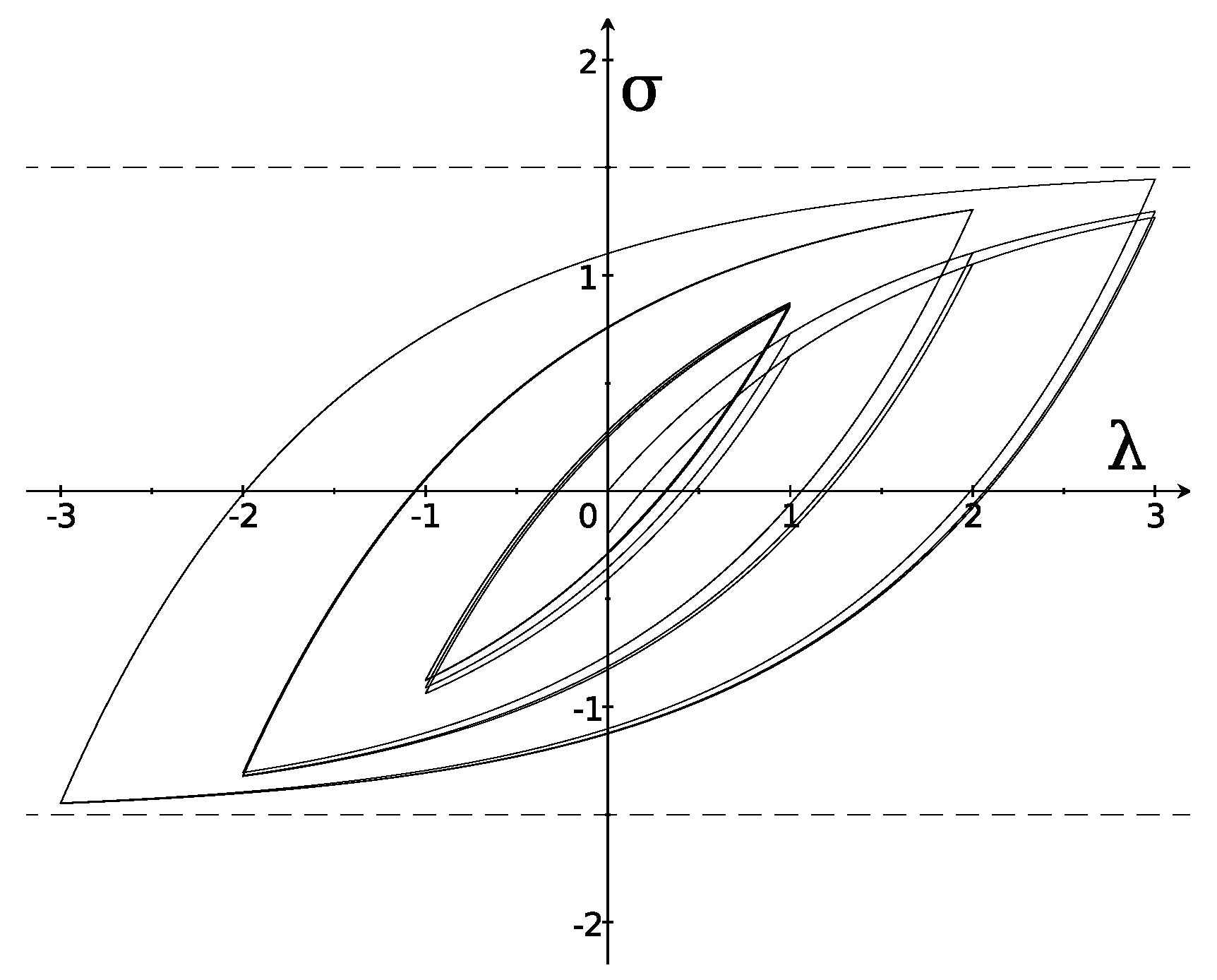
We start with a model based on a constant elastic differential stiffness $\alpha$. Let $\mathcal{G}\left(\lambda \right)=0$ so that $\Psi ={\sigma }^2/2\alpha$ and ${\chi }_1=\alpha$. The hysteretic function ${\gamma }_0$ is taken in the form

$${\gamma }_0\left(\sigma \right)=\frac{{\sigma }^2}{{\sigma }_u},{\sigma }_u>0.$$

Hence, the whole differential stiffness is

$$\frac{d\sigma }{d\lambda }=\frac{\alpha }{{\sigma }_u}({\sigma }_u-\sigma \mathrm{sgn}\dot{\lambda }).$$

(55)

In this event it follows that

$$\frac{d}{d\lambda }{(\sigma -{\sigma }_u)}^2=2\frac{\alpha }{{\sigma }_u}(\sigma -{\sigma }_u)({\sigma }_u-\sigma \mathrm{sgn}\dot{\lambda }),$$

where

$$\frac{d}{d\lambda }{(\sigma -{\sigma }_u)}^2=(2\alpha /{\sigma }_u)\{\begin{array}{cc}-{(\sigma -{\sigma }_u)}^2\hfill & \mathrm{if}\dot{\lambda }>0,\hfill \\ {\sigma }^2-{\sigma }_u^2\hfill & \mathrm{if}\dot{\lambda }<0.\hfill \end{array}$$

Thus,

$$\frac{d}{d\lambda }{(\sigma -{\sigma }_u)}^2\le 0$$

and the hysteresis loops are confined to the strip $\left|\sigma \right|\le {\sigma }_u$.

The hysteresis loops in Figure 1 are obtained by solving the system (54) and using (55) with $\alpha =1$ and ${\sigma }_u=1.5$.

• Plastic flow with a nonlinear elastic function.

Let

$$\mathcal{G}\left(\lambda \right)=tanh\left(\kappa \lambda \right),\kappa >0$$

and

$${\gamma }_0=\frac{1}{\beta }{\{\sigma -tanh\left(\kappa \lambda \right)\}}^2,\beta >0.$$

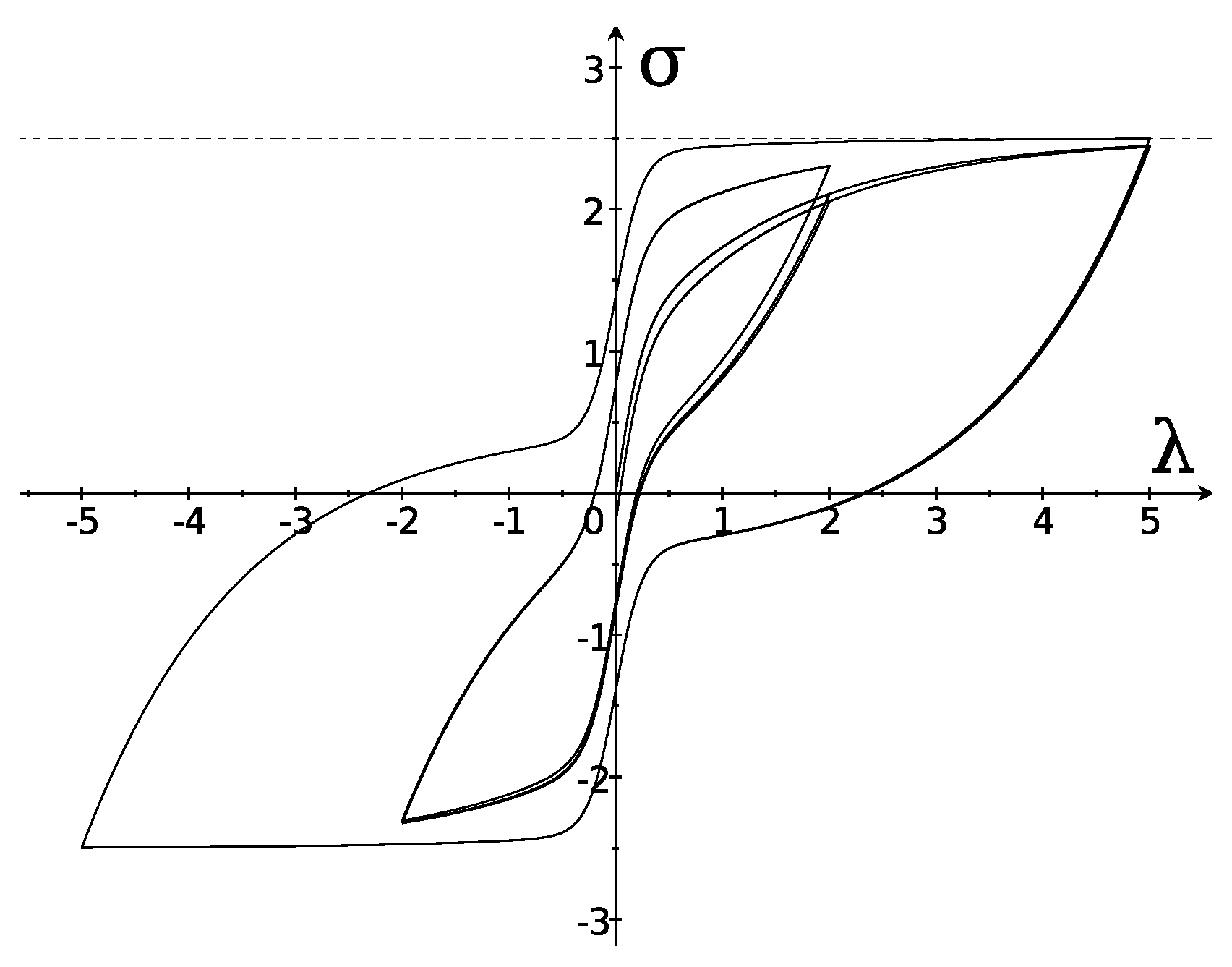
Hence, by (53) and (52) it follows that

$$\Psi (\sigma ,\lambda )=\frac{1}{2\alpha }{[\sigma -tanh\left(\kappa \lambda \right)]}^2+\frac{1}{\kappa }ln[cosh\left(\kappa \lambda \right)],$$

$${\chi }_1=\kappa [1-{tanh}^2\left(\kappa \lambda \right)],{\chi }_2=-\alpha [\sigma -tanh\left(\kappa \lambda \right)]\mathrm{sgn}\dot{\lambda }.$$

The differential stiffness $d\sigma /d\lambda$ can be given the form

$$\frac{d\sigma }{d\lambda }=\kappa [1-{tanh}^2\left(\kappa \lambda \right)]+\frac{\alpha }{\beta }\{\beta -[\sigma -tanh\left(\kappa \lambda \right)]\mathrm{sgn}\dot{\lambda }\}.$$

(56)

The hysteresis loops in Figure 2 are obtained by solving the system (54) and using (56) with $\alpha =1$, $\beta =1.5$, and $\kappa =4$. They well describe the hysteretic responses of lateral loads with respect to lateral displacements in a typical medium-rise building model (see, e.g., [20]).

• Elastic–plastic model.

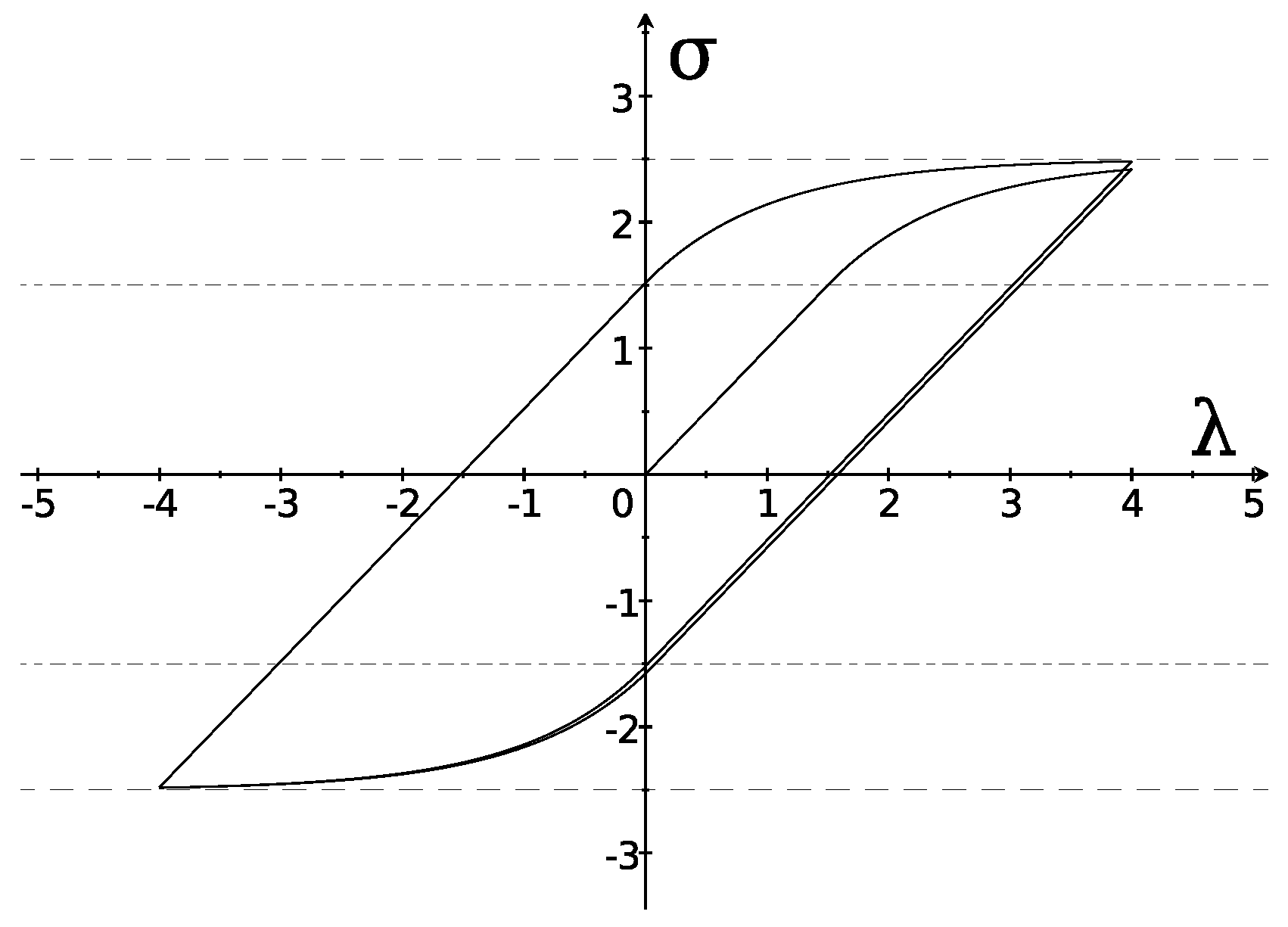
We now describe a solid undergoing linear behavior in the elastic regime. Hence, we let $\mathcal{G}\left(\lambda \right)=0$ and obtain

$$\Psi =\frac{{\sigma }^2}{2\alpha },{\chi }_1=\alpha .$$

To characterize $\gamma$ we consider two stress levels, ${\sigma }_u>{\sigma }_y>0$, and assume hysteretic effects are confined to the region $\left|\sigma \right|\in [{\sigma }_y,{\sigma }_u]$ in the form

$${\gamma }_0(\sigma ,\mathrm{sgn}\dot{\lambda })=\{\begin{array}{ccc}\left(\right|\sigma |-{\sigma }_y)/({\sigma }_u-{\sigma }_y)\left|\sigma \right|\hfill & \mathrm{if}\left|\sigma \right|\ge {\sigma }_y\hfill & \mathrm{and}\sigma \dot{\lambda }>0,\hfill \\ 0\hfill & \mathrm{if}\left|\sigma \right|<{\sigma }_y\hfill & \mathrm{or}\left|\sigma \right|\ge {\sigma }_y,\sigma \dot{\lambda }<0.\hfill \end{array}$$

The differential stiffness takes the form

$$\frac{d\sigma }{d\lambda }=\{\begin{array}{ccc}\alpha ({\sigma }_u-\left|\sigma \right|)/({\sigma }_u-{\sigma }_y)\hfill & \mathrm{if}\left|\sigma \right|\ge {\sigma }_y\hfill & \mathrm{and}\sigma \dot{\lambda }>0,\hfill \\ 0\hfill & \mathrm{if}\left|\sigma \right|<{\sigma }_y\hfill & \mathrm{or}\left|\sigma \right|\ge {\sigma }_y,\sigma \dot{\lambda }<0.\hfill \end{array}$$

(57)

Figure 3 shows the hysteresis loop obtained by solving the system (54) and using (57) with the parameters $\alpha =1$, ${\sigma }_u=2.5$, and ${\sigma }_y=1.5$. Within the region ${\sigma }_y\le \left|\sigma \right|\le {\sigma }_u$, the material behaves elastically during unloading and plastically during loading.

As exemplified by the previous models of plastic materials, the hysteretic properties are represented in simple and direct ways by an appropriate form of the entropy production $\gamma$ as a constitutive function. Analogous properties hold in the modeling of ferroics. In addition to the conceptual character of $\gamma$ as a constitutive function, these examples prove the experimental evidence of the reported method on the exploitation of the entropy inequality.

7. Conclusions

This paper deals with the mathematical formulation and the use of the second law of thermodynamics in continuum physics. Conceptually the second law states that the rate of entropy in any sub-region of the continuum is greater than the external entropy supply. This amounts to the assumption that the (rate of) entropy production is non-negative. Mathematically, this leads to a procedure for the selection of physically admissible constitutive properties [21]. In the Coleman–Noll formulation, the entropy flux, say $\mathbf{j}$, is $\mathbf{q}/\theta$, while $\mathbf{j}$ is a constitutive function in the Müller formulation. It is an important point of the present formulation that the entropy production $\gamma$ is also a constitutive function (Section 3).

The constitutive property of $\gamma$ is shown to have remarkable consequences on the whole thermodynamic scheme. Though quite uncommon in the literature, Section 5 shows that the aging properties of non-dissipative materials, that is, terms related to energy functions, result in positive entropy productions. Next, as is shown in Section 6, the occurrence of $\gamma$ as a constitutive function is essential in the modeling of thermodynamically consistent hysteretic materials. In particular, this is shown for elastic–plastic materials, though the analogue can be performed for magnetic or electric hysteresis [22,23,24].

It is a further result, shown in Section 6, that a representation formula allows a complete description of the consequences of the second law inequality. This greater generality is apparent when the constitutive equations involve vectors or tensors in rate-type equations.

From the standpoint of the mathematical modeling, the role played by the entropy production as a constitutive function is decisive, at least in the case of hysteretic materials. This is so because hysteresis exhibits a different behavior depending on the sign of a time derivative (namely, in loading and unloading). If, e.g., the variables are $\lambda ,\dot{\lambda }$, then the term ${\partial }_{\dot{\lambda }}\psi \ddot{\lambda }$ in the entropy inequality leads to ${\partial }_{\dot{\lambda }}\psi =0$. Hence, the dependence on $\dot{\lambda }$ happens through ${\partial }_{\lambda }\psi \dot{\lambda }$. The dependence on the sign of $\dot{\lambda }$ is then allowed by letting $\gamma$ depend on $\dot{\lambda }$ through $|\dot{\lambda }|.$ By this approach, the thermodynamic requirement results in a hysteretic Duhem-like model [25].

The procedure of Section 6, based on the constitutive function of entropy production, is likely to apply to hysteresis processes [26,27]. To our mind, a rate equation similar to (50) might well describe the time evolution of entropy–temperature loops.