Abstract
Lignocellulosic fibers are widely applied as reinforcement in polymer composites due to their properties. The thermal degradation behavior governs the maximum temperature at which the fiber can be applied without significant mass loss. It is possible to determine this temperature using Thermogravimetric Analysis (TG). In particular, when curves are obtained at different heating rates, kinetic parameters can be determined by using Arrhenius-based equations, and more detailed characteristics of the material are obtained. However, every curve obtained at a distinct heating rate demands material, cost and time. Methods to predict thermogravimetric curves can be very useful in the materials science field, and in this sense, mathematical approaches are powerful tools, if well employed. For this reason, in the present study, thermogravimetric curves from curaua fiber were obtained at four different heating rates (5, 10, 20 and 40 °C·min−1) and Vyazovkin kinetic parameters were obtained using free available software. After, the experimental curves were fitted using an artificial neural network (ANN) approach followed by a Surface Response Methodology (SRM) aiming to obtain curves at any heating rate between the minimum and maximum experimental heating rates. Finally, Vyazovkin kinetic parameters were tested again, with the new predicted curves at the heating rates of 7, 15, 30 and 50 °C·min−1. Similar values of the kinetic parameters were obtained compared to the experimental ones. In conclusion, due to the capability to learn from the own data, ANN combined with SRM seems to be an excellent alternative to predict TG curves that do not test experimentally, opening the range of applications.
1. Introduction
Lignocellulosic fibers are versatile materials used in different applications. Their use englobes the entire fiber for reinforcement in composite materials [1,2], or the use of their derivatives (cellulose, hemicellulose or lignin) in particular applications as shape memory of lignin-rubber composites [3], to obtain nanocellulose [4], to reinforce expanded composites [5] or cellulose biomedical applications [6], for example. This wide potential of application can be attributed to the great variety of chemical components (cellulose, hemicellulose, lignin, waxes, low molecular weight components, oil and others) presented in the lignocellulosic fibers [7,8]. In addition, the same fiber can have different properties depending on the plant age, climate, soil, among others [9].
Yao et al. [10] studied the thermal degradation behavior of 10 different lignocellulosic fibers, focusing on the Arrhenius kinetic parameters. The activation energy as a function of conversion presented similar values, independently of the chemical content of the fiber studied. A linear dependency in the conversion range α = 0.2–0.8 was observed for all fibers with an average apparent activation energy of 160–170 kJ·mol−1 for most of the fibers studied. Sunphorka et al. [11] studied an artificial neural network (ANN) model using 150 data from different lignocellulosic fibers in relation to Arrhenius kinetic parameters. The main results indicated that cellulose played a major role in the pre-exponential factor while the hemicellulose on the reaction order. According to the authors, all components affected the activation energy. Ornaghi Jr. et al. [7] studied the kinetic mechanisms involved in the thermal degradation of lignocellulosic fibers based on the chemical composition. The main results indicated that the activation energy of the fibers followed similar values to the cellulose component and that the thermogravimetric curves followed a similar pattern, independently of the chemical composition. Monticeli et al. [12] studied an ANN approach for lignocellulosic fibers using thermogravimetric analysis. The results indicated 50–60 as the optimal number of training datasets for all fibers. In addition, a reliable prediction of TG curves was obtained at different heating rates did not obtain experimentally.
Most of the fibers found in the literature follow a similar curve format, independently of the amount of the chemical components that indicate that the degradation process may follow specific degradation rules. For example, a mass loss of 5–10% is obtained at 100 °C due to moisture evaporation and, from 300 °C, the degradation of cellulose occurs. In some cases, a shoulder is observed at DTG (derivative thermogravimetric analysis) due to the higher amount of hemicellulose in a small range before cellulose degradation [13,14]. Hence, the thermogravimetric curves prediction of a particular lignocellulosic fiber can be extended to most of the fibers due to these similarities.
The main objective of this study is to perform the thermal degradation kinetic behavior of curaua fiber using the Vyazovkin kinetic method and ANN approach. The experimental curves were kinetically tested and curves that did not test experimentally were predicted, and new kinetic tests were carried out. The results presented reliable and robust data without the necessity of further experimental curves.
2. Materials and Methods
Curaua fiber received from CEAPAC (support center for community action projects) was used in this study. More details about the fiber characteristics can be found on [15,16].
Thermogravimetric analysis was carried out in a TA instrument model TGA-50 Shimadzu (Caxias do Sul, Brazil), under nitrogen atmosphere (50 mL·min−1), from 25 to 900 °C, using ~10 mg of each sample at four distinct heating rates (5, 10, 20 and 40 °C·min−1). The theoretical and predicted curves were used to calculate the kinetic parameters according to the Vyazovkin method. The calculation was carried out using the software developed by Drozin et al. [17]. A previous study Monticeli et al. [12] was used as a base for the obtaining of the new ANN curves at distinct heating rates. The predicted curves were used to calculate the kinetic parameters again and compare the results.
2.1. Kinetic Approach
The thermal degradation kinetic of lignocellulosic fibers follows the kinetics of the reaction of solids, in Equation (1):
where is the degradation rate, is the rate constant and is a conversion function.
The degradation kinetic follows Arrhenius’ equation (Equation (2)) and the heating rate changes linearly with temperature (Equation (3)):
where is the pre-exponential factor, is the activation energy, is the gas constant, is the temperature, is the heating rate and is the temperature in function of time.
The reaction model follows Equation (4) that expresses the function in the Equation (1) in a more analytical form:
where , and p are constants that represent a number of different reaction models. The characteristic conversion (α) vs. time plot is often reduced to three main types (accelerating, decelerating and sigmoidal). The equation above is a convenient mathematical approximation of the majority of possible mechanisms. For example, if the data obtained present m and n values higher than zero (0) and not presents a p value, the most probable mechanism is the diffusion one. Different combinations are referred to different mechanisms. More details can be found on [18,19,20,21].
In combining Equations (1)–(4) we obtain Equation (5):
The kinetic calculation was performed with the help of the Software developed by Drozin et al. [17] with the experimental and predicted curves.
2.2. Artificial Neural Network (ANN)
The ANN is conventionally constructed with three layers, i.e., an input, an output and a hidden layer. Each layer has different numbers of neuronal elements. In the present case, we use as input vectors a set of iTG curves at different heating rates. In this sense, the network will modify the weight of the interconnections between neurons in order to reproduce the given parameters. Figure 1 shows the scheme of the calculation process.
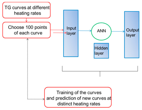
Figure 1.
Flowchart of the calculation process.
The main issues necessary to be defined before using the networks are the quality and number of the initial TG curves, the training algorithm and the number of neurons in the hidden layer. The number of initial TG curves used for the training should not be excessively large to avoid the over-training of the network, and it must be distributed correctly, in the sense that it usually appropriate to avoid sets of input vectors with the same output vectors. These kinds of orthogonal combinations produce better results than using random sets of parameters [22]. The following conditions (Table 1) were used to training the ANN network.

Table 1.
Parameters used to perform the ANN fit.
With the network training, we can feed the network with different curves and predicted new curves. The main drawback is that the curves outside the lower and higher heating rate cannot be created due to the accumulation of errors [22,23].
2.3. Surface Response Methodology (SRM)
The SRM is a statistical approach for modeling and analyzing a process in which the response of interest is affected by various variables [12,24,25]. Equation (6) describes the degradation curve interaction among the combination of temperature and heating rate. In using this method, the statistical relevance is kept and the number of experiments can be reduced.
where Z represents the predicted response (i.e., degradation curve— (%)), xi and xj are variations parameter, in which i represents the -axis (temperature T (°C)) and j is the -axis (heating rate HR (°C·min−1)). 0 is the constant coefficient; i is the linear coefficient; and ij is the interaction coefficient.
3. Results and Discussion
Figure 2a,b showed the experimental thermogravimetric curves and the respective derivatives of curaua fiber at different heating rates. The curves maintained the same format, independently of the heating rate used; only shifting the curve to a higher temperature. Three visible main loss stages are visualized: (i) at around 100 °C, a mass loss of 5% can be mainly attributed to the evaporation of intrinsic moisture, (ii) at around 300 °C a more abrupt mass loss attributed mainly to hemicellulose that extends up to 350 °C and, (iii) from 350 °C to 400 °C the degradation of cellulose (the main component) in a narrower range, representing the main degradation stage. Lignin decomposes over different temperature ranges [7,26,27].
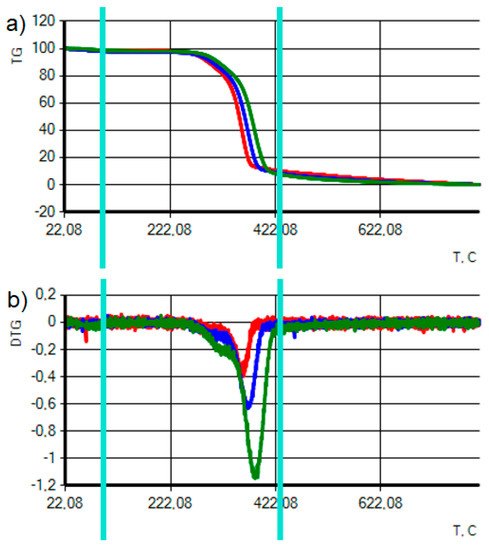
Figure 2.
(a) Thermogravimetric and (b) derivative TG curves of curaua fiber at different heating rates. The heating rates of 10, 20 and 40 °C·min−1 are represented by the red, blue and green lines. The vertical cyan lines represent the limit of calculation of the kinetic parameters.
All the curves above were used to calculate the kinetic parameters using the Vyazovkin kinetic model in the temperature range from 100 to 435 °C (main degradation stage). The corrected heating rates (provided by the Software) using the Vyazovkin method were 10.09, 20.1 and 39.79 °C·min−1. Figure 3a represents the activation energy in the conversion function and while Figure 3b the degradation rate in the function of conversion degree. An appropriate correlation between the theoretical and calculated degradation rate vs. alpha is obtained. The results presented the following values: Ea = 192.02 KJ·mol−1, A = 10.6 × 10¹⁵, m = 0.9, n = 1.71 and p = 0.
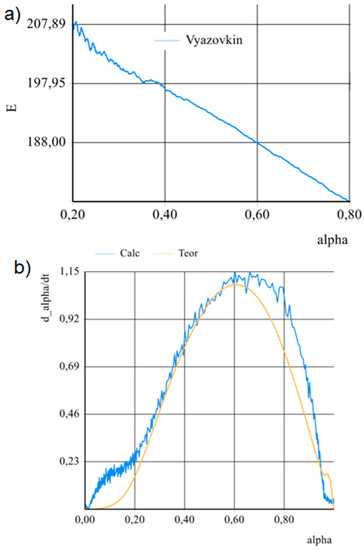
Figure 3.
Kinetic calculation of the experimental curves. (a) Activation energy in function of conversion degree and (b) degradation rate in function of conversion degree.
ANN prediction model is detailed in Section 2.2, in which the procedures used to calculate the predicted TGA fit are exhibited in Table 1. Using the same ANN parameters, this analysis can be reproduced for similar TGA curves through several neural network software (e.g., MatLab, OriginLab, CNTK, TFLearn, among others) [28].
Based on experimental degradation curves, the ANN fit was constructed with parameters variation, in which temperature and heating rate as the input parameters and the loss of mass (kinetic behavior) as output. The experimental dots were used to training the ANN. The number of training data influences the predictive curve, which was thoroughly investigated in previous work to optimize the ANN method [12]. Figure 4a presents the trained curves with the experimental ones, and Figure 4b exhibits the enlargement of initial degradation. An excellent fit was obtained for all heating rates tested. The coefficient of determination was R2 > 0.99 for all curves.
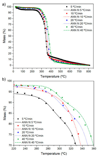
Figure 4.
(a) Thermogravimetric curves of curaua fiber at different heating rates trained using ANN approach according to Monticeli et al. [12], and (b) enlargement of initial degradation.
Only 1/10 of the experimental dataset has been used for training the ANN, resulting in a perfect fitting, resulting in an appropriate predictive result. Regarding the ANN application, new degradation behavior could be predicted with no need for long experiments [28].
From the ANN predicted curves, intermediate heating rates were predicted using the surface response methodology (SRM), resulting in a 3D Surface response to predict mass loss as a function of temperature and heating rate variation. Dot curves give the experimental data. The coefficient of determination R2 = 0.96 indicates the high reliability of predicted results. For the lowest heating rate (i.e., 5 °C/min), the degradation curve initiates at the lowest temperature for onset and endset, resulting in the slowest degradation of the remaining residue (15%), between 375–810 °C. At higher heating rates, more abrupt degradation occurs, increasing the onset and endset temperatures.
A well-trained ANN could develop a degradation mechanistic understanding of the natural fiber considered, considering that the ANN method is a purely phenomenological approach that can give accurate predictions [29]. For a better approximation of the theoretical and experimental results, the equation of the three-dimensional curve in Figure 5 was divided into three, presented in Equation (7)—for the temperature range of 25–250 °C, Equation (8)—for the temperature range of 250–410 °C and Equation (9)—for the temperature range of 410–810 °C.
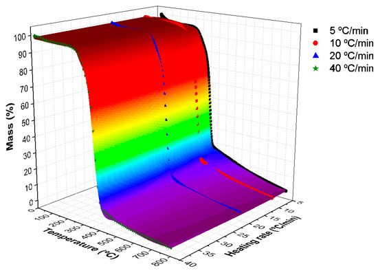
Figure 5.
Surface Response Methodology for the thermogravimetric curves.
The SRM curves (Equations (7)–(9)) were generated through a mathematical calculation of a three-dimensional regression plot of the second-order Equation (8). For error reduction and better compatibility with the complex curve presented in this work, the degradation curve was divided into three: room temperature up to Tonset; Tonset to Tendset; and Tendset to the final temperature, according to the procedure presented in reference [12].
Following SRM results, Figure 6 exhibits the predicted values of the thermogravimetric curves of curaua fiber using the heating rates of 7, 15, 30 and 50 °C·min−1. Through the ANN and SRM combination, it is possible to predict other degradation curves with different analysis parameters not accessed experimentally, decreasing costs and time related to tests repetitions with high reliability.
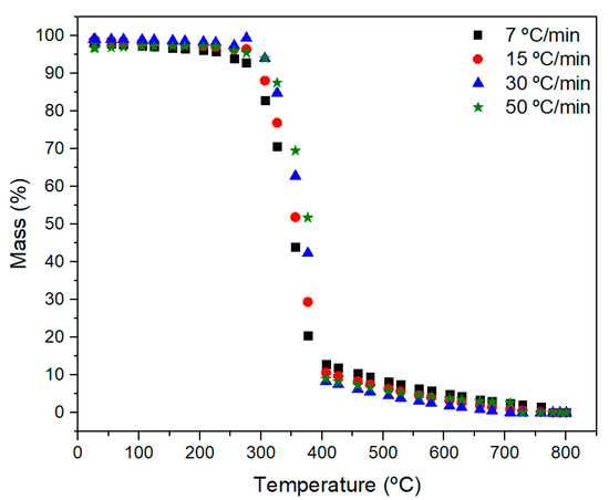
Figure 6.
Predicted thermogravimetric curves of curaua fiber.
The new kinetic parameters were caried out using the curves predicted (a) 7, 15 and 30 °C·min−1 and (b) 7, 15, 30 and 50 °C·min−1. The results presented the following values for condition (a): Ea = 228.74 KJ·mol−1, A = 3.59 × 10¹⁹, m = 0.1, n = 1.00 and p = 0 and for condition (b): Ea = 226.92 KJ·mol−1, A = 6.92 × 10¹⁸, m = 0.1, n = 1.53 and p = 0.
The values obtained, mainly the activation energy, are close to the experimental curves. The extrapolated curve (at 50 °C·min−1) used in condition b was also obtained. Of course, that the extrapolation of data using ANN is not well recommended due to the accumulation of errors. However, it can be used carefully and seems to work if the behavior did not change drastically from the previous behavior.
To confirm the ANN and SRM predicted methodology through the experimental data, the analysis of variance method was applied to evaluate the statistical influence of the heating rate variation on the Ea and A values, as shown in Table 2. The results confirmed that the Ea and A are directly proportional to the heating rate fluctuation since in both cases F > Fcritical and p-value < 0.05, confirming that there is a significant difference between experimental and predicted values. In addition, the percentage of contribution (PC) shows that error presented less influence on degradation kinetics parameters. This means that even with a slight variation on activation energy and pre-exponential factor, the use of different heating rate values has a high level of contribution in the determination of kinetic degradation parameters.

Table 2.
Analysis of variance results.
As a matter of fact, the t-test exhibits a p-value = 0.10, which is higher than 0.05. This result indicated that the experimental value presents no significative divergency than predicted values (true null hypothesis).
4. Conclusions
The present study proposed obtaining new thermogravimetric curves for curaua fiber at any heating rate between the minimum and maximum heating rates experimentally tested. For this, an Artificial Neural Network (ANN) followed by the Surface Response Methodology (SRM) was used to obtain new TG curves. Vyazovkin kinetic method was used in the experimental curves and in the newly obtained curves. The kinetic results presented similar values for the experimental and predicted curves, confirmed by statistical analysis. This approach can be extended to any material to obtain properties, parameters or to optimize processes.
Author Contributions
Conceptualization, H.L.O.J.; formal analysis, H.L.O.J.; investigation, H.L.O.J., F.M.M. and R.M.N.; methodology: H.L.O.J., F.M.M. and R.M.N.; Supervision, H.L.O.J.; writing—original draft, H.L.O.J.; writing—review and editing: F.M.M. and R.M.N. All authors have read and agreed to the published version of the manuscript.
Funding
This research received no external funding.
Institutional Review Board Statement
Not applicable.
Informed Consent Statement
Not applicable.
Data Availability Statement
Not applicable.
Conflicts of Interest
The authors declare no conflict of interest.
References
- Angrizani, C.C.; Ornaghi, H.L., Jr.; Zattera, A.J.; Amico, S.C. Thermal and Mechanical Investigation of Interlaminate Glass/Curaua Hybrid Polymer Composites. J. Nat. Fibers 2017, 14, 271–277. [Google Scholar] [CrossRef]
- Silva, H.S.P.; Ornaghi, H.L., Jr.; Almeida, J.H.S., Jr.; Zattera, A.J.; Amico, S.C. Mechanical Behavior and Correlation between Dynamic Fragility and Dynamic Mechanical Properties of Curaua Fiber Composites. Polym. Compos. 2014, 35, 1078–1086. [Google Scholar] [CrossRef]
- Nguyen, N.A.; Meek, K.M.; Bowland, C.C.; Naskar, A.K. Data of thermally active lignin-linkages and shape memory of lignin-rubber composites. Data Br. 2019, 22, 392–399. [Google Scholar] [CrossRef]
- Neves, R.M.; Lopes, K.S.; Zimmermann, M.G.V.; Poletto, M.; Zattera, A.J. Cellulose Nanowhiskers Extracted from Tempo-Oxidized Curaua Fibers. J. Nat. Fibers 2019, 17, 1355–1365. [Google Scholar] [CrossRef]
- Neves, R.M.; Lopes, K.S.; Lazzari, L.K.; Monticeli, F.M.; Zattera, A.J. Characterization of expanded polystyrene and its composites by supercritical carbon dioxide foaming approach. J. Porous. Mater. 2021. [Google Scholar] [CrossRef]
- Seddiqi, H.; Oliaei, E.; Honarkar, H.; Jin, J.; Geonzon, L.C.; Bacabac, R.G.; Nulend, J.K. Cellulose and its derivatives: Towards biomedical applications. Cellulose 2021, 28, 1893–1931. [Google Scholar] [CrossRef]
- Ornaghi, H.L., Jr.; Ornaghi, F.G.; Neves, R.M.; Monticeli, F.M.; Bianchi, O. Mechanisms involved in thermal degradation of lignocellulosic fibers: A survey based on chemical composition. Cellulose 2020, 4949–4961. [Google Scholar] [CrossRef]
- Yang, J.; Ching, Y.C.; Chuah, C.H. Applications of lignocellulosic fibers and lignin in bioplastics: A review. Polymers 2019, 11, 751. [Google Scholar] [CrossRef] [Green Version]
- Abdul, H.P.S.A.; Hossain, M.S.; Rosamah, E.; Azli, N.A.; Saddon, N.; Davoudpoura, Y.; Islam, N.; Dungani, R. The role of soil properties and it’s interaction towards quality plant fiber: A review. Renew. Sustain. Energy Rev. 2015, 43, 1006–1015. [Google Scholar] [CrossRef]
- Yao, F.; Wu, Q.; Lei, Y.; Guo, W.; Xu, Y. Thermal decomposition kinetics of natural fibers: Activation energy with dynamic thermogravimetric analysis. Polym. Degrad. Stab. 2008, 93, 90–98. [Google Scholar] [CrossRef]
- Sunphorka, S.; Chalermsinsuwan, B.; Piumsomboon, P. Artificial neural network model for the prediction of kinetic parameters of biomass pyrolysis from its constituents. Fuel 2017, 193, 142–158. [Google Scholar] [CrossRef]
- Monticeli, F.M.; Neves, R.M.; Ornaghi, H.L., Jr. Using an artificial neural network (ANN) for prediction of thermal degradation from kinetics parameters of vegetable fibers. Cellulose 2021, 28, 1961–1971. [Google Scholar] [CrossRef]
- Asim, M.; Paridah, M.T.; Chandrasekar, M.; Shahroze, R.M.; Jawaid, M.; Nasir, M.; Siekeng, R. Thermal stability of natural fibers and their polymer composites. Iran. Polym. J. 2020, 29, 625–648. [Google Scholar] [CrossRef]
- Monteiro, S.N.; Calado, V.; Margem, F.M.; Rodriguez, R.J.S. Thermogravimetric stability behavior of less common lignocellulosic fibers—A review. J. Mater. Res. Technol. 2012, 1, 189–199. [Google Scholar] [CrossRef] [Green Version]
- Ornaghi, H.L., Jr.; Zattera, A.J.; Amico, S.C. Thermal behavior and the compensation effect of vegetal fibers. Cellulose 2014, 21, 189–201. [Google Scholar] [CrossRef]
- Neves, R.M.; Lopes, K.S.; Zimmermann, M.G.V.; Poletto, M.; Zattera, A.J. Characterization of polystyrene nanocomposites and expanded nanocomposites reinforced with cellulose nanofibers and nanocrystals. Cellulose 2019, 26, 4417–4429. [Google Scholar] [CrossRef]
- Drozin, D.; Sozykin, S.; Ivanova, N.; Olenchikova, T.; Krupnova, T.; Krupina, N.; Avdin, V. Kinetic calculation: Software tool for determining the kinetic parameters of the thermal decomposition process using the Vyazovkin Method. SoftwareX 2020, 11, 100359. [Google Scholar] [CrossRef]
- Vyazovkin, S.; Burnham, A.K.; Criado, J.M.; Pérez-Maqueda, L.A.; Popescu, C.; Sbirrazzuoli, N. ICTAC Kinetics Committee recommendations for collecting experimental thermal analysis data for kinetic computations. Thermochim. Acta. 2011, 590, 1–23. [Google Scholar] [CrossRef]
- Šesták, J.; Berggren, G. Study of the kinetics of the mechanism of solid-state reactions at increasing temperatures. Thermochim. Acta 1971, 3, 1–12. [Google Scholar] [CrossRef]
- Vyazovkin, S.V.; Lesnikovich, A.I. Practical application of isoconversional methods. Thermochim. Acta 1992, 203, 177–185. [Google Scholar] [CrossRef]
- Vyazovkin, S. Evaluation of activation energy of thermally stimulated solid-state reactions under arbitrary variation of temperature. J. Comput. Chem. 1997, 18, 393–402. [Google Scholar] [CrossRef]
- Schmidhuber, J. Deep Learning in neural networks: An overview. Neural. Netw. 2015, 61, 85–117. [Google Scholar] [CrossRef] [Green Version]
- Agnol, L.D.; Ornaghi, H.L., Jr.; Monticeli, M.F.; Dias, F.T.G.; Bianchi, O. Polyurethanes synthetized with polyols of distinct molar masses: Use of the artificial neural network for prediction of degree of polymerization. Polym. Eng. Sci. 2021, 61, 1810–1818. [Google Scholar] [CrossRef]
- Debnath, S.; Reddy, M.M.; Yi, Q.S. Influence of cutting fluid conditions and cutting parameters on surface roughness and tool wear in turning process using Taguchi method. Meas. J. Int. Meas. Confed. 2016, 78, 111–119. [Google Scholar] [CrossRef]
- Aydar, A.Y. Utilization of Response Surface Methodology in Optimization of Extraction of Plant Materials. Stat. Approaches Emphas. Des. Exp. Appl. Chem. Process. 2018. [Google Scholar] [CrossRef] [Green Version]
- Patwardhan, P.R.; Brown, R.C.; Shanks, B.H. Understanding the fast pyrolysis of lignin. ChemSusChem 2011, 4, 1629–1636. [Google Scholar] [CrossRef] [PubMed]
- Cabeza, A.; Sobrón, F.; Yedro, F.M.; García-Serna, J. Autocatalytic kinetic model for thermogravimetric analysis and composition estimation of biomass and polymeric fractions. Fuel 2015, 148, 212–225. [Google Scholar] [CrossRef] [Green Version]
- Fernández-Fdz, D.; López-Puente, J.; Zaera, R. Prediction of the behaviour of CFRPs against high-velocity impact of solids employing an artificial neural network methodology. Compos. Part A Appl. Sci. Manuf. 2008, 39, 989–996. [Google Scholar] [CrossRef] [Green Version]
- Muravyev, N.V.; Luciano, G.; Ornaghi, H.L., Jr.; Svoboda, R.; Vyazovkin, S. Artificial Neural Networks for Pyrolysis, Thermal Analysis, and Thermokinetic Studies:The Status Quo. Molecules 2021, 26, 3727. [Google Scholar] [CrossRef] [PubMed]
Publisher’s Note: MDPI stays neutral with regard to jurisdictional claims in published maps and institutional affiliations. |
© 2021 by the authors. Licensee MDPI, Basel, Switzerland. This article is an open access article distributed under the terms and conditions of the Creative Commons Attribution (CC BY) license (https://creativecommons.org/licenses/by/4.0/).