Predicting the Bandgap of Graphene Based on Machine Learning

Abstract

Over the past decade, two-dimensional materials have become a research hotspot in chemistry, physics, materials science, and electrical and optical engineering due to their excellent properties. Graphene is one of the earliest discovered 2D materials. The absence of a bandgap in pure graphene limits its application in digital electronics where switching behavior is essential. In the present study, researchers have proposed a variety of methods for tuning the graphene bandgap. Machine learning methodologies have demonstrated the capability to enhance the efficiency of materials research by automating the recording of characteristic parameters from the discovery and preparation of 2D materials, property calculations, and simulations, as well as by facilitating the extraction and summarization of governing principles. In this work, we use first principle calculations to build a dataset of graphene band gaps under various conditions, including the application of a perpendicular external electric field, nitrogen doping, and hydrogen atom adsorption. Support Vector Machine (SVM), Random Forest (RF), and Multi-Layer Perceptron (MLP) Regression were utilized to successfully predict the graphene bandgap, and the accuracy of the models was verified using first principles. Finally, the advantages and limitations of the three models were compared.

1. Introduction

The study of two-dimensional (2D) materials, which are crystalline systems consisting of only one or a few atomic layers in thickness, dates back to the late 20th century [1]. The initial theoretical inquiries into two-dimensional (2D) materials focused on the structural properties of exfoliated graphite [2]. However, in 2004, a significant advancement occurred when Andre Geim and Konstantin Novoselov at the University of Manchester successfully prepared monolayer graphene through mechanical exfoliation [3].

Pure Graphene is frequently regarded as a zero-bandgap material, a classification that signifies that the valence and conduction bands are tangent at the Dirac point, resulting in an energy gap that is considered to be zero. Consequently, graphene invariably manifests metallic or semi-metallic properties [4]. In conventional semiconductors, the absence of an applied voltage hinders electron mobility due to the presence of a bandgap. The application of a voltage enables electron conduction. Graphene’s intrinsic zero-bandgap property impedes the effective current “shutdown” necessary for field-effect transistors (FETs), resulting in switching ratios that frequently fall below 10 [5]. This limitation does not align with the demand for high switching ratios in digital logic circuits, significantly constraining the application of graphene in conventional semiconductors. This severely limits the direct application of graphene in conventional electronic devices. The study of the bandgap of graphene is of significant engineering and application value, as it directly relates to the viability of graphene for widespread use in practical electronic devices.

In recent years, researchers have made significant progress in tuning graphene’s bandgap using various methods. For example, applying a vertical electric field to bilayer graphene enables continuous bandgap modulation, reaching approximately 200–250 meV, as confirmed by infrared photoelectric measurements [6,7]. Building on this tunability and leveraging VO₂’s phase-transition properties, a dynamically tunable dual-frequency terahertz absorber based on graphene–VO₂ hybrid metamaterials has been proposed [8]. Similarly, graphene-based THz metamaterials have been designed as tunable 2-bit encoders, switches, and absorbers operating in the 1–4 THz range [9]. Asymmetric straining is one effective physical method to open a bandgap near the Dirac point, significantly altering graphene’s light absorption properties [10]. Chemical functionalization achieves similar results. Fully hydrogenated graphene undergoes sp² → sp³ hybridization, resulting in a wide bandgap of 3.5–4.0 eV [11], while perfluorination yields a bandgap of approximately 5.75 eV [12]. To preserve graphene’s high mobility, doping with heteroatoms such as boron or nitrogen typically tunes the bandgap within 0.1–0.5 eV [13]. Additionally, epitaxial growth on substrates like h-BN or SiC breaks sublattice symmetry and induces a modest 0.2–0.3 eV gap [14,15].

Experimental bandgap values are usually obtained via first-principles methods like density functional theory (DFT) [16,17]. However, these calculations are computationally intensive, often require supercomputing resources, and may carry data reliability concerns—making them less cost-effective for large-scale screening. By contrast, machine learning offers a more efficient alternative. In this work, we generate DFT datasets for single-layer graphene exposed to N-doping and hydrogenation, as well as AB-stacked bilayer graphene under vertical electric fields. We then train and compare Random Forest, Support Vector Regression, and Multilayer Perceptron models. The best-performing model achieves prediction errors of approximately 10%, demonstrating that machine learning can both accurately and rapidly predict graphene bandgaps.

2. Methods

2.1. Graphene Modeling

The electronic band gap is an intrinsic property of insulators and semiconductors that exerts a significant influence on the optical and transport properties of the material. It occupies a central role in the domain of modern device physics and technology. In this study, the initial step involves the modeling of graphene and doped graphene using Materials Studio 2023.

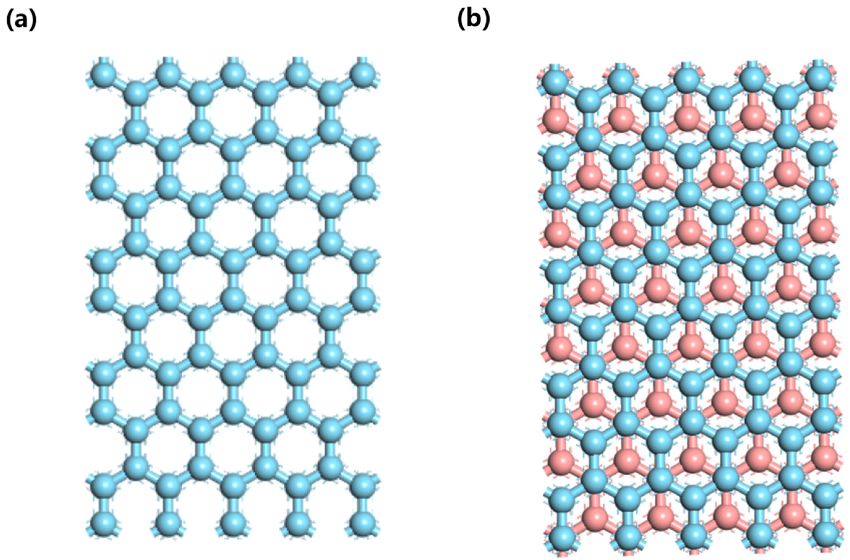
As detailed in

Table 1. Graphene structural parameters.

Structure	Methods/Å	Calculated/Å	Experimental/Å
Graphene	a	2.456	$2.460$[18]
	b	2.456	$2.460$[18]
AB-stacked	spacings	3.40	$3.35$[19]

, these computations were performed in accordance with the structural parameters reported by Baskin, Y., Meyer, L. [18], Lee, J.K., Lee, S.C., Ahn, J.P. [19], among others. The structural parameters provided in Table 1 are used to establish a 4 × 4 × 1 single-layer graphene and a 4 × 4 × 2 AB-stacked bilayer graphene in the Cartesian coordinate system. The lattice constants a1 and a2 (cf. Figure 1) are expressed in the Cartesian coordinate system as:

$$\mathrm{a}1=\mathrm{a}0\sqrt{2}(3,\sqrt{3})$$

$$\mathrm{a}2=\mathrm{a}0\sqrt{2}(3,-\sqrt{3})$$

where a₀ is the interatomic distance or C–C bond length and has been found to be close to 1.42 Å. Given that the periodic boundary condition (PBC) is generally employed in Materials Studio modeling, and that repetitive cells are present in the Z-axis direction of the relevant model, the thickness of the vacuum layer was set to 15 Å. This thickness is sufficient to prevent spurious interactions between the repetitive cells [20]. In this study, monolayer graphene is utilized as the target material to examine two external factors: the adsorption of H atoms and N doping. Conversely, bilayer graphene is employed as the target material to investigate the perpendicular external electric field.

2.1.1. Vertical External Electric Field with Bilayer Graphene

The addition of a layer to a single layer of graphene results in a significant alteration of the material’s structural configuration, thereby yielding a bilayer graphene. The most prevalent interlayer arrangements in bilayer and multilayer graphene are known as AB stacking and AA stacking, respectively. AB stacking is characterized by a minimal total energy and enhanced thermodynamic stability, a property attributable to the relative offset of carbon atoms between layers. In contrast, AA stacking can be regarded as a comparatively “sub-stable” structure, wherein the carbon atoms of the two layers are fully aligned. In this study, AB-stacked bilayer graphene is selected as the object of study, as illustrated in Figure 2b.

The Dmol3 module in the Materials studio has the capability to apply a perpendicular external electric field. Based on the experimental data, a vacuum layer of 3.4 Å was added to the surface of the 4 × 4 × 2 AB bilayer graphene to improve the accuracy and reliability of the study. An external electric field perpendicular to the bilayer graphene was applied through the built-in script of Dmol3. The following investigation will model bilayer graphene with an AB stacked structure under the influence of a perpendicular external electric field.

2.1.2. N-Doping with Monolayer Graphene

Doping is a conventional method of modulating material properties that has been demonstrated to be an effective means of inducing band gap opening in graphene. In the context of the periodic table, elements that are positioned in the same row as carbon are often utilized as substitution elements. In this study, the element nitrogen (N) is selected as the substitution element. N atoms, due to their nearly identical scale with carbon (C) atoms, form three carbon–nitrogen (C-N) bonds after interacting with C atoms through sp² hybridization. At this point, the planar lattice of monolayer graphene is almost undeformed, and some of the properties of graphene can be retained. However, the presence of N atoms disrupts the symmetry of the graphene sublattice, thereby inducing the formation of a band gap. The N-doped graphene isomers, which are formed through the selection of disparate doping positions, exhibit marked disparities in terms of stability, bond length, and band gap introduced. P. Rani and V. K. Jindal [20] have demonstrated that the electronic nature of the graphene lattice is contingent upon its symmetry. The positioning of dopant atoms, therefore, assumes a pivotal role in the regulation of the band gap. In the case that the dopant is situated in the same sublattice position (A or B) in the neighboring sublattice of graphene, the band gap attains its maximum value due to the combined effect of sublattice symmetry breaking. Conversely, when the dopant is located in the neighboring position (alternating sublattice position), the band gap closes.

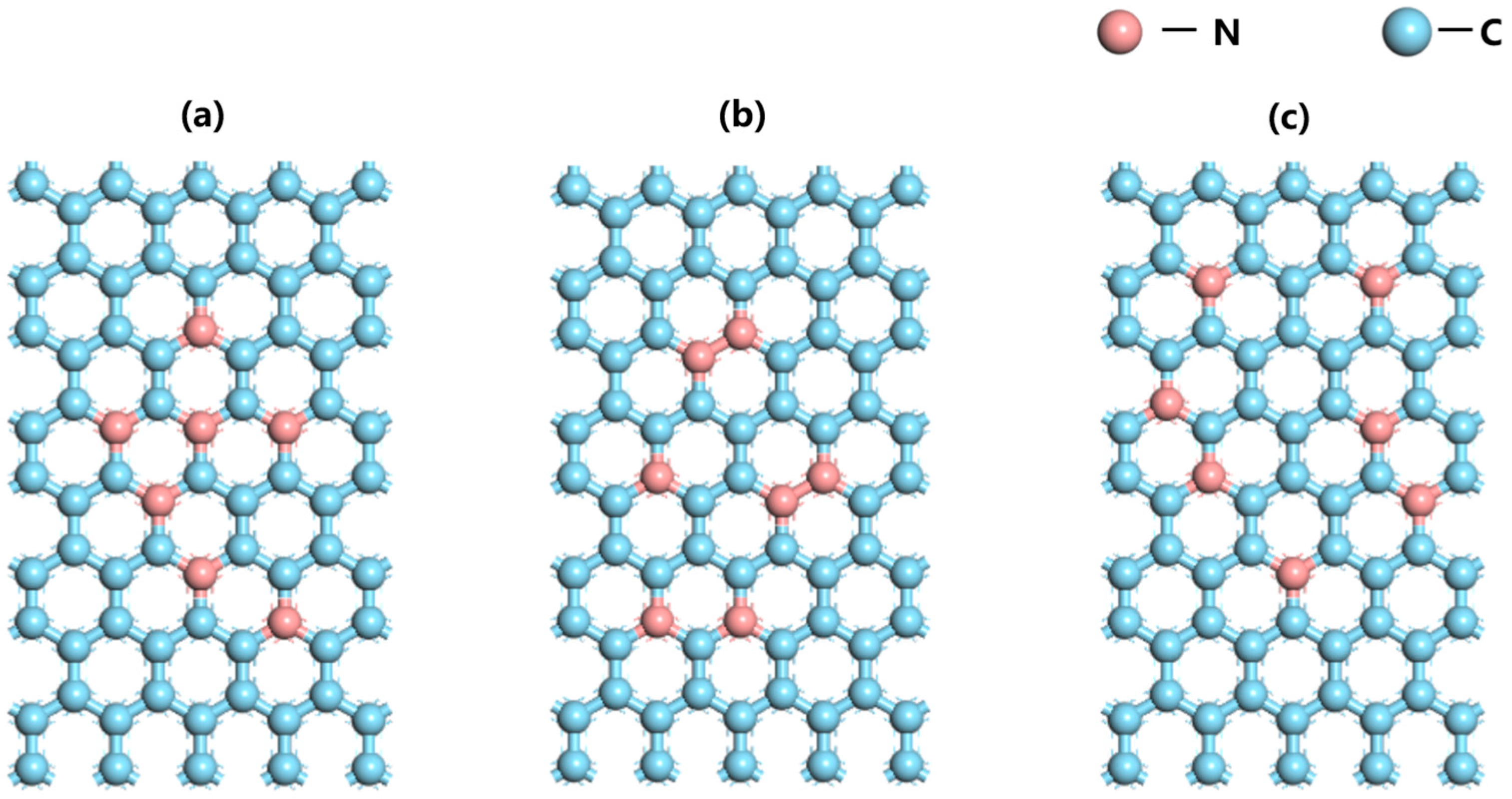
In this study, nitrogen (N) atoms are directly doped into monolayer graphene within a concentration range of 2% to 12%, based on the established 4 × 4 × 1 graphene structure. The incorporation of N atoms into graphene results in a spectrum of bandgaps, and for each doping concentration, 20 configurations are randomly generated to ensure that the bandgap differences attributable to different configurations can be adequately addressed. Figure 3 illustrates some of these configurations.

2.1.3. H Adsorption with Monolayer Graphene

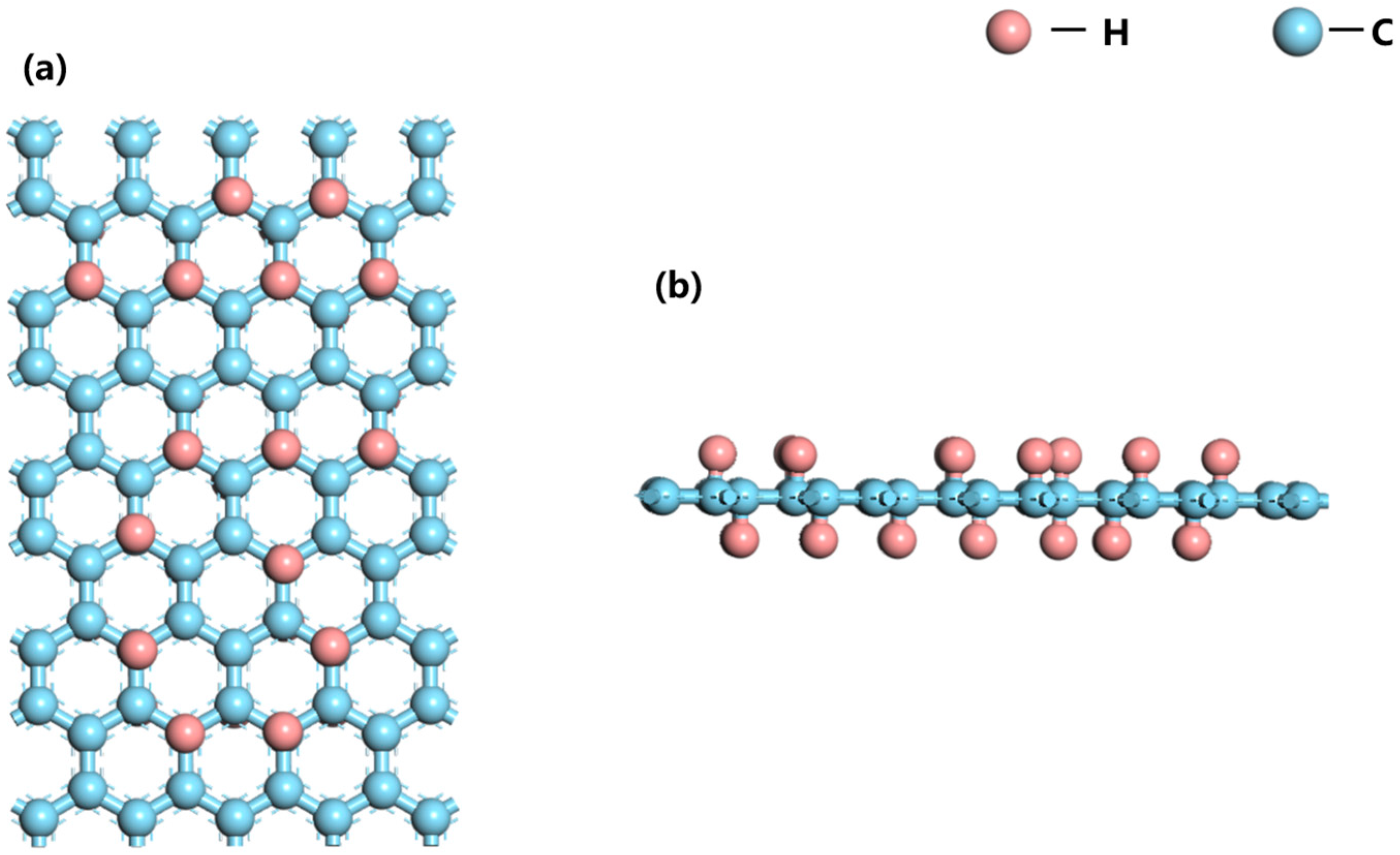
Fully hydrogenated graphene, also referred to as graphane, is a two-dimensional hydrocarbon. The C-C bonds in graphane exhibit the sp³ configuration. The crystal structure of graphane is a two-dimensional analog of cubic diamond because the chemical bonds are sp³ hybridized. Hydrogen atoms are bonded to carbon atoms on both sides of the plane in an alternating manner. In the various configurations with partially H-graphene, two are generally more stable. One of these is the chair conformation. In this configuration, hydrogen atoms in the two neighboring carbon atoms are located in the graphane plane of the top and bottom of the alternating direction. This makes the local carbon skeleton form a more stable “bending” structure. This structure has regular undulation in the 2D projection. It looks like a wave-like “chair” shape, as shown in Figure 4. The present study concentrates on the subject of graphene in relation to partially hydrogenated chairs.

The partially hydrogenated graphene conformation is constructed by removing hydrogen atoms from perfect graphene. The employment of graphene, which was of a relatively large size in the experiments, resulted in the formation of H vacancies. These vacancies, while distributed randomly on the main body of the graphene, exhibited the potential to organize into regular conformations. In this study, we examine the simplest case, in which H-atom pairs are removed from graphene at random. For each H coverage, configurations are randomly generated to ensure that the H-atom pairs are removed randomly, thereby facilitating further investigation of the band gap of graphene. Figure 4 illustrates the possible configurations of chair graphene at 39% adsorption rate.

2.2. Data Computation

Machine learning is predicated on data, and the process of model learning is contingent on the availability of substantial quantities of high-quality data, which is necessary for the extraction of laws and patterns. In this chapter, the optimization of graphene’s structural elements and the calculation of its electronic properties are executed through the utilization of Materials Studio software, which is founded on the principles of density functional theory.

The initial focus will be on the data for AB-stacked bilayer graphene with a vertical external electric field. However, it is essential to note that specific data calculations can only be performed after optimizing the cell structure at this particular point in time. This geometry optimization is addressed in the subsequent two discussions: one on N doping with single layer graphene band gap and the other on H atom adsorption with single layer graphene band gap. In the geometry optimization process, which is carried out using the Dmol3 module of the Materials Studio, the exchange correlation potentials between electrons are simulated by the Perdew–Burke–Ernzerhof (PBE) generalized function based on the generalized gradient approximation (GGA). It has been demonstrated that, in the absence of symmetry constraints, the systems are found to be fully relaxed. Through the implementation of an all-electronic treatment that incorporates d- and p-polarization functions, a 2 × 1 × 1 k-point lattice is employed for the purpose of structural optimization. The convergence of relaxation at the atomic positions is indicated by a change in the total energy less than 1 × 10⁻⁵ Ha/Å, in conjunction with a force on each atom less than 0.01 Ha/Å. The plane-wave cutoff energy was set to 400 eV. The Monkhorst–Pack scheme is used for sampling the Brillouin zone. This optimization setup is equally applicable when discussing the structural optimization of N-doped graphene and H-adsorbed graphene. Following the optimization of the bilayer graphene structure, the band gap values of graphene are calculated using the Dmol3 module. The external electric field magnitude is randomly selected between 0 eV/nm and 4 eV/nm, and the results of the DFT calculations by Yuanbo Zhang, Tsung-Ta Tang [21], and Wang Tao [22] are combined to create all the data sets, which total approximately 200 sets.

Subsequently, the discussion transitions to the analysis of N doping and the graphene band gap. The size of the graphene supercell is a determining factor in the potential rates of adsorption and doping. This principle also applies to the subsequent discussion of H atom adsorption. Theoretically, the larger the monolayer graphene, the higher the doping and adsorption rates it can accommodate. However, this study employs the first principles of calculating the bandgap of boron-doped graphene, which necessitates a greater computational time and renders the calculations more costly. In this study, a 4 × 4 × 1 single layer of graphene is utilized. In the modeling of graphene, the GGA-based PBE is employed as the exchange-correlation generalized function. For the purpose of geometry optimization, all internal coordinates undergo relaxation until the force on each atom is less than 0.005 Å. The remaining setup is consistent with the AB-stacked bilayer graphene, thereby ensuring the stability of the N atoms’ structure following doping of the graphene. Subsequent to the structural stability of N-doped graphene, the graphene band gap is calculated at this juncture. This calculation is performed using the Dmol3 module of Materials Studio. In conjunction with the calculations of P Rani and VK Jindal [20], approximately 150 sets of data are assembled.

The final calculation discusses the data between the band gaps of H atom adsorbed monolayer graphene. In accordance with the preceding discourse, this study employed the same 4 × 4 × 1 monolayer graphene. The configuration of graphene adsorbed by H at this particular juncture is determined by the random selection of the adsorption rate, as previously discussed. Additionally, five distinct conformations are taken into account at a constant adsorption rate. Following the establishment of the graphene structure and the subsequent part of crystal structure optimization, the exchange correlation generalization is employed as a simulation using the GGA-based PW91 parameterization. The remaining parameter settings are maintained at a consistent level with those implemented in the case of AB-stacked bilayer graphene. This ensures the stability of the crystal structure of the graphene after the adsorption of a hydrogen atom on the graphene at a specific rate. Subsequent to the structural stabilization of graphene by hydrogen atoms, the graphene band gap is computed by employing the Dmol3 module of Materials Studio. In conjunction with the findings of DFT calculations by Haili Gao, Lu Wang [23], and other researchers, the totality of the datasets comprises approximately 200 sets of data.

2.3. Machine Learning Model Settings

In this work, the utilization of Matlab 2023b is instrumental in the analysis of the prediction outcomes of machine learning algorithms, with the objective of assessing the band gap of graphene. Additionally, the work involves a comparative analysis of the prediction results derived from various machine learning algorithms.

Prior to the commencement of the study, the training set data was pre-processed using equal-width binning in order to observe the distribution of graphene bandgap values under differing external factors. As demonstrated in Figure 5, the distribution of the dataset is relatively stable, with a consistent number of samples in each interval.

In this study, the generation of the perpendicular external electric field with AB stacked bilayer graphene bandgap, N doping with monolayer graphene bandgap, and H adsorption with monolayer graphene bandgap will be computed using RF regression algorithm, SVM regression algorithm, and MLP regression algorithm, respectively. For each machine learning algorithm, there is a multitude of hyperparameters. For all datasets, this study employs a 7:1.5:1.5 ratio to divide the training set, test set, and validation set.

For each machine learning method, there are multiple hyperparameters, the selection of which is contingent on the size of the dataset, which in turn determines the range of possible values. The present study exclusively attempted to combine values from a single set. The Random Forest regression algorithm is the first of these. The most significant hyperparameters are the number of decision trees, the minimum number of samples in a leaf node, the depth of the tree, and the number of feature samples. The number of decision trees is indicative of the number of decision trees that have been trained in parallel within the forest. It is evident that as the number of trees increases, the variability of the model is known to decrease, thus resulting in more stable predictions. The minimum number of samples in a leaf node is equivalent to the minimum number of samples that should be included in a leaf node. This can limit the growth depth of the tree and prevent overfitting caused by overly small leaf nodes. It has been demonstrated that the greater the number of feature samples, the stronger the fitting ability of a single tree (smaller bias). The extent to which the dataset is partitioned is contingent upon the depth of the tree. When the sample size is 150, the random forest is configured with 50 trees, the minimum number of samples in a leaf node is set to 1, and only one feature is sampled per split, the model’s ability to fit and its subsequent generalisation performance are significantly improved. The specific values of the random forest algorithm’s hyperparameters are detailed in

Table 2. Random Forest Regression Algorithm Machine Learning Model Parameter Settings.

Hyperparameters	Values
Number of decision trees	50
Number of minimum leaf node samples	1
Number of feature samples	1
MaxNumSplits	5

and

Table 3. Support Vector Machine Regression Algorithm Machine Learning Model Parameter Settings.

Hyperparameters	Values
Regularization parameter C	400
Kernel function	Gaussian
Insensitive bandwidth	0.001

.

The second is the support vector machine regression algorithm, where the following hyperparameters are of particular significance: the regularisation parameter C, the kernel function type, and the insensitivity bandwidth ε. The regularisation parameter C serves as the upper bound for the Lagrange multiplier α in binary problems. The purpose of this procedure is to penalise sample errors that fall outside the interval range. It is evident that C exerts a direct influence on the number of points permitted to fall within the specified interval, or to be misclassified, in addition to the geometric interval. The selection of kernel function type is contingent upon the specific experimental requirements. In this study, the kernel function type was selected as the Gaussian kernel function. The significance of the insensitivity bandwidth (ε) is that the loss function does not calculate the loss for points with prediction errors smaller than ε. Instead, it only penalises errors exceeding ε. As ε increases, the insensitive interval widens, and more training points fall within the ε range without becoming support vectors. This results in a sparser and smoother model. Conversely, a decrease in ε results in a narrower bandwidth, more points falling within the penalty range, and a more optimal fit of the model to the data, though this is accompanied by an increased risk of overfitting. The hyperparameter settings for the support vector machine are therefore shown in Table 3.

In conclusion, it is evident that the multi-layer perceptron regression algorithm is characterised by a considerable number of hyperparameters. The size of the hidden layer has been shown to directly determine the network’s expressive capability and the number of parameters. It has been demonstrated that the maximum number of training iterations can be used to control the maximum training time and convergence timing. Furthermore, it has been shown that the learning rate affects the step size and convergence speed of each parameter update. Finally, based on the size of the dataset, the selection of hyperparameter combinations for the multi-layer perceptron regression algorithm is shown in Table 3 and

Table 4. Multilayer perceptron regression algorithm machine learning model parameterization.

Hyperparameters	Values
Maximum number of training rounds	500
Learning rate	0.01
Minimum gradient threshold	1 × 10−6
Hidden Layer Size	10

.

Subsequent to the implementation of the aforementioned machine learning algorithm with predefined hyperparameters, the objective function to be optimized in the training set is set to mean square error (MSE) in both the random forest regression algorithm and the multi-layer perceptron regression algorithm, as follows.

$$\mathrm{M}\mathrm{S}\mathrm{E}={\displaystyle \frac{1}{\mathrm{N}}}{\sum }_{\mathrm{i}=1}^{\mathrm{N}}{\left({\mathrm{y}}_{\mathrm{i}}-\widehat{{\mathrm{y}}_{\mathrm{i}}}\right)}^2,$$

(1)

In the context of random forest regression, the mean square error (MSE) is selected as a metric to assess the quality of the split, given its ability to identify features and cut-points that can minimize the leaf nodes while simultaneously weighting the average MSE. This approach enables the tree structure to reduce the prediction variance. Concurrently, the results are outputted by averaging the prediction results of each tree. In the sense of the squared error, the sample mean minimizes the overall mean-squared error (MSE). Furthermore, the MSE has a quadratic penalty effect on the large deviation points. This effect causes the algorithm to pay more attention to and correct the samples with large prediction errors. Consequently, the fitting accuracy can be further improved in the small-sample scenario of this experiment.

In the context of multilayer perceptron regression, the loss function is typically determined by the mean squared error (MSE) metric. This selection is primarily predicated on the fact that MSE is a smooth and derivable quadratic function. Consequently, it facilitates the efficient computation and update of network parameters in accordance with the back-propagation method and gradient descent. Additionally, when the output layer is a linear activation, MSE assumes a convex form in the parameter space of the layer. This property of MSE renders the optimization process smoother and facilitates convergence. Furthermore, MSE imposes a greater penalty on large error samples and can inherently correct large samples with significant errors. Furthermore, MSE imposes a more substantial penalty for substantial error samples, and it can be seamlessly integrated with L2 regularization to minimize error while regulating model complexity and enhancing generalization performance.

The objective function to be optimized in the support vector machine regression algorithm is as follows:

$${\displaystyle \frac{1}{2}}{‖w‖}^2+400{\sum }_{i=1}^{150}\left({\xi }_i+{\xi }_i^{*}\right),$$

(2)

The primary objective of the objective function ${\displaystyle \frac{1}{2}}{‖w‖}^2$ is to regulate the model’s intricacy, thereby ensuring the regression function’s optimal smoothness. This is paramount in the context of the study, as it is designed to prevent overfitting when the sample size is limited. The second loss term $400{\sum }_{i=1}^{150}\left({\xi }_i+{\xi }_i^{*}\right)$ is employed to penalize deviations between the predicted and true values that exceed the ε bandwidth. The regularization parameter C = 400 is set relatively high so that the machine learning model penalizes errors beyond ε = 0.001 to fit the data as accurately as possible, and the insensitive loss bandwidth allows the model to ignore small errors (i.e., those smaller than ε) and improve robustness to noise. The model is calibrated with a very small epsilon, set at 0.001, which renders it nearly intolerant to errors and well-suited for scenarios where noise is minimal and prediction accuracy is paramount. The kernel function employed is a Gaussian kernel function, a choice that is predicated on its superior nonlinear modeling capability. This capability enables the function to map inputs to a high-dimensional space, a task typically undertaken by a linear model when fitting nonlinear relationships. The Gaussian kernel’s capacity for smoothness and infinite-dimensional representation enables it to capture complex feature relationships in scenarios where the sample size is limited, while avoiding the overfitting that plagues the polynomial kernel.

Following the optimization of the objective function, the machine learning model must undergo evaluation to detect and rectify issues related to overfitting or underfitting as expeditiously as possible. The evaluation of the machine learning model will be carried out in the validation set and test set. The primary metric employed is the mean square error (MSE), which has been calculated above, to supervise the occurrence of outliers in the prediction results. The secondary metric considered is the mean absolute error (MAE). The coefficient of determination, denoted by R², is a metric of evaluation that is employed to assess the performance of a machine learning model in predicting the true value. The closer R² is to 1, the more effective the model is in its fit to the target function. The average distance between the predicted value and the true value directly reflects the performance of the model. The mathematical expression of the mean absolute error (MAE) and the coefficient of determination (R²) is as follows:

$$\mathrm{M}\mathrm{A}\mathrm{E}={\displaystyle \frac{1}{\mathrm{N}}}{\sum }_{\mathrm{i}=1}^{\mathrm{N}}\left|{\mathrm{y}}_{\mathrm{i}}-\widehat{{\mathrm{y}}_{\mathrm{i}}}\right|,$$

(3)

$${\mathrm{R}}^2=1-{\displaystyle \frac{{\sum }_{\mathrm{i}=1}^{\mathrm{N}}{\left({\mathrm{y}}_{\mathrm{i}}-\widehat{{\mathrm{y}}_{\mathrm{i}}}\right)}^2}{{\sum }_{\mathrm{i}=1}^{\mathrm{N}}{\left({\mathrm{y}}_{\mathrm{i}}-\overline{\mathrm{y}}\right)}^2}}$$

(4)

3. Results and Discussion

In this experiment, a range of machine learning models were utilized to predict the bandgap of graphene. The correlation between the theoretically calculated values and the machine learning predictions was then plotted. “The corresponding plots of vertical external electric field, N doping and H atom adsorption rate are shown in Figure 6a–c, Figure 7a–c, and Figure 8a–c, respectively.” The prediction results of the three graph species are shown below. The results are based on the test set and the machine learning models. The random forest (RF) model shows good prediction ability under all three influencing factors. Its data points are close to the diagonal line. This indicates that the predicted values are highly consistent with the true values. The model is stable and has strong generalization ability. In contrast, on the test set, the SVM algorithm and the MLP algorithm show a similar trend, with smaller prediction errors in the low bandgap region and larger errors in the high bandgap. The error is as high as 50%. For example, in Figure 8b, there exists a point where the computed bandgap value is 1.5 eV while the predicted bandgap value is about 3 eV, with an error of up to 50%. We believe that these errors come from two aspects: first, This particular instance constitutes a special case, and the remainder of the calculations are maintained within the standard range; second, there are fewer training samples in the high bandgap region, and the generalization ability is limited, which leads to a relatively large prediction error for these “tail samples”. The quantitative calculation of the generalization ability and specific error of the machine learning model can be further analyzed by the specific calculation of the mean squared error (MSE), the mean absolute error (MAE), and the coefficient of determination (R²) values in the subsequent section.

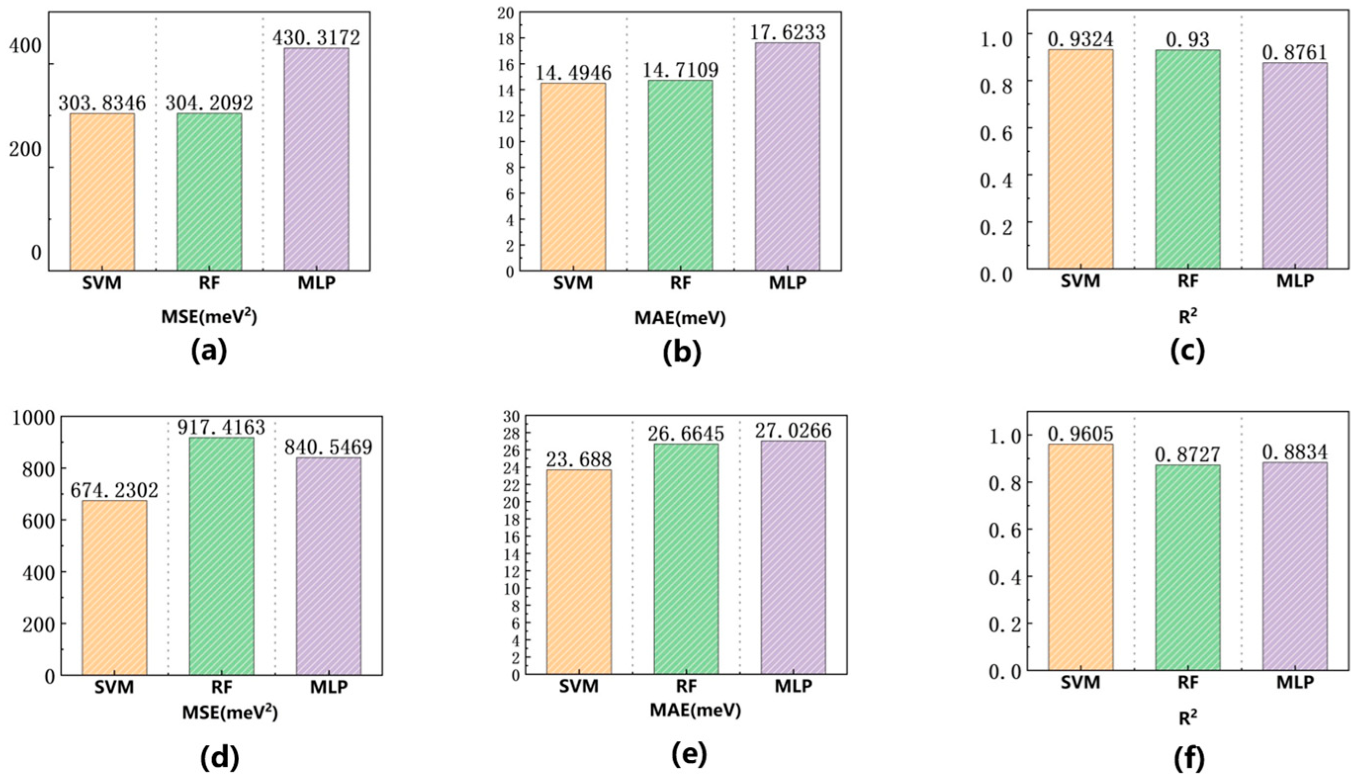
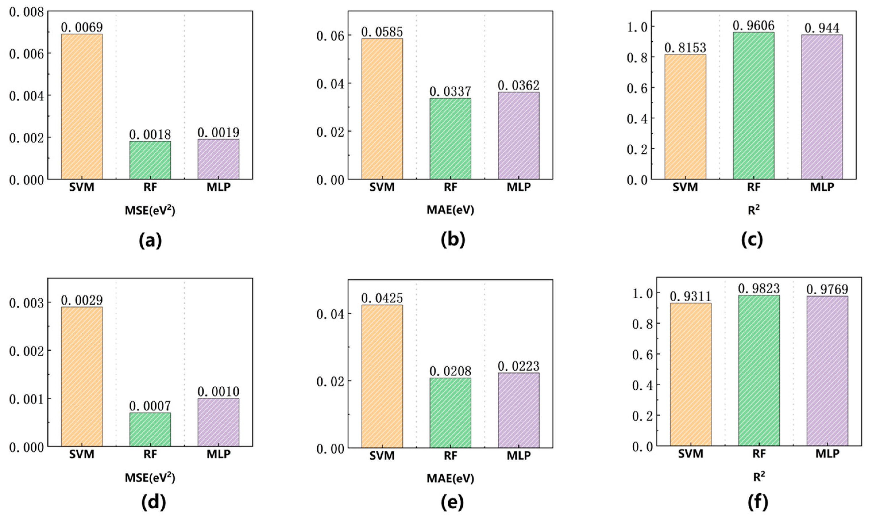
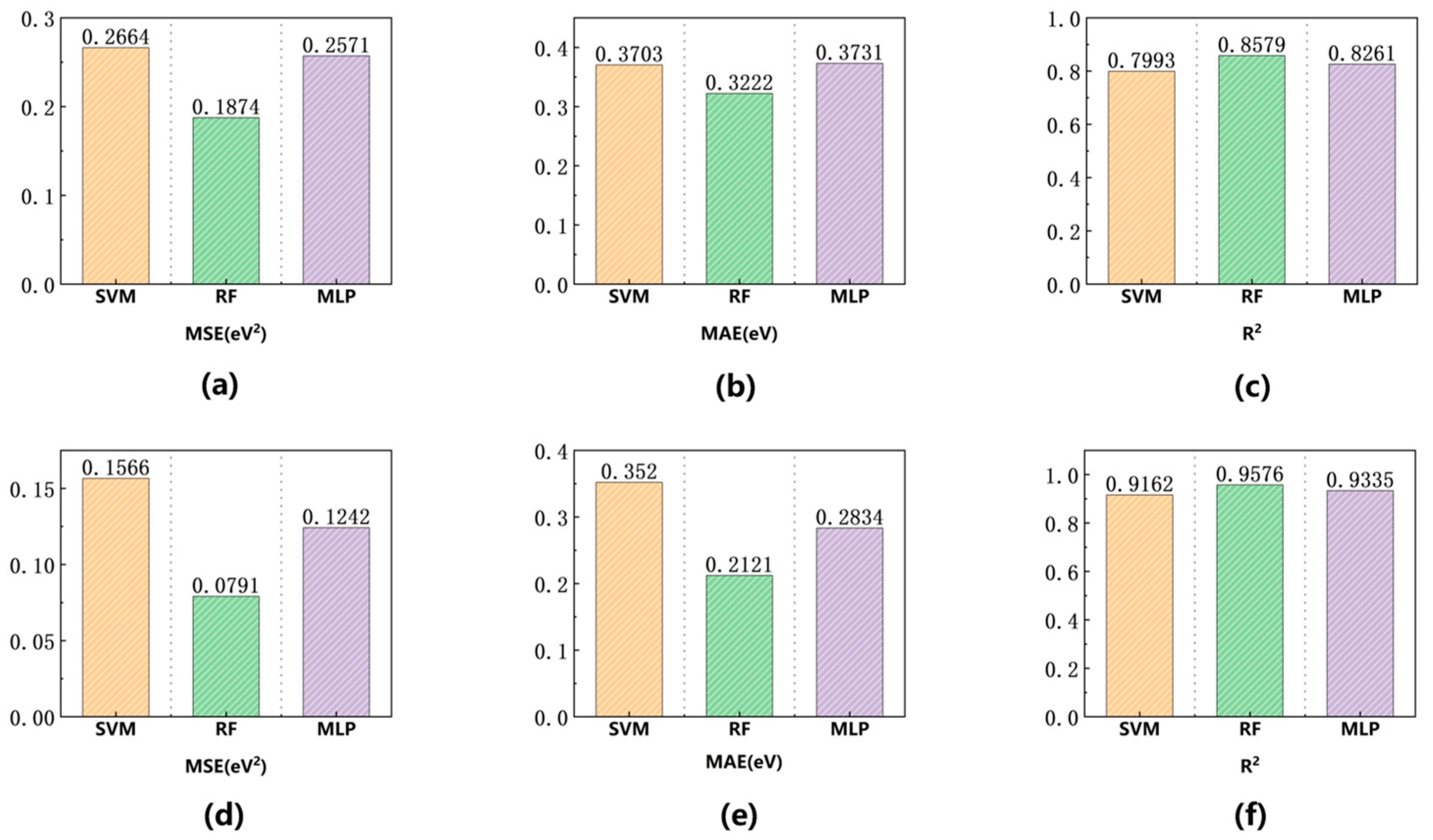
The results of the DFT calculations are quoted as the validation set, and the prediction curves of the three algorithms RF, SVM, and MLP on the bandgap of graphene under the influence of perpendicular external electric field, N doping, and the adsorption rate of H atoms are plotted against the results given in the validation set. Density functional theory calculations serve as the validation set. The figure plots bandgap prediction curves for graphene under the influence of vertical external electric fields, nitrogen doping, and hydrogen atom adsorption rates. These curves were generated by three algorithms: random forest, support vector machine, and multilayer perceptron. The results are compared against the validation set, alongside the mean absolute error (MAE), mean squared error (MSE), and R²; values for the RF, SVM, and MLP models across the test and validation sets. Figure 9a–c and Figure 10a–e and

Table 5. Comparison of graphene bandgap under the influence of vertical electric field in the validation set predicted by SVM model, RF model, MLP model with DFT calculation.

Model	0.0862 (V/nm)	0.335	0.700	1.064	1.428	1.927	2.990
DFT	6.853 (meV)	26.269	67.005	106.980	153.426	202.538	254.315
SVM	9.319	11.154	42.763	81.262	121.990	171.764	218.249
RF	3.748	13.401	49.148	66.949	122.670	158.825	215.992
MLP	1.786	11.477	35.200	75.980	114.983	175.30	216.615

and

Table 6. Comparison of the performance of SVM model, RF model, and MLP model for predicting graphene bandgap under vertical electric field in the validation set.

Model	MSE (eV2)	MAE (eV)	R2	Test Point Error
SVM	674.2302	23.688	0.9605	13.4%
RF	917.4163	26.6645	0.8727	13.6%
MLP	840.5469	27.0266	0.8834	12.7%

present the machine learning model predictions and evaluation results for AB-stacked bilayer graphene under perpendicular external electric fields, respectively. Figure 11a–c and Figure 12a–e and

Table 7. Comparison of N-doped graphene bandgap in the validation set predicted by SVM model, RF model, MLP model with DFT calculation.

Model	2%	4%	6%	8%	10%	12%
DFT	0.14	0.3	0.45	0.54	0.68	0.72
SVM	0.24824	0.25365	0.42019	0.54272	0.70462	0.76299
RF	0.17399	0.30171	0.43926	0.54484	0.70234	0.66835
MLP	0.16117	0.28199	0.44465	0.53021	0.66951	0.66501

and

Table 8. Comparison of the performance of SVM model, RF model, and MLP model for predicting N-doped graphene bandgap in the validation set.

Model	MSE (eV2)	MAE (eV)	R2	Test Point Error
SVM	0.0029	0.0425	0.9311	6%
RF	0.0004	0.0208	0.9823	7.2%
MLP	0.001	0.0223	0.9769	9.6%

, respectively, present the machine learning model predictions and evaluation results for N-doped graphene. Figure 13a–c and Figure 14a–e and

Table 9. Comparison of H-adsorbed graphene bandgap in the validation set predicted by SVM model, RF model, MLP model with DFT calculation.

Model	66.723%	70.716%	74.905%	79.133%	83.166%	87.472%	91.544%	95.811%	100%
DFT	0	0.5571	0.97493	1.26741	1.50418	1.88719	2.44429	3.3078	4.67976
SVM	0.17622	0.39923	1.18484	1.16102	0.95467	1.47579	1.81633	3.75084	4.19398
RF	0.09636	0.53222	0.86319	1.20472	1.06	1.35905	2.96153	3.62186	4.03528
MLP	0.18945	0.55735	0.93019	1.08532	0.87621	1.44179	2.24336	3.02714	4.10075

and

Table 10. Comparison of the performance of SVM model, RF model, and MLP model for predicting H-adsorbed graphene bandgap in the validation set.

Model	MSE (eV2)	MAE (eV)	R2	Test Point Error
SVM	0.1556	0.352	0.9162	10.1%
RF	0.0791	0.2121	0.9576	13.5%
MLP	0.1242	0.2834	0.9335	12%

respectively present the predictions and evaluation results of the machine learning models for H-adsorbed graphene.

3.1. Vertical External Electric Field and Band Gap of Bilayer Graphene

As demonstrated in Figure 9 and Table 5, in conjunction with the findings of Yuanbo Zhang and Tsung-Ta Tang [17], the values of AB stacked bilayer graphene bands at specific external electric field strengths, and the predictions of the three machine learning models are as follows, respectively. According to the findings of the density functional theory (DFT) calculations conducted by Yuanbo Zhang and Tsung-Ta Tang [17], the band gap of the AB stacked bilayer graphene is estimated to be approximately 250 meV at 3 eV/nm. This result is consistent with the band gap of AB stacked bilayer graphene, which is reported to be around 250 meV. In contrast, the results obtained from the random forest (RF) model, support vector machine (SVM) model, and multi-layer perceptron (MLP) model are 215 meV. The 99 eV, 216.61 eV, and 218.24 eV results, with errors of 13.6%, 13.4%, and 12.7%, respectively, indicate the high precision of the three machine learning models.

Secondly, as demonstrated in Figure 10 and Table 6, in the test set, the MSE and MAE values of the SVM model are lower than those of the other two models, and the value of R² is higher than those of the other two models, and it is the smallest error among the three models. This indicates that the SVM model has the best prediction effect in the test set. In the validation set, the SVM model demonstrates the optimal prediction efficacy, thereby substantiating its sufficient generalization capability. Conversely, the MLP model exhibits the poorest prediction performance in the test set. Despite having a smaller MSE value compared to the RF model, the MLP model’s prediction accuracy is inferior when considering the R² and MAE metrics. This outcome is particularly evident in the context of the vertical electric field and the bandgap of bilayered graphene. This phenomenon is further elucidated in Figure 6 where the data points representing the MLP algorithm are dispersed around the y = x line, exhibiting more substantial fluctuations compared to the data points from the other algorithms. A comparison of the SVM model with the other two machine learning models reveals that the predictions of the SVM model are more centrally distributed on a straight line with a slope of 1, indicating less prediction bias. In summary, on the validation set, the SVM model demonstrated the lowest mean squared error (MSE) of 674.2302 meV² and mean absolute error (MAE) of 23.688 meV among the three machine-learning models. Additionally, the R² value of 0.9605 for the SVM model is closest to 1, suggesting that the SVM model exhibits superior performance in predicting the accuracy of the vertical external electric field with respect to the bandgap of AB stacked bilayer graphene.

3.2. N-Doping with Monolayer Graphene Bandgap

In the case of N-doping, the RF model demonstrates notable efficacy in predicting the test set, as evidenced by the strong correlation between the predicted and computed bandgap values in Figure 7a–c and Figure 12a–c. As illustrated in Figure 12a–c, the MSE and MAE of the RF model in the validation set are consistently lower than those of the other two models. The R² value of the RF model reaches 0.9823, indicating an optimal fit.

As demonstrated in Figure 11a–c and Table 7,the disparities between the predictions of the RF, SVM, and MLP models in the validation set are not statistically significant. The band gap values predicted by the RF, SVM, and MLP models are 0.668 eV, 0.763 eV, and 0.651 eV, respectively, when the doping level is 12%. This corresponds to a 7.2% discrepancy when compared to the result of 0.72 eV reported by P Rani and VK Jindal [17]. The differences are 7.2%, 6%, and 9.6%, respectively, which indicates that all three algorithms exhibit excellent prediction performance. A combined analysis of Figure 7 and Figure 13 indicates that the RF algorithm performs optimally.

3.3. H-Atom Adsorption Rate and Band Gap of Monolayer Graphene

As demonstrated in Figure 13 and Figure 14 and Table 9 the rate of hydrogen atom adsorption is contingent upon the band gap of graphane, which, according to the findings of Haili Gao, Lu Wang et al. [23], is approximately 4. The results obtained from the RF, SVM, and MLP models in the present machine learning model are 4.03 eV, 4.19 eV, and 4.1 eV, respectively, with an error of 13.5%, 10.1%, and 12%, respectively. The errors of the prediction results of the three machine learning models are within the acceptable range.

The specific prediction results are illustrated in Figure 14a–e and Table 10, and these results differ from the initial two influences. In the test set and validation set, the values of MAE and MSE of the RF model are lower than those of the other two models, and the value of R² is higher than those of the other two models. This indicates that the RF model shows better results in prediction, while the SVM algorithm has the highest MSE and MAE and the SVM model has the worst performance. This phenomenon is further elucidated in Figure 8a–c, where the points of predicted bandgap values versus calculated bandgap values in the test set of the RF model are observed to be closest to the y = x curve. In contrast, the SVM model exhibits a substantial offset. In the validation set, the results predicted by the RF model are almost exactly correct, and in the first three test points, while the SVM algorithm has shown a large deviation in the first three result points. The RF model demonstrates the most accurate predictions for the rate of H-atom adsorption.

4. Conclusions

This work demonstrates the effective application of machine learning, including support vector machines (SVMs), random forests (RFs), and multi-layer perceptrons (MLPs), to predict the bandgap of graphene under various conditions such as perpendicular electric fields, nitrogen doping, and hydrogen adsorption.

The results show that these models predict the most probable bandgap values at specific concentrations more accurately than absolute values. This suggests the need to consider specific graphene symmetries and structural configurations, rather than treating all possible structures equally, in order to improve prediction accuracy.

There are three primary areas for future improvement. First, the configurations of hydrogen adsorption and nitrogen doping can be further optimized to enhance bandgap tunability. Second, the quality of the dataset generated by Materials Studio can be improved by refining structural parameters and adjusting computational settings. Third, the performance of machine learning models can benefit from more systematic hyperparameter tuning and dataset expansion using MATLAB 2023b, leading to more robust and generalizable predictions.

By combining machine learning with first-principles calculations, this study provides a promising pathway for the rational design of graphene with tunable bandgaps. Furthermore, the methodology established here contributes to the accelerated discovery of two-dimensional materials and supports the development of data-driven approaches for next-generation electronic device design.

References

1. Wallace, P.R. The band theory of graphite. Phys. Rev. 1947, 71, 622–634. [Google Scholar] [CrossRef]
2. Nakada, K.; Fujita, M.; Dresselhaus, G.; Dresselhaus, M.S. Edge state in graphene ribbons: Nanometer size effect and edge shape dependence. Phys. Rev. B 1996, 54, 17954–17961. [Google Scholar] [CrossRef] [PubMed]
3. Novoselov, K.S.; Geim, A.K.; Morozov, S.V.; Jiang, D.; Zhang, Y.; Dubonos, S.V.; Grigorieva, I.V.; Firsov, A.A. Electric field effect in atomically thin carbon films. Science 2004, 306, 666–669. [Google Scholar] [CrossRef] [PubMed]
4. Castro Neto, A.H.; Guinea, F.; Peres, N.M.R.; Novoselov, K.S.; Geim, A.K. The electronic properties of graphene. Rev. Mod. Phys. 2009, 81, 109–162. [Google Scholar] [CrossRef]
5. Schwierz, F. Graphene transistors. Nat. Nanotechnol. 2010, 5, 487–496. [Google Scholar] [CrossRef]
6. Ohta, T.; Bostwick, A.; Seyller, T.; Horn, K.; Rotenberg, E. Controlling the electronic structure of bilayer graphene. Science 2006, 313, 951–954. [Google Scholar] [CrossRef]
7. Icking, E.; Banszerus, L.; Wörtche, F.; Volmer, F.; Schmidt, P.; Steiner, C.; Engels, S.; Hesselmann, J.; Goldsche, M.; Watanabe, K.; et al. Transport spectroscopy of ultraclean tunable band gaps in bilayer graphene. Adv. Electron. Mater. 2022, 8, 2200510. [Google Scholar] [CrossRef]
8. Wang, X.; Ma, C.; Xiao, L.; Xiao, B. Dual-band dynamically tunable absorbers based on graphene and double vanadium dioxide metamaterials. J. Opt. 2024, 53, 596–604. [Google Scholar] [CrossRef]
9. Asgari, S.; Fabritius, T. Multi-purpose graphene-based terahertz metamaterial and its equivalent circuit model. IEEE Access 2025, 13, 56808–56819. [Google Scholar] [CrossRef]
10. Pereira, V.M.; Castro Neto, A.H.; Peres, N.M.R. Strain engineering of graphene’s electronic structure. Phys. Rev. B 2009, 80, 045401. [Google Scholar] [CrossRef]
11. Sofo, J.O.; Chaudhari, A.S.; Barber, G.D. Graphane: A two-dimensional hydrocarbon. Phys. Rev. B 2007, 75, 153401. [Google Scholar] [CrossRef]
12. Withers, F.; Bointon, T.H.; Dubois, M.; Russo, S.; Craciun, M.F. Nanopatterning of Fluorinated Graphene by Electron Beam Irradiation. Nano Lett. 2011, 11, 3912–3916. [Google Scholar] [CrossRef] [PubMed]
13. Zhao, L.; He, R.; Rim, K.T.; Schiros, T.; Kim, K.S.; Zhou, H.; Gutiérrez, C.; Chockalingam, S.P.; Arguello, C.J.; Pálová, L.; et al. Local atomic and electronic structure of doped graphene. Science 2011, 333, 999–1003. [Google Scholar] [CrossRef] [PubMed]
14. Hohenberg, P.; Kohn, W. Inhomogeneous electron gas. Phys. Rev. 1964, 136, B864–B871. [Google Scholar] [CrossRef]
15. Kresse, G.; Furthmüller, J. Efficient iterative schemes for ab initio total-energy calculations using a plane-wave basis set. Phys. Rev. B 1996, 54, 11169–11186. [Google Scholar] [CrossRef]
16. Butler, K.T.; Davies, D.W.; Cartwright, H.; Isayev, O.; Walsh, A. Machine learning for molecular and materials science. Nature 2018, 559, 547–555. [Google Scholar] [CrossRef]
17. Raccuglia, P.; Elbert, K.C.; Adler, P.D.; Falk, C.; Wenny, M.B.; Mollo, A.; Zeller, M.; Friedler, S.A.; Schrier, J.; Norquist, A.J. Machine-learning-assisted materials discovery using failed experiments. Nature 2016, 533, 73–76. [Google Scholar] [CrossRef]
18. Baskin, Y.; Meyer, L. Lattice constants of graphite at low temperatures. Phys. Rev. 1955, 100, 544. [Google Scholar] [CrossRef]
19. Lee, J.K.; Lee, S.C.; Ahn, J.P.; Kim, S.C.; Wilson, J.I.; John, P. The growth of AA graphite on (111) diamond. J. Chem. Phys. 2008, 129, 234709. [Google Scholar] [CrossRef]
20. Rani, P.; Jindal, V.K. Designing band gap of graphene by B and N dopant atoms. RSC Adv. 2013, 3, 802–812. [Google Scholar] [CrossRef]
21. Zhang, Y.; Tang, T.T.; Girit, C.; Hao, Z.; Martin, M.C.; Zettl, A.; Crommie, M.F.; Shen, Y.R.; Wang, F. Direct observation of a widely tunable bandgap in bilayer graphene. Nature 2009, 459, 820–823. [Google Scholar] [CrossRef]
22. Wang, T.; Guo, Q.; Liu, Y.; Sheng, K. A comparative investigation of an AB-and AA-stacked bilayer graphene sheet under an applied electric field: A density functional theory study. Chin. Phys. B 2012, 21, 067301. [Google Scholar] [CrossRef]
23. Gao, H.; Wang, L.; Zhao, J.; Ding, F.; Lu, J. Band gap tuning of hydrogenated graphene: H coverage and configuration dependence. J. Phys. Chem. C 2011, 115, 3236–3242. [Google Scholar] [CrossRef]
Figure 1. A graphene lattice showing the unit cell and primitive lattice vectors.
Physchem 05 00041 g001
Figure 2. The graphene model, constructed by Materials Studio, displays the hexagonal lattice of graphene. The blue and red atoms are represented as C atoms. (a) A top view of a single layer of graphene is shown here. (b) The figure above depicts a top view of an AB stacked bilayer of graphite. In this configuration, the second layer is shifted by one bond length with respect to the first layer along one of the basis vectors of the honeycomb lattice.
Physchem 05 00041 g002
Figure 3. (ac) represent three random structures of graphene with a 5.2% N doping rate, respectively, with random N doping positions. The crystal structure was constructed using Materials Studio, where the red atoms are N atoms and the blue atoms are C atoms.
Physchem 05 00041 g003
Figure 4. Chair conformation of partially hydrogenated graphene with 39% hydrogen absorption, model constructed by Materials studio, can be observed as a hexagonal lattice of graphene sp3-hybridized, where the red atoms are the H atoms and the blue atoms are the C atoms: (a) top view (b) side view.
Physchem 05 00041 g004
Figure 5. (ac) illustrate the training set data distributions for graphene with an external electric field, N-doped graphene, and H-adsorbed graphene, respectively, when the number of bins is 10. (df) illustrate the data distributions when the number of bins is 12. The vertical axis of the graph represents the number of data samples in each interval.
Physchem 05 00041 g005
Figure 6. Vertical external electric field and graphene band gap prediction results on the test set. In the three plots, the blue curves all indicate the y = x function curves, and the values predicted by the RF model, the SVM model, and the MLP model are labeled in yellow, pink, and red: (a) RF model (b) SVM model (c) MLP model.
Physchem 05 00041 g006
Figure 7. N-doping and graphene bandgap prediction results on the test set. In all three plots, the blue curves indicate the y = x function curves, and the values predicted by the RF model, the SVM model, and the MLP model are labeled in yellow, pink, and red: (a) RF model (b) SVM model (c) MLP model.
Physchem 05 00041 g007
Figure 8. H adsorption rate and graphene band gap prediction results on the test set. In all three plots, the blue curves indicate the y = x function curves, and the values predicted by the RF model, the SVM model, and the MLP model are labeled in yellow, pink, and red: (a) RF model (b) SVM model (c) MLP model.
Physchem 05 00041 g008
Figure 9. Evaluation of AB stacked bilayer graphene bandgap validation set under the influence of vertical external electric field, the red folded line is the result of DFT calculation in the validation set, and the prediction results of RF, SVM, and MLP models are marked by blue, purple, and yellow curves: (a) RF model (b) SVM model (c) MLP model.
Physchem 05 00041 g009
Figure 10. Vertical external electric field with AB stacked bilayer graphene machine learning model evaluation, metrics for SVM model, RF model, and MLP model are shown as yellow, green, and purple bars: (a) Test set MSE, (b) Test set MAE, (c) Test set R2, (d) Validation set MSE, (e) Validation set MAE, (f) Validation set R2.
Physchem 05 00041 g010
Figure 11. Evaluation of N-doped graphene bandgap in the validation set, the red folded line is the result of DFT calculation in the validation set, and the prediction results of RF, SVM, and MLP models are marked by blue, purple, and yellow curves: (a) RF model, (b) SVM model, (c) MLP model.
Physchem 05 00041 g011
Figure 12. N-doped graphene machine learning model evaluation, metrics for SVM model, RF model, and MLP model are shown as yellow, green, and purple bars: (a) test set MSE, (b) test set MAE, (c) test set R2, (d) validation set MSE, (e) validation set MAE, (f) validation set R2.
Physchem 05 00041 g012
Figure 13. Evaluation of H-adsorbed graphene bandgap in the validation set, the red folded line is the result of DFT calculation in the validation set, and the prediction results of RF, SVM, and MLP models are marked by blue, purple, and yellow curves: (a) RF model, (b) SVM model, (c) MLP model.
Physchem 05 00041 g013
Figure 14. H adsorption graphene machine learning model evaluation, metrics for SVM model, RF model, and MLP model are shown as yellow, green, and purple bars: (a) test set MSE, (b) test set MAE, (c) test set R2 (d) validation set MSE, (e) validation set MAE, (f) validation set R2.
Physchem 05 00041 g014