Enhancing Predictive Accuracy Under Data Scarcity: Modeling Molecular Interactions to Describe Sealing Material Compatibility with Bio-Hybrid Fuels

Abstract

Bio-hybrid fuels, chemically derived from sustainable raw materials and green energies, offer significant potential to reduce carbon dioxide emissions in the transport sector. However, when these fuels are used as drop-in replacements in internal combustion engines, material compatibility with common sealing materials is not always given. Within the cluster of excellence, “The Fuel Science Center (FSC)” at RWTH Aachen, experimental immersion tests were conducted on a limited set of fuel and sealing material combinations. Given the extensive range of possible fuel and sealing combinations, a data-based machine learning prediction framework was developed and validated to pre-select promising fuel candidates. Due to the limited number of samples, preliminary results indicate a need to expand the database. Since experimental investigations are time-consuming and costly, this work explores faster physics-motivated data generation approaches by modeling molecular interactions between fuel and sealing materials. Two modeling scales are employed. One calculates the intermolecular distance using density functional theory. The other uses Hansen solubility parameters, representing an abstract modeling of intermolecular forces. Both approaches are compared, and their limitations are assessed. Including the generated data in the prediction framework improves its accuracy.

1. Introduction

Given the need to explore alternative propulsion systems in the transportation sector, liquid bio-hybrid fuels emerge as a promising energy carrier. Bio-hybrid fuels summarize multiple fuels that combine carbon sources, such as renewable feedstock or waste, with external energy inputs. The production process incorporates renewable energy or biological processes to elevate the energy state of the base product, enabling the synthesis of fuels with a high energy density. Complementing battery-electric, hydrogen, and ammonia-powered systems, the fuels’ high energy density makes them especially suitable for difficult-to-electrify applications, such as aircrafts and heavy-duty machinery.

Within the Cluster of Excellence “The Fuel Science Center (FSC)” at RWTH Aachen University, these fuels are studied holistically, focusing on developing methods to identify optimal fuel candidates that balance environmental, economic, and technical requirements. This is achieved through an interdisciplinary fuel design process, addressing fuel properties so that they comply with current standards and regulations. This includes engine (combustion)-relevant properties such as research octane number (RON) [1,2], ignition delay time (IDT) [3,4], or catalytic activity in the exhaust system, fluid mechanical and rheological properties such as density, viscosity, and surface tension [5,6], as well as toxicological assessments [2].

The full potential of these fuels can only be realized when they are used in existing combustion systems as “drop-in” fuels, requiring no significant modifications to the current infrastructure. However, this requires material compatibility with all system components, mainly static and dynamic seals. Previous studies and immersion tests have shown that especially many bio-hybrid fuels are incompatible with conventional elastomer sealing materials. These interactions can cause significant swelling, with elastomer volume increasing by over 200%, leading to immediate failure in technical applications. Alongside swelling, additional wear mechanisms, such as changes in hardness and chemical reactions, have also been observed. With these investigations, suitable sealing material for existing fuels can be identified, or conversely, fuels or fuel blends can be optimized for improved material compatibility [5,7,8].

However, the field of potential fuel candidates, blends, and sealing material combinations is vast, making a comprehensive investigation impractical. Additionally, immersion tests are manually intensive, time-consuming, and costly, highlighting the need for a targeted experimental design to select combinations for further strategic study. To address this, a supervised machine learning regression approach has been developed to predict elastomer property changes for specific fuel and seal combinations after immersion. A pairing is considered valid if the predicted property changes in the sealing material fall within predefined value ranges. These ranges are derived from current fuel standards, observations with conventional fuels, and plausible technical limitations, such as a maximum allowable volume increase of, for example, $50\%$. Combinations with values that deviate significantly from this range are excluded from further consideration, thereby narrowing down the field of possible combinations [9].

An initial application of the framework highlights the need for optimization, as model evaluation reveals generally low training and testing scores. This is primarily due to the limited data samples [9]. In addition to ongoing experimental data generation and model refinements, this study proposes alternative, faster approaches for generating data by modeling the interactions between the fuel and sealing material. The assessment of the quality of such simulated data for usage in a supervised machine learning model in the context of predicting material compatibility is the task of this paper.

After an introduction to the general ML process, examples showcase its application in fluid power systems and the fuel design process. Subsequently, two methods used in this work to model the interaction between fuel and elastomer are introduced: one approach models interactions at the quantum-mechanical level, known as density functional theory (DFT), while the other provides a more generalized, abstract representation, referred to as the Hansen solubility parameters (HSPs) [10].

Section 2 introduces the process of the experimental data generation and details the architecture of the prediction framework. Additionally, the methodologies for synthetic data generation, including both DFT-based and HSP-based approaches, are presented. Results are presented in Section 3, which is structured in three parts. First, the outcomes of the data generation process are presented, detailing the characteristics and reliability of the synthetic data. Second, the baseline results, obtained using only experimental data within the prediction framework, are analyzed to establish a reference for comparison. Finally, the impact of incorporating synthetic data is evaluated by comparing the prediction performance between the baseline and extended database cases. The results of both cases are analyzed in Section 4, focusing on the effects of dataset expansion on model performance and identifying key areas for future refinement. The overall structure of this work is visually represented in Figure 1.

1.1. Machine Learning Application

Machine learning is a branch of artificial intelligence that enables computers to learn patterns from data and make decisions without explicit programming. The general process involves data collection and pre-processing, model selection, training to extract underlying patterns, and evaluation to refine predictions. This methodology has been successfully applied across a range of domains, including fluid power, physical and chemical system modeling, and material science.

Recent advancements in physics-informed machine learning have demonstrated significant success in tribological investigations, where ML models are integrated with physical laws to enhance prediction accuracy and interpretability [11,12,13,14,15,16]. In the field of fluid power, ML has been employed for fault detection [17] and condition monitoring of hydraulic systems [18,19], illustrating its potential to improve system reliability and performance by identifying anomalies and predicting failures. Historically, the prediction of material compatibility—particularly in hydraulic systems—has relied on group contribution methods to estimate Hansen solubility parameters (HSPs) [20].

In the context of fuel design, ML techniques have been leveraged for uncertainty quantification [21] and for predicting key properties such as fuel ignition quality using graph neural networks [1]. Additional investigations have focused on the material compatibility of bio-hybrid fuels and elastomers using HSP-based methods [7], and ML frameworks have been developed for the evaluation of drop-in aviation fuels [22].

1.2. Interaction Simulation HSPs and DFT

This work explores two methods to model intermolecular interactions between fuels and sealing materials. The extent of intermolecular interaction between the fuel and elastomer is a crucial point to consider when evaluating material compatibility. Failure of the sealing material is a result of swelling of the elastomer, which in turn is a result of the sealing elastomer interacting with the fuel molecules on a molecular level. A common approach to assess material compatibility involves describing the interactions using three numerical parameters known as Hansen solubility parameters. Another approach involves quantum-mechanical analysis of molecular interactions using density functional theory (DFT). This method iteratively calculates the equilibrium state between two molecules and determines the parameters characterizing this state. In the subsequent sections, both approaches are introduced.

• HSP

The concept of Hansen solubility parameters (HSPs) is commonly used to select suitable solvents for a given solute. The principle of “like dissolves like” predicts solubility when the intermolecular forces of the solvent and solute are similar in type and strength. An initial approach to predict the solubility of two substances was proposed by Hildebrand based on the eponymous Hildebrand parameter ${\delta }_T$. This parameter is defined as the square root of the cohesive energy density of a substance, where V is the molar volume of the pure substance, and E is its energy of vaporization [23].

$${\delta }_T={(E/V)}^{1/2}$$

(1)

However, this single parameter proved to be insufficient to fully represent the complex interactions between different molecules. Therefore, Hansen expanded Hildebrand’s approach and further divided the binding energy into the proportions caused by dispersive forces $E_D$ by polar forces $E_P$, and by forces caused by hydrogen bonds $E_H$ [10].

$$E=E_D+E_P+E_H$$

(2)

Again, dividing each component of the binding energy by the molar volume yields the three squared Hansen solubility parameters (HSPs), ${\delta }_D$, ${\delta }_P$, and ${\delta }_H$, which in total are equal to the Hildebrand solubility parameter.

$${\delta }_T^2={\delta }_D^2+{\delta }_P^2+{\delta }_H^2$$

(3)

Each substance (molecule) can be located in the three-dimensional HSP space with these three parameters. The Euclidean distance $Ra$ between the locations of two molecules in this space indicates the similarity of these molecules. Smaller distances suggest greater solubility potential between the substances. The dispersive parameter is weighted by a factor of four, which was determined empirically.

$$Ra=\sqrt{4({\delta }_{D2}-{\delta }_{D1})+({\delta }_{P2}-{\delta }_{P1})+({\delta }_{H2}-{\delta }_{H1})}$$

(4)

Generally, HSPs are obtained via experimental investigations, but HSP values are available for many pure substances in the literature. Furthermore, HSPs can be calculated using the group contribution method or QSPR. However, since this work initially focuses only on pure and common substances, values from the literature [10] are utilized in the following to predict numerical volume change values for data generation.

• DFT

Examining the system on a molecular level enables an analysis of the elastomer–fuel interaction. To allow for a quantitative interpretation of this interaction, a minimum accuracy needs to be obtained using the chosen method. Due to the inherent lack of electron correlation and thus limited accuracy in Hartree–Fock theory, as well as the increasing cost of calculation in terms of CPU hours for post-Hartree–Fock methods, DFT offers a good trade-off between accuracy and cost for electronic structure calculation of organic molecules.

The electronic properties of a chemical system are related to the system’s electronic wave function. For one-electron systems, the wavefunction can be determined via an analytical solution of the Schrödiger equation. However, this cannot be done for systems involving more than one electron. This is where density functional theory (DFT) comes into play for electronic structure calculations.

The central variable in DFT is the electron density $\rho$, which relates to the probability of finding any electron at place $\mathbf{r}$. This relationship is shown in Equation (5) using the formalism of the Born rule that states that the probability of electron residency in a specific place is proportional to the square of the amplitude of the wave function $\mathsf{\Psi }$ [24].

$$\rho \left(\mathbf{r}\right)=n\int \mathsf{\Psi }{\left(\mathbf{x},{\mathbf{x}}_2,\dots ,{\mathbf{x}}_n\right)}^{*}\mathsf{\Psi }\left(\mathbf{x},{\mathbf{x}}_2,\dots ,{\mathbf{x}}_n\right)\mathrm{d}{m}_s\mathrm{d}{\mathbf{x}}_2\dots \mathrm{d}{\mathbf{x}}_n$$

(5)

The mathematical foundation of DFT lies in the Hohenberg–Kohn thorem (see Equation (6)), which postulates the existence of a functional of the density $F\left[\rho \right(\mathbf{r}\left)\right]$ that expresses the correct ground state energy $E_0$ of the system and thus allows for the description of such systems using the electron density [25].

$$E_0=F\left[{\rho }_0\left(\mathbf{r}\right)\right]$$

(6)

Kohn and Sham made this approach computationally accessible by implementing orbitals of a comparison system of non-interacting fermions (Kohn–Sham orbitals) into the mathematical treatment (Kohn–Sham DFT) [26]. However, a description of the underlying universal exchange correlation functional has not been successful. But, various functionals approximate the relationship between electron density and exchange correlation energy for different applications to different extents. These functionals are classified into categories and arranged on Jacob’s ladder [27]. Here, the user must make a trade-off between increasing the complexity and accuracy of the functional on one side and increasing computational cost on the other.

In the past, DFT was used in various studies to research intermolecular interactions. Examples include the work of Miranda-Quintana et al. [28], which used minimum-interaction energies from DFT to predict the reactive behavior of a pair of reagents. The so-called “conceptual DFT” has been proven to explain general chemical concepts like the HSAB principle [29], emphasizing the importance of this theory for interpreting intermolecular interactions. DFT has also contributed to the development of various descriptors regarding reactivity; for example, the prediction of site reactivity in substituted phenyl molecules [30], further explaining chemical interactions between molecules.

With the development of computational methods that account for long-range interactions, the prediction of intermolecular interaction energies becomes more accurate [31]. In the context of researching polymer–solvent intermolecular interactions, DFT was used by Yamada et al. [32] to quantify NBR–solvent interactions, leading to theoretical results in good agreement with experimental results. Similarly, through DFT, Wu et al. investigated intermolecular interactions between a polyacrylonitrile polymer and different solvent molecules [33].

2. Materials and Methods

This section introduces the methods and procedures for data generation, both empirical and simulation-based, and the implementation of the prediction framework. To date, only experimental data have been used to train and evaluate the prediction framework. This study investigates the contribution of simulated data to the accuracy of prediction.

2.1. Experimental Data Generation

Central to the investigation of elastomer compatibility are immersion tests conducted following ISO 1817 [34]. Standard reference elastomer NBR (SRE-NBR 28/SX), according to DIN ISO 13226 [35], was immersed in different bio-hybrid fuels and pure fuel components for 28 days. Specimens measuring 25 × 25 × 2 mm³ were fully submerged in sufficient fuel throughout the test duration. The use of SRE, with its known composition and absence of additives, enables comparison of results with the literature and previous studies while isolating the influence of individual fuel properties and constituents.

During the testing period, changes in elastomer mass, volume, and hardness were evaluated following DIN 53521 [36] at defined time intervals. Of particular importance in assessing elastomer compatibility are the changes in specimen properties, specifically the volume change $\mathsf{\Delta }V$ and hardness change $\mathsf{\Delta }H$ at the final interval (V and H) relative to their initial states ($V_0$ and $H_0$) (see Equation (7)). These results are shown in Figure 2. For a detailed description of the measurement principles, see Hofmeister et al. [5,8]. At this stage, only volume change data are considered for further use throughout this study.

$$\mathsf{\Delta }V={\displaystyle \frac{V-V_0}{V_0}}·100,\mathsf{\Delta }H={\displaystyle \frac{H-H_0}{H_0}}·100$$

(7)

2.2. Prediction Framework

Central to this study is the ML prediction framework developed and initially validated in [9]. This section introduces the structure of this framework.

A supervised learning (SL) regression approach was chosen to predict the property changes of elastomers. A numerical value was computed using a dataset containing input features and corresponding target variables (labels). In SL, a model is trained to predict the actual output, called a label, based on given inputs. In this case, the input parameters for the ML models were combined in a molecular fingerprint, which was generated for each fuel candidate using the open-source cheminformatics Python library RDKit [37] and Mordred [38]. Molecular fingerprints are digital representations of chemical structures, capturing essential information such as molecular size, shape, and chemical properties in a one-dimensional vector. Here, molecular fingerprints represent, among others, key fuel properties related to molecular size and polarity, which have been identified as influencing the volume and hardness changes of elastomer specimens when immersed in different fuels. The labels are the measured volume changes obtained from previous immersion tests. This represents a single-output regression problem, where linear and nonlinear models can be used to predict the target value. Rather than selecting one single model, the framework can account for multiple models subsequently.

The framework is implemented in Python 3.10, allowing library extensions that access mathematical and machine learning toolboxes. This study’s library list is shown in

Table 1. List of utilized libraries.

Library	Use Case
Pandas [40]	Data manipulation and analysis Handling structured data (e.g., tables, spreadsheets)
Numpy [41]	Numerical computing and array processing Support for multi-dimensional arrays and matrices
Matplotlib  [42]	Data visualization and plotting
Scikit-learn [39]	Machine learning and statistical modeling Tools for regression and dimensionality reduction Preprocessing and evaluation of models
PubChemPy [43]	Interfacing with the PubChem database for chemical information Fetching compound details, names, and SMILES
RDKit [37]	Cheminformatics and molecular modeling Generating molecular descriptors and 3D conformers Substructure searching and visualization of molecular structures
Mordred [38]	Calculating molecular descriptors for cheminformatics Supports a wide range of descriptor types (e.g., physical, chemical, topological)

. Among the tools provided by scikit-learn [39], the framework utilizes four built-in regression models: linear regression, lasso regression, multi-layer perceptron (MLP) regression, and decision tree regression.

The dataset, stored in an Excel file, linked each fuel or pure fluid’s CAS number to its corresponding SRE-NBR volume changes. During data input to the framework, the canonical SMILES representation was generated for each CAS number using PubChemPy [43]. A 3D molecular model was then constructed using RDKit [37], and all molecular descriptors were calculated using Mordred [38]. This way, 1826 numerical features were obtained for each data sample. Their correlation to the target value (volume change) was first calculated to consider only the most influential features. Then, they were sorted in descending order based on their correlation score. Subsequently, features with a correlation score below an absolute threshold of $0.33$ were removed. In doing this, the number of features was reduced by a factor of around 30.

Next, a common drawback inherent to data-driven algorithms was addressed by applying feature scaling to the input data. This normalizes the features in a typical band, resolving the issue of different units and magnitudes in the input data. Scaling was performed by applying a standard scaler, which normalizes each feature by subtracting its mean and dividing it by its standard deviation. This transformation ensures each feature has a mean of 0 and a standard deviation of 1 [9]. Another drawback, especially in the framework’s development phase, is the high dimensionality of features alongside a limited amount of data samples. Hence, a principal component analysis (PCA) was performed to reduce dimensionality by transforming the original features into a new set of orthogonal, uncorrelated variables. The number of principal components was selected based on the available data samples, with approximately 10 data samples corresponding to each input feature. Lastly, it was ensured that the model architecture was optimally adapted the given data. This adjustment ensures optimal performance. However, the field of possible model architectures is almost infinite. Therefore, automated/heuristic/model-based algorithms such as halving grid search CV were implemented in the framework.

Due to the small dataset (n = 49), statistical uncertainties arose, which were addressed within the framework using k-fold cross-validation. The data were divided into five non-overlapping subsets. For each subset, hyperparameter tuning was performed. The best model was then evaluated using $R^2$ metrics. This process was repeated for all folds, and the average scores were calculated to facilitate model comparison.

2.3. Simulative Data Generation

The impact of incorporating physics-related synthetic data on the accuracy of the prediction framework is central to this study. This section, therefore, introduces the process for generating data samples without additional experiments. Fundamental to this method are the previously presented approaches, HSP and DFT, which characterize the interactions between fuel and elastomer with numerical values. These values predict the volume increase for fuel candidates and pure substances that have not been experimentally tested. The newly generated data samples were then integrated into the prediction framework to enhance its capabilities.

The process was divided into the following steps. First, the corresponding values were either retrieved from the literature, as in the case of HSP, or calculated using the DFT approach. This was done for all previously tested fuel candidates for which the volume increase was known based on experiments (see Table 3). In a subsequent step, the correlation between these values and the volume increase was learned by a supervised learning regression model similar to the one presented in the prediction framework above. Instead of molecular descriptors, the values resulting from HSP and DFT served as input features and described each substance. Lastly, the trained model was applied to previously unseen fuel candidates. A few fuel candidates validated the prediction accuracy during data generation.

In the following, the HSP and DFT values considered are introduced. The three HSPs, ${\delta }_D$, ${\delta }_P$, and ${\delta }_H$, and the molar volume $V_M$ of one substance are considered as values for the HSP approach. These values are available from the literature. Next, the DFT computational process is described.

Figure 3 shows the computational process of simulating NBR/fuel molecule intermolecular distance d and binding enthalpies $\mathsf{\Delta }E$ using density functional theory.

Different fuel species were considered in this study. These molecules were selected based on the availability of experimental data from swelling tests at the FSC. For the elastomer species, cis-butadiene-acrylonitrile-trans-butadiene was used as the model polymer unit according to [32] as it includes the different functional groups present in NBR.

After building the single molecules in Avogadro [44], quantum mechanical geometry optimization was performed using ORCA 5.0 [45]. The underlying level of theory is presented later in this chapter. Then, Mulliken population analysis was performed to determine the charge distribution in the respective molecules, i.e., finding the most positively (and negatively) charged atoms in the molecules based on the assumption that these are the main points of interaction [32]. Based on this analysis, a spatial orientation of an interacting fuel molecule–NBR complex was approximated, and geometry optimization of this complex was performed with the same level of theory. Differences in the sum of the enthalpy of the single molecules and the fuel molecule–NBR complex were considered to determine the binding enthalpy $\mathsf{\Delta }E$. The intermolecular distance d can be abstracted from the optimized geometry by measuring the the shortest distance between the nitrogen atom in the model NBR molecule and the most positively charged hydrogen atom in the fuel molecule.

All geometry optimizations were performed using the Karlsruhe triple-zeta basis set def2-TZVPP [46] together with the meta-GGA exchange correlation functional r2Scan [47]. D3BJ dispersion correction [48] was used to account for medium-range correlation, thus providing higher accuracy. The auxiliary basis set def2/J was used to speed up the calculation through the resolution of the identity Coulomb integral approximation [49]. The underlying level of theory for the geometry optimizations is summarized in

Table 2. Level of theory used for the DFT geometry optimization.

Functional	Basis Set	Coulomb Approx.	Dispersion Corr.
r2SCAN	def2-TZVPP	def2/J	D3BJ

.

3. Results

In this chapter, the results of this study are presented. The first section focuses on the data generation process, detailing the outcomes of the simulations and their reliability. The second section evaluates the predictive framework using experimental data, establishing a baseline performance score. Finally, the third section explores the impact of integrating simulated data with experimental data, assessing how this combined approach influences the predictive accuracy of the framework.

3.1. Simulated Data Results

Table 3. Substance data with DFT and HSP features and corresponding target values.

Name	CAS	DFT		HSP				Target
		$\mathit{d}$	$\mathbf{\Delta }\mathit{E}$	${\mathit{\delta }}_{\mathit{D}}$	${\mathit{\delta }}_{\mathit{P}}$	${\mathit{\delta }}_{\mathit{H}}$	${\mathit{V}}_{\mathit{M}}$	$\mathbf{\Delta }\mathit{V}$
		[Å]	$\mathbf{\left[}{\mathbf{E}}_{\mathbf{h}}\mathbf{\right]}$	$\mathbf{\left[}{\mathbf{MPa}}^{\mathbf{1}\mathbf{/}\mathbf{2}}\mathbf{\right]}$	$\mathbf{\left[}{\mathbf{MPa}}^{\mathbf{1}\mathbf{/}\mathbf{2}}\mathbf{\right]}$	$\mathbf{\left[}{\mathbf{MPa}}^{\mathbf{1}/\mathbf{2}}\mathbf{\right]}$	$\mathbf{\left[}{\displaystyle \frac{{\mathbf{cm}}^{\mathbf{3}}}{\mathbf{mol}}}\mathbf{\right]}$	[%]
1,3-Dioxolane	646-06-0	2.593	−0.0099	18.1	6.6	9.3	69.9	199.20
Di-n-butyl ether	142-96-1	3.194	−0.0086	15.2	3.4	4.2	170.3	28.30
Isopropanol	67-63-0	2.046	−0.0120	15.8	6.1	16.4	76.8	15.20
Dimethoxyethane	109-87-5	2.684	−0.0105	15	1.8	8.6	169.4	102.10
Ethanol	64-17-5	2.094	−0.0103	15.8	8.8	19.4	58.5	15.45
Methanol	67-56-1	2.067	−0.0098	15.1	12.3	22.3	40.7	9.68
Cyclopentane	287-92-3	2.923	−0.0021	16.4	0	1.8	94.9	3.81
Cyclopentanone	120-92-3	2.849	−0.0065	17.9	11.9	5.2	89.1	197.14
Butyl alcohol	71-36-3	1.989	−0.0134	15.8	5.7	14.5	92	148.73
Acetophenone	98-86-2	2.841	−0.0111	19.6	8.6	3.7	117.4	182.43
Propylene carbonate	108-32-7	3.03	−0.0119	20	18	4.1	85.2	40.60
E-caprolactone	502-44-3	2.644	−0.0087	19.7	15	7.4	110.8	145.15
Bromobenzene	108-86-1	2.568	−0.0098	20.5	5.5	4.1	105.3	182.40
2-Methylfuran	534-22-5	2.803	−0.0076	17.3	2.8	7.4	89.7	102.47
Heptane	142-82-5	5.344	−0.0063	15.3	0	0	147.4	10.52
n-Butanal	123-72-8	3.592	−0.0066	15.6	10.1	6.2	90.5	61.61
n-Pentanal	110-62-3	2.74	−0.0077	15.7	9.4	5.8	106.4	40.90
Acetone	67-64-1	2.893	−0.0059	15.5	10.4	7	74	89.60
2-Butanone	78-93-3	4.171	−0.0117	16	9	5.1	90.2	117.99
Methyl isobutyl ketone	108-10-1	3.819	−0.0071	15.3	6.1	4.1	125.8	108.30
Isopropyl methyl ketone	563-80-4	2.607	−0.0097	7.2	3	4	107	105.90
Diisopropyl ketone	565-80-0	3.273	−0.0111	-	-	-	-	136.40
1-Decanol	112-30-1	1.985	−0.0124	16	4.7	10	191.8	13.64
Benzyl alcohol	100-51-6	1.977	0.1218	18.4	6.3	13.7	103.6	134.70
Tert-butanol	75-65-0	2.059	−0.0123	15.2	5.1	14.7	95.8	24.74
2-Methoxyethanol	109-86-4	2.024	−0.0136	16	8.2	15	79.3	40.79
2-Chlorophenol	95-57-8	1.965	−0.0186	20.3	5.5	13.9	102.3	243.04
Cyclohexanol	108-93-0	2.359	−0.0111	17.4	4.1	13.5	106	34.34
1-Hexanol	111-27-3	-	-	15.9	5.8	12.5	124.9	20.03
1-Octanol	111-87-5	-	-	16	5	11.9	157.7	17.70
1-Octene	111-66-0	-	-	15.3	1	2.4	158	13.26
2,2,4-Trimethylpentane	540-84-1	-	-	14.1	0	0	166.1	10.53
2-Methyl tetrahydrofuran	96-47-9	-	-	16.9	5	4.3	100.2	128.02
2-Octanol	123-96-6	-	-	16.1	4.9	11	159.1	14.96
Benzene	71-43-2	-	-	18.4	0	2	89.4	124.33
Cyclohexanone	108-94-1	-	-	17.8	6.3	5.1	104	178.20
Decane	124-18-5	-	-	15.7	0	0	195.9	7.92
Dodecane	112-40-3	-	-	16	0	0	228.6	8.30
Dodecanol	112-53-8	-	-	16	4	9.3	224.5	12.11
Ethyl acetate	141-78-6	-	-	15.8	5.3	7.2	98.5	122.60
Ethylbenzene	100-41-4	-	-	17.8	0.6	1.4	123.1	113.29
Hexadecane	544-76-3	-	-	16.3	0	0	294.1	5.32
Hexanal	66-25-1	-	-	15.8	8.5	5.4	120.2	23.49
Octane	111-65-9	-	-	15.5	0	0	163.5	11.10
Toluene	108-88-3	-	-	18	1.4	2	106.8	110.60
Cyclohexane	110-82-7	-	-	16.8	0	0.2	108.7	29.84
Diethyl ketone	96-22-0	-	-	15.8	7.6	4.7	106.4	116.56
2-Octanone	111-13-7	-	-	7.4000	3.5000	1.9	157.3	0.823697

lists all substances experimentally investigated within the FSC and their corresponding HSP and DFT values used as input features. DFT data were calculated for 28 substances, while HSP values were obtained from the literature for 47 substances. The missing DFT results are due to non-converging calculations caused by complex molecular structures. Furthermore, the elastomer volume changes (target) for all of the investigated substances are listed in Table 3.

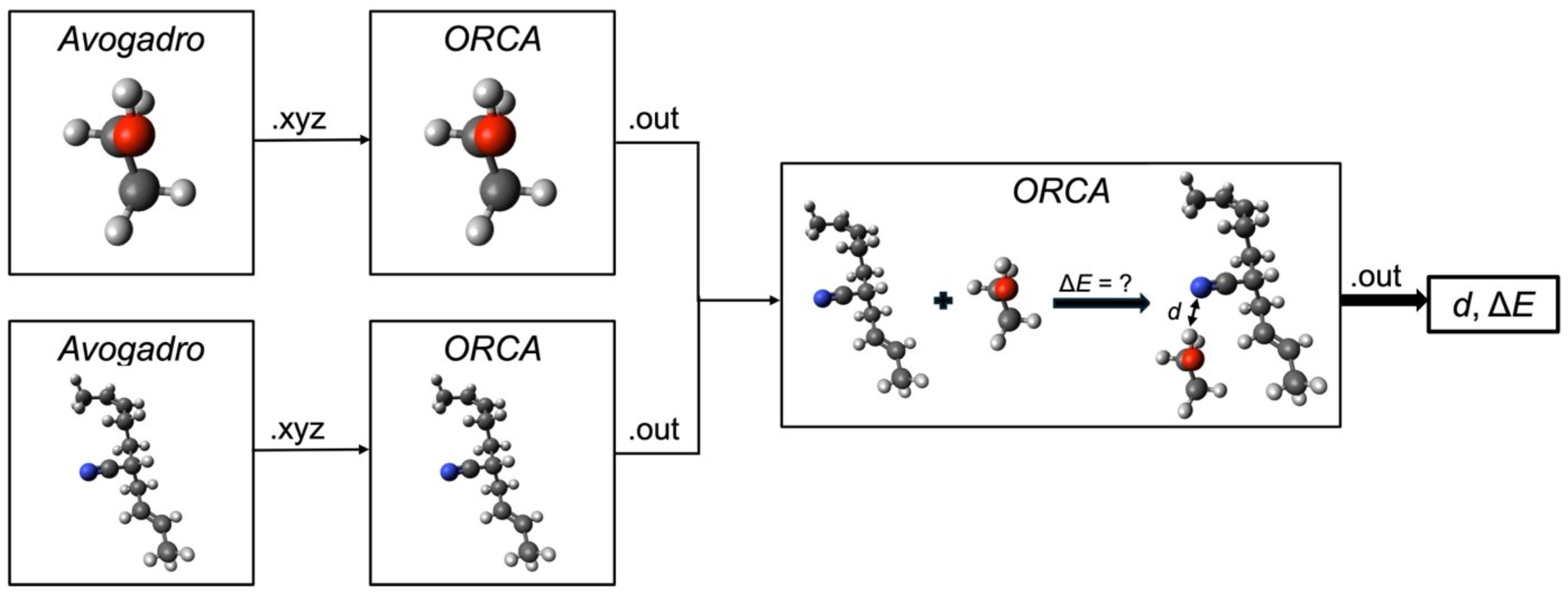
An initial investigation into the suitability of the gathered values for the data generation process revealed an unfavorable case for the DFT approach. Using the Pearson correlation coefficient to assess the strength of the correlation between individual values and the target variable, volume change, it becomes evident that no significant correlation exists for the DFT values. The calculated intermolecular distance d and binding enthalpy $\mathsf{\Delta }E$ yielded correlation scores of $-0.0732$ and $0.0888$, respectively. In contrast, the correlation scores for the HSPs were equal or greater than $0.2637$ for all parameters except ${\delta }_H$ (see

Table 4. Pearson correlation of DFT and HSP values with change in volume.

	DFT $\mathit{n}=28$		HSP $\mathit{n}=46$
	$\mathit{d}$	$\mathbf{\Delta }\mathit{E}$	${\mathit{\delta }}_{\mathit{D}}$	${\mathit{\delta }}_{\mathit{P}}$	${\mathit{\delta }}_{\mathit{H}}$	${\mathit{V}}_{\mathit{M}}$
Pearson correlation r	$-0.0732$	$0.0888$	$0.3690$	$0.2637$	$-0.0030$	$-0.4026$
Only for alcohol $n=7$	$-0.6883$	$0.5791$

). However, closer examination of the DFT values highlights the limited usability of the DFT approach, at least for the functional group of alcohols. Among the 28 substances for which DFT values were calculated, 7 belonged to the functional group of alcohols. When considering only these substances, the correlation with the target values was significantly higher, suggesting that the DFT approach may still hold potential for specific functional groups (see Table 4). However, since the approach in this study should apply to substances across all functional groups, the overall low correlation—alongside the limited number of DFT data samples—makes the DFT approach less suitable for further use in the prediction process. Hence, only HSPs predict the volume change for previously untested substances.

The poor performance of the DFT results could be due to the inherent drawbacks of DFT. While the theory of DFT is exact, the exchange-correlation functional is not known and hence all DFT functionals are approximations. Also, the KS-orbitals resulting from the applied KS-DFT approach do not have any physical meaning since they are the orbital of a fictitious system of non-interacting electrons. Thus, it must be carefully evaluated if DFT-results can be used to analyze binding. Higher-accuracy electronic structure methods, like the gold standard of CCSD(T), could be used to benchmark the applied DFT method in this case. Additional to the inherent drawbacks of the theory, there might be issues with the applied level of theory. For the basis set, an attempt was made to minimize the basis set superposition error by using a relatively large basis set. However, additional counterpoise correction might be necessary. Conformational sampling and optimization to the nearest minimum could also verify if the optimized geometry is in fact a global minimum on the potential energy surface. Also, the underlying assumption of the main interaction happening between the most positively and most negatively charged parts of the molecules might be faulty. Other atoms could be evaluated as possible points of interaction.

The volume change prediction in the data generation process emphasizes supervised regression models, including linear, lasso, neural network, and tree-based regression models. Three HSPs and the molar volume were used as input features for these models. The models were trained on a subset of 42 samples out of the 46 substances listed in Table 3, while the remaining 5 samples were used for model validation against experimental obtained volume change data. To ensure robust performance, feature scaling, 5-fold cross-validation, and individual hyperparameter tuning were applied to all the models. An initial investigation indicated that the neural network regression model performed best with the settings presented in

Table 5. Best hyperparameter for MLP regression model.

Hyperparameter	Value
Activation function	tanh
Solver	lbfgs
Regularization $\alpha$	$0.01$
Number of hidden layers	1
Size of hidden layers	8

. Consequently, only the results of the neural network model are presented in the following sections.

To evaluate the model’s predictive accuracy, the coefficient of determination $R^2$ is used as a performance metric. This metric is applied throughout the training process and the final validation of previously unseen data. An $R^2$ value closer to one indicates better model performance. Monitoring training and validation $R^2$ scores is essential for detecting overfitting or underfitting. A high training $R^2$ but significantly lower validation $R^2$ suggests overfitting, where the model memorizes the training data but fails to generalize. Conversely, low $R^2$ values for both indicate underfitting, meaning the model lacks the complexity needed to capture underlying patterns.

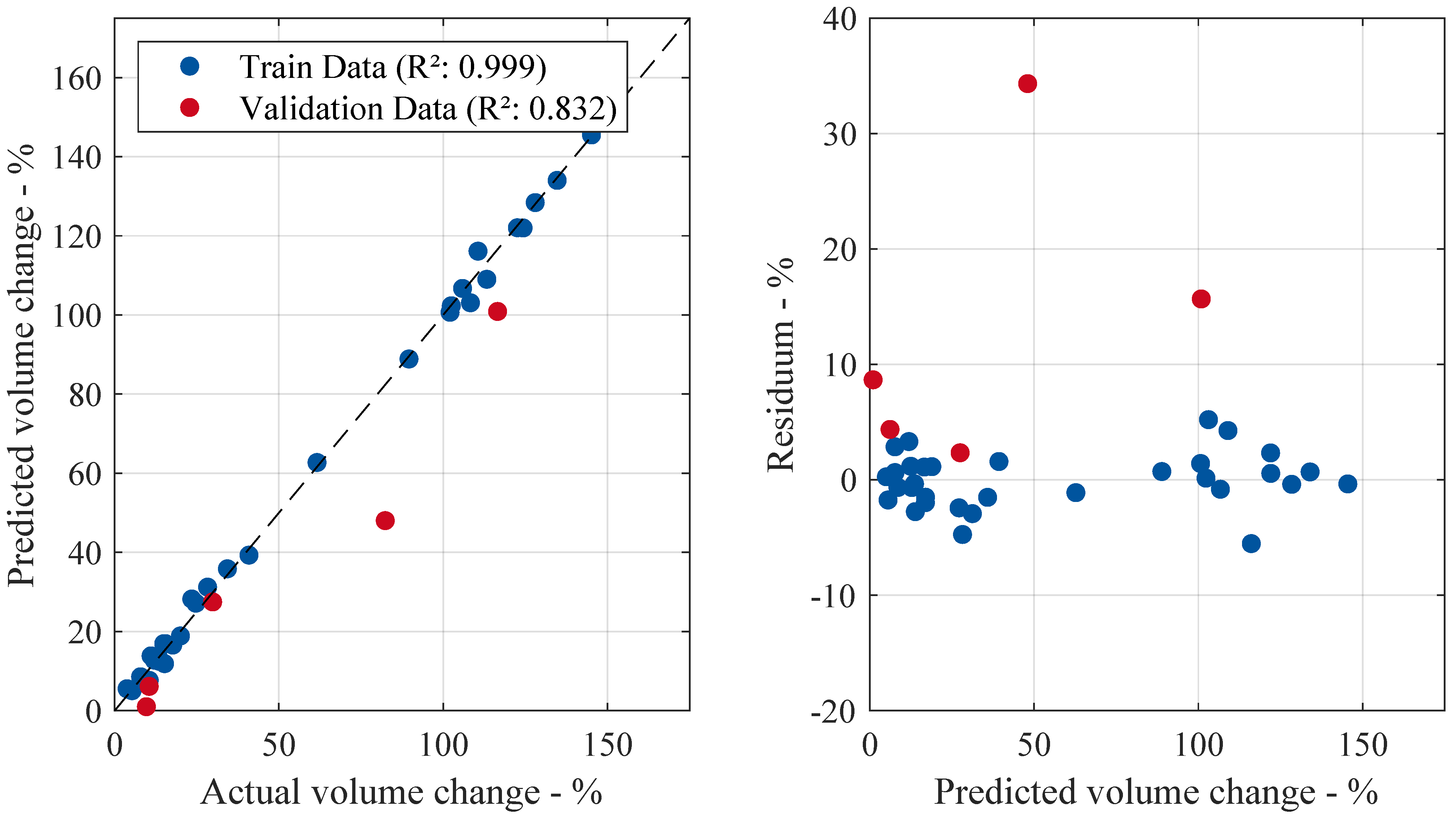
Figure 4 compares the predicted volume change to the actual values on the right-hand side during the training and validation process. Conversely, the residuals—the difference between the actual and predicted volume change—are plotted against the predicted values. A training $R^2$ score of $0.999$ indicates that the model was effectively trained using the available features and samples. The high validation $R^2$ score of $0.832$, close to the training score, indicates good predictive accuracy and generalization ability. Both scores are visually represented in the left scatter plot, where the data points closely align with the diagonal line, indicating near-ideal predictions with an $R^2$ value approaching one. Furthermore, the right-hand side of the figure shows that volume predictions changing up to around $50\%$ exhibit low residuals. Beyond this threshold, the residuals tend to increase, especially for the validation case, although no clear pattern emerges. 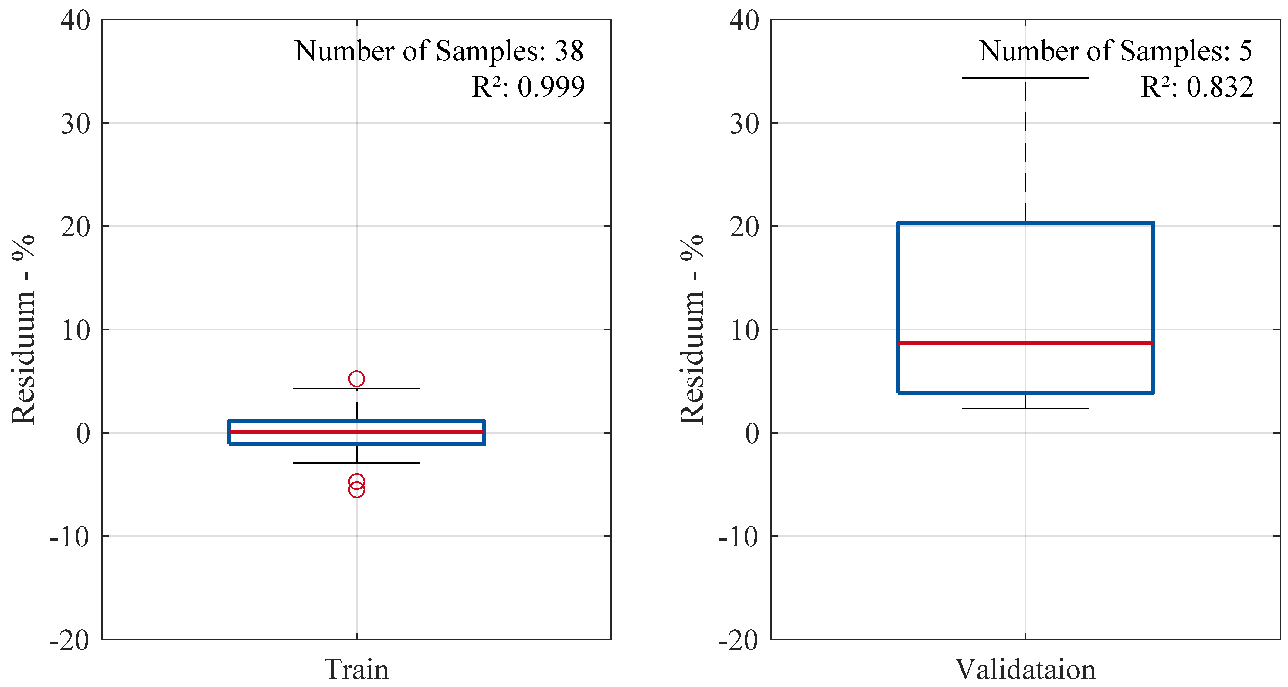Figure 5 presents box plots of the residuals for both the training and validation datasets. The distribution of residuals in the training set appears tightly clustered around zero, indicating a well-fitted model. Most predictions deviate by less than $\pm 4$ percentage points from the actual values. The validation residuals show a wider spread with a shift to positive values, with the median at $8.6\%$. This still suggests good generalization with minimal bias. However, it becomes evident that the outlier in the validation set, with an actual volume change of $82\%$ (2-octanone), exhibits the highest prediction error. This is due to a lack of training samples in this range of volume change. The model demonstrates stability and reliable predictive performance within the range of sufficient training data.

Overall, the selected HSP features and the chosen regression model and architecture demonstrate promising results during training and validation. To generate synthetic data that can be incorporated into the existing experimental dataset, the trained model was applied to a set of 59 untested substances. The relevant HSP features were collected for each of these substances, and the volume change was predicted based on those features. A summary of the substances and their corresponding predicted values is provided in

Table 6. Collection of substances with predicted volume change.

Name	CAS	HSP				Predicted
		${\mathit{\delta }}_{\mathit{D}}$	${\mathit{\delta }}_{\mathit{P}}$	${\mathit{\delta }}_{\mathit{H}}$	${\mathit{V}}_{\mathit{M}}$	$\mathbf{\Delta }{\mathit{V}}_{\mathit{pred}}$
		$\mathbf{\left[}{\mathbf{MPa}}^{\mathbf{1}\mathbf{/}\mathbf{2}}\mathbf{\right]}$	$\mathbf{\left[}{\mathbf{MPa}}^{\mathbf{1}\mathbf{/}\mathbf{2}}\mathbf{\right]}$	$\mathbf{\left[}{\mathbf{MPa}}^{\mathbf{1}\mathbf{/}\mathbf{2}}\mathbf{\right]}$	$\mathbf{\left[}{\displaystyle \frac{{\mathbf{cm}}^{\mathbf{3}}}{\mathbf{mol}}}\mathbf{\right]}$	[%]
1,4-Dioxane	123-91-1	17.5	1.8	9	85.7	85.33
1-Nitropropane	108-03-2	16.6	12.3	5.5	89.5	108.14
1-Pentanol	71-41-0	15.9	5.9	13.9	108.6	16.45
1-Propanol	71-23-8	16	6.8	17.4	75.1	7.97
2-Butanol	78-92-2	15.8	5.7	14.5	92	25.85
2-Phenoxy ethanol	122-99-6	17.8	5.7	14.3	124.7	58.69
Acetonitrile	75-05-8	15.3	18	6.1	52.9	103.39
Amyl acetate	628-63-7	15.8	3.3	6.1	148	66.19
Benzyl benzoate	120-51-4	20	5.1	5.2	190.3	106.41
Butyl Benzoate	136-60-7	18.3	5.6	5.5	178.1	76.37
Butyl diglycol acetate	124-17-4	16	4.1	8.2	208.2	11.71
Butyl glycol acetate	112-07-2	15.3	7.5	6.8	171.2	2.12
Chloroform	67-66-3	17.8	3.1	5.7	80.5	139.44
Diacetone alcohol	123-42-2	15.8	8.2	10.8	124.3	11.55
Diethyl ether	60-29-7	14.5	2.9	4.6	104.7	80.49
Diethylene glycol monomethyl ether	111-77-3	16.2	7.8	12.6	118.2	10.61
Di-isobutyl ketone	108-83-8	16	3.7	4.1	177.4	33.78
Dimethyl formamide (DMF)	68-12-2	17.4	13.7	11.3	77.4	111.89
Dimethyl sulfoxide (DMSO)	67-68-5	18.4	16.4	10.2	71.3	157.91
Dipropylene glycol methyl ether	112-28-7	15.5	5.7	11.2	156.1	18.10
D-Limonene	5989-27-5	17.2	1.8	4.3	162.9	65.92
Ethyl lactate	97-64-3	16	7.6	12.5	115	12.22
Ethylene carbonate	96-49-1	18	21.7	5.1	66	155.83
Ethylene glycol monobutyl ether	111-76-2	16	5.1	12.3	132	23.19
Gamma-butyrolactone (GBL)	96-48-0	18	16.6	7.4	76.5	153.86
Glycerol carbonate	931-40-8	17.9	25.5	17.4	83.2	66.08
Hexane	110-54-3	14.9	0	0	131.4	2.76
Isoamyl acetate	123-92-2	15.3	3.1	7	150.2	77.93
Isoamyl alcohol (3-methyl-1-butanol)	123-51-3	15.8	5.2	13.3	109.3	28.62
Isobutyl alcohol	78-83-1	15.1	5.7	15.9	92.9	14.61
Isobutyl isobutyrate	97-85-8	15.1	2.8	5.8	169.8	62.45
Isophorone	78-59-1	17	8	5	150.3	56.78
Isopropyl acetate	108-21-4	14.9	4.5	8.2	117.1	90.51
Isopropyl ether	108-20-3	15.1	3.2	3.2	141.8	52.29
M-cresol	108-39-4	18.5	6.5	13.7	105	135.73
Methyl acetate	79-20-9	15.5	7.2	7.6	79.8	113.65

and

Table 7. Continuation of Table 6.

Name	CAS	HSP				Predicted
		${\mathit{\delta }}_{\mathit{D}}$	${\mathbf{\delta }}_{\mathit{P}}$	${\mathit{\delta }}_{\mathit{H}}$	${\mathit{V}}_{\mathit{M}}$	$\mathbf{\Delta }{\mathit{V}}_{\mathit{pred}}$
		$\mathbf{\left[}{\mathbf{MPa}}^{\mathbf{1}\mathbf{/}\mathbf{2}}\mathbf{\right]}$	$\mathbf{\left[}{\mathbf{MPa}}^{\mathbf{1}\mathbf{/}\mathbf{2}}\mathbf{\right]}$	$\mathbf{\left[}{\mathbf{MPa}}^{\mathbf{1}\mathbf{/}\mathbf{2}}\mathbf{\right]}$	$\mathbf{\left[}{\displaystyle \frac{{\mathbf{cm}}^{\mathbf{3}}}{\mathbf{mol}}}\mathbf{\right]}$	[%]
Methyl cyclohexane	108-87-2	16	0	1	128.2	7.76
Methyl ethyl ketone (MEK)	78-93-3	16	9	5.1	90.2	105.02
Methyl isoamyl ketone	110-12-3	16	5.7	4.1	141.3	65.96
Methylisobutyl carbinol	108-11-2	15.4	3.3	12.3	127.2	55.44
Methyln-propyl ketone	107-87-9	16	7.6	4.7	107.3	93.98
Methylene dichloride (dichloromethane)	75-09-2	17	7.3	7.1	64.4	182.18
N,N-dimethyl acetamide	127-19-5	16.8	11.5	10.2	93	80.03
N-butyl acetate	123-86-4	15.8	3.7	6.3	132.6	77.78
N-butyl propionate	590-01-2	15.7	5.5	5.9	149.3	47.53
N-methyl-2-pyrrolidone (NMP)	872-50-4	18	12.3	7.2	96.6	152.42
N-propyl acetate	109-60-4	15.3	4.3	7.6	115.8	92.02
N-propyl propanoate	106-36-5	15.5	5.6	5.7	132.5	71.56
Propylene glycol monobutyl ether	5131-66-8	15.3	4.5	9.2	132	69.61
Propylene glycol monoethyl ether acetate	54839-24-6	15.6	6.3	7.7	155.1	20.91
Propylene glycol monomethyl ether	107-98-2	15.6	6.3	11.6	98.2	48.11
Propylene glycol monomethyl ether acetate	108-65-6	15.6	5.6	9.8	137.1	39.25
Propylene glycol monophenyl ether	770-35-4	17.4	5.3	11.5	143.2	48.62
P-xylene	106-42-3	17.6	1	3.1	123.9	96.26
Sec-Butyl Acenineate	105-46-4	15	3.7	7.6	134	87.88
Sulfolane (tetramethylene sulfone)	126-33-0	18	18	9.9	95.3	100.59
T-butyl acetate	540-88-5	15	3.7	6	134.8	82.23
Tetrahydrofuran (THF)	109-99-9	16.8	5.7	8	81.9	141.98
Tetrahydrofurfuryl alcohol	97-99-4	17.8	8.2	12.9	97.4	110.36

. It is important to note that no data validation is available at this stage, as no experimental investigations have been conducted for these substances yet.

The addition of simulation more than doubles the sample size, which can enhance the predictive accuracy of the framework presented above without the need for time-consuming immersion tests. Before exploring the impact of an expanded database on prediction accuracy, a baseline performance is established using only the experimental results.

3.2. Baseline Results

To establish a baseline score for comparison and assess whether the newly generated data impact the accuracy of the prediction framework, the model was first trained using only the available experimental data. This section presents the results of the baseline case. For this purpose, four standard regression models are evaluated: linear regression (Linear), lasso regression (Lasso), multilayer perceptron (MLP) regression, and tree-based regression (Tree). All four models are integrated into the prediction framework, with data preprocessing applied uniformly across the entire dataset. Each model is then individually optimized using halving grid search CV to determine the best hyperparameters. Finally, the optimal models are trained and evaluated using 5-fold cross-validation.

The models’ performances were evaluated during training and testing using the coefficient of determination $R^2$. Additionally, residual values—the differences between the actual and predicted volume changes—were calculated for each sample in both phases. The distribution of residuals is visualized using a box plot. As the previous chapter shows, the box plot effectively summarizes other representations, such as scatter plots of actual vs. predicted values or residuals, providing a comprehensive overview of model performance. Hence, this method of presentation is chosen for model comparison. All models are trained using 39 samples, while the remaining 10 are reserved for testing. The optimal hyperparameters, determined through hyperparameter tuning, are presented in

Table 8. Summary of optimal hyperparameters for baseline investigation.

Lasso	MLP	Tree-Based
Alpha: $0.1$	Alpha: $0.0001$	Max depth: 16
Tolerance: $0.01$	Solver: adam	Max features: log2
	Activation: tanh	Min sample leaf: 2
	Hidden layer sizes: (2,)	Min sample split: 2
	Learning rate init: 0.1
	Max iterations: 3000

. Since the linear model omits adjustable hyperparameters, it is excluded from the table.

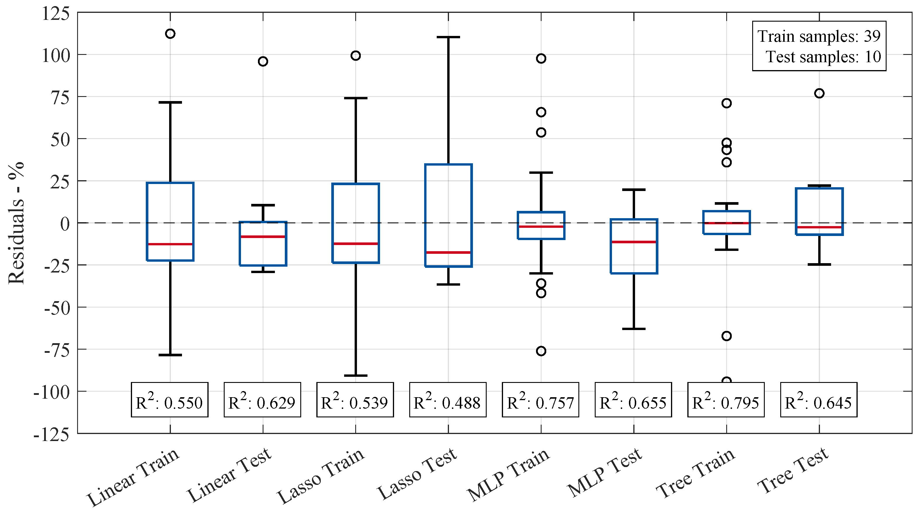
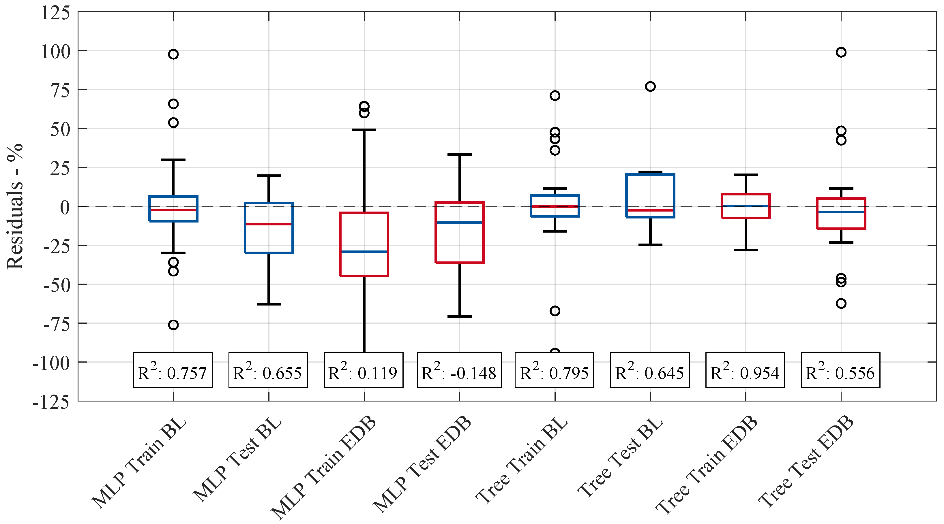
Figure 6 presents box plots of the residuals for all investigated regression models, comparing both training and testing phases. The distribution of residuals provides insight into each model’s predictive performance, with a narrower spread indicating higher accuracy. This figure highlights variations in model stability and generalization ability by visualizing the differences between the actual and predicted volume changes.

The median residuals for each model remain close to zero, indicating minimal bias towards larger prediction values. However, the variation in residual spread suggests that specific models exhibit more stability in their predictions than others. The range of residuals highlights differences in the models’ predictive reliability, with some models demonstrating more significant variation in errors across the data points, indicating less consistency in their performance. The MLP and tree-based models showed the highest $R^2$ values, with training scores of $0.757$ and $0.795$, respectively, and testing scores of $0.655$ and $0.645$, respectively. These results suggest that both models achieve a good fit for the training data and good generalization of unseen test data. However, outliers in the data still affect model performance, as their influence can lead to deviations in both the training and testing results. Despite this, the range of predicted values (minimum and maximum) remained almost consistent across all models, indicating that the models were similarly constrained in the spread of their predictions. In contrast, the linear and Lasso models yielded lower $R^2$ values and thus lower predictive accuracy. These models appear to underfit the data, as their relatively simple structure fails to capture the underlying complexity of the relationships in the dataset given the available describing features and number of samples. This results in less-accurate predictions on both the training and testing sets. Notably, none of the models achieved sufficiently high training $R^2$ values, implying that the selected molecular descriptors, alongside the limited amount of data samples, do not fully capture the underlying patterns in the data. This limitation in feature representation leads to insufficient model training, which in turn adversely affects performance on the test set. Consequently, the linear model’s better performance during testing may be attributed to chance rather than a robust generalization ability.

An increase in predictive accuracy is expected with a larger dataset. Therefore, this study explores alternative approaches to experimental testing for generating new data samples. In the following, the database is expanded by incorporating samples whose elastomer volume change has been predicted using the HSP approach and a regression model.

3.3. Expanded Database Results

This section examines the impact of a larger dataset by comparing the prediction accuracy of the expanded and baseline cases. First, the models were evaluated using the same hyperparameters as in the baseline case. In the second step, new hyperparameters optimized for the expanded dataset were applied to assess potential improvements in predictive performance. The total number of samples, including the newly generated data, amounted to 108. However, some outliers were removed due to constraints related to technical plausibility, resulting in a final dataset of 95 samples. As before, 5-fold cross-validation was performed, yielding 76 training samples and 19 testing samples per fold. Figure 7 compares the residual values and $R^2$ scores of all investigated models in the baseline case with those obtained using the expanded database. At this stage, the models in both cases share the same hyperparameters from Table 8.

Expanding the dataset shifts the median residuals closer to zero for most models (Linear, Lasso, and tree-based) compared to the baseline case. However, across all the models, the $R^2$ scores decrease, except for the tree-based model in training, which slightly improves ($R^2=0.795$ for BL, $R^2=0.954$ for EDB). This indicates a reduction in predictive accuracy for the other models. The tree-based model demonstrates greater robustness, maintaining stable or even improved performance. On the other hand, the MLP model exhibits significant instability, characterized by wider residual spreads and even a negative testing $R^2$ score.

The results suggest that while increased data volume can improve model training, it may also introduce complexities that negatively impact certain model architectures, particularly those more sensitive to data distribution changes. Therefore, it is essential to adjust the model architecture, where possible, to one that is optimally suited to the characteristics of the given dataset. Thus, in the following analysis, the models are re-optimized for the dataset by individually tuning their hyperparameters to improve performance and adaptability.

The following section presents the model performance results after re-optimizing the hyperparameters for the extended database case. Since the dataset size nearly doubled, each model’s architecture was individually adjusted to accommodate the increased data complexity. The resulting optimal hyperparameters are summarized in

Table 9. Summary of optimal hyperparameters for extended database investigation.

Lasso	MLP	Tree-Based
Alpha: 1	Alpha: 0.001	Max depth: 64
Tolerance: 0.0001	Solver: $adam$	Max features: $sqrt$
	Activation: $tanh$	Min sample leaf: 8
	Hidden layer sizes: (2,)	Min sample split: 2
	Learning rate init: 0.1
	Max iterations: 10,000

. Furthermore, the number of input features was increased from five to seven to accommodate the larger dataset better and capture additional patterns in the data.

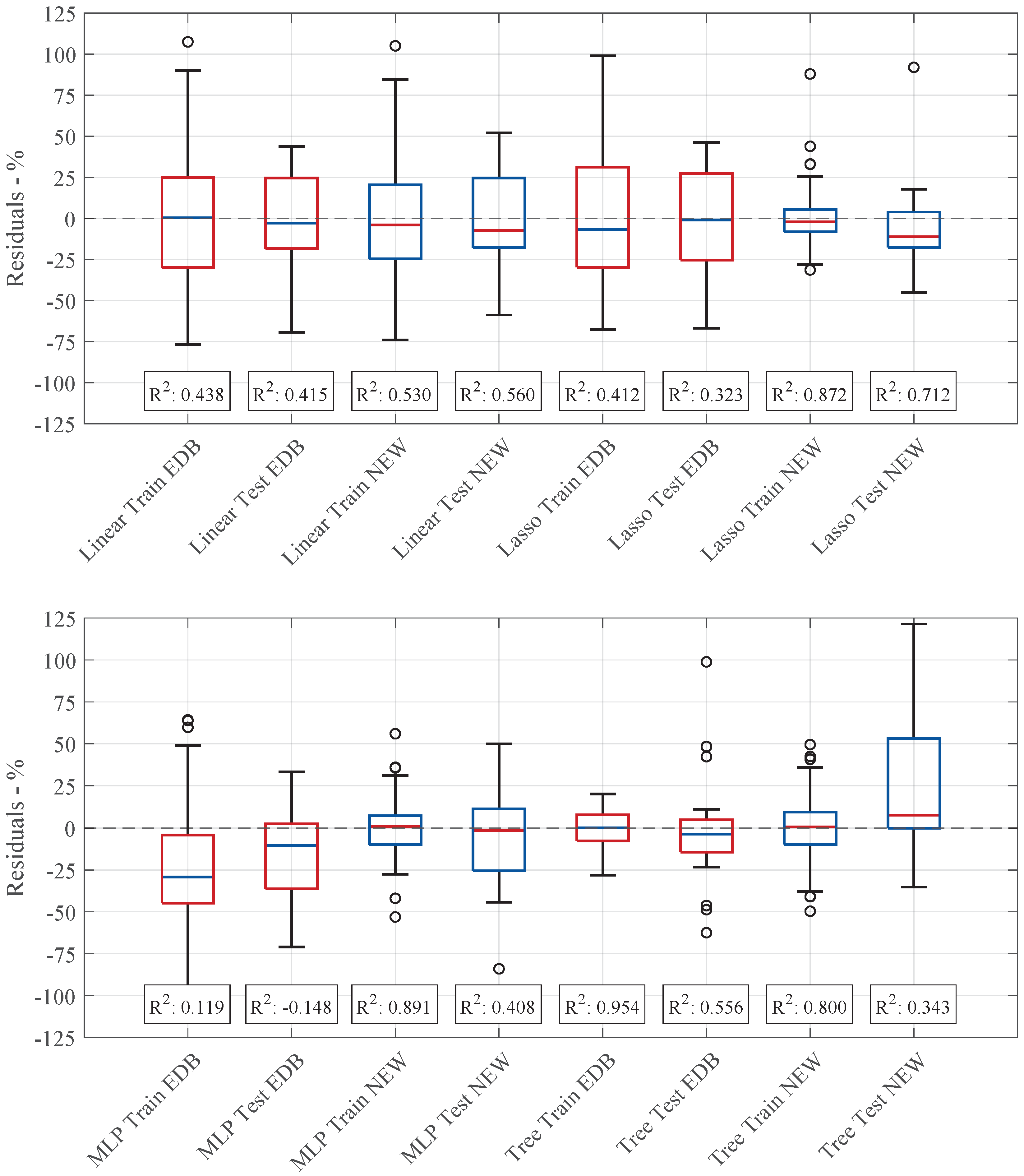
Figure 8 shows the residual distributions and $R^2$ scores for training and testing across the different models, comparing their performance before and after hyperparameter optimization. While some models showed significant improvements, others experienced a decline in predictive accuracy, indicating that the effects of dataset expansion and parameter tuning varied depending on the model architecture.

For example, the linear model slightly improved, with a lower median residual and reduced spread in the updated configuration. This led to a modest increase in the $R^2$ score, rising from $0.438$ to $0.530$ in training and from $0.415$ to $0.560$ in testing. However, the overall performance remained moderate, with $R^2$ values of around $0.5$. Since the linear model lacks adjustable hyperparameters, these improvements were primarily attributed to the increased dataset size and additional input features. The lasso regression model showed an apparent enhancement in predictive performance. The residual spread was significantly reduced, though some outliers remained present. The $R^2$ score improved considerably, increasing from $0.412$ to $0.872$ in training and from $0.323$ to $0.712$ in testing. Additionally, the median residual deviation in testing was close to zero, suggesting better model fit and improved generalization. The MLP regression model demonstrated the most substantial improvement. The training $R^2$ score rose from $0.119$ to $0.891$, while the testing $R^2$ improved to $0.408$. The residual distribution became more centered, with the median closer to zero, and the overall spread was reduced, particularly in training. However, despite these gains, the testing performance still exhibited a relatively wide residual distribution, indicating persistent instability in generalization. Conversely, the tree-based regression model experienced a decline in performance. While the spread of residuals increased in training, the interquartile range remained nearly unchanged. The training $R^2$ decreased from $0.954$ to $0.800$, showing fewer signs of overfitting than before. However, testing performance deteriorated, shifting residual distribution toward positive values and increasing prediction errors. The testing $R^2$ dropped from $0.556$ to $0.343$, indicating reduced generalization capability.

The results highlight that while hyperparameter tuning leads to substantial improvements for the MLP and lasso models, the tree-based model showed a decline in predictive performance. The linear model benefited slightly from the increased dataset, whereas the MLP model, despite achieving substantial improvements in training, still faced challenges in stability during testing. These findings emphasize the need for model-specific optimizations and careful consideration of dataset expansion effects when adjusting model architectures. No uniform statement can be made by comparing the prediction accuracy based on the $R^2$ score and the residual distribution of the old and new architecture.

4. Discussion

In this study, two approaches were investigated for modeling intermolecular interactions between fuel and sealing materials. However, only one approach demonstrated applicability across a wide range of fuel candidates. The decision to focus solely on the HSP approach was based on the Pearson correlation coefficient. As shown in Table 4, the HSP variables exhibited a stronger overall correlation with volume change compared to the DFT variables. Interestingly, when considering only alcohol-based fuels, the correlation score for the DFT variables increased significantly. This finding aligns with the results reported by Yamada et al. [32], which initially motivated the evaluation of the DFT approach. However, a key limitation of the DFT method is its inability to account for functional groups beyond alcohols, restricting its applicability in this study.

A possible explanation for the poor performance of the DFT approach is that it may not adequately capture the relevant binding interactions between the fuel candidate and NBR. For example, in systems containing alcohols, a distinct hydrogen bond forms between the hydrogen atom on the fuel and the nitrogen atom on the NBR. For compounds lacking an OH group, the formation of such bonds is less evident, suggesting that hydrogen bonding is not the predominant interaction driving elatomer volume change in these cases. It is plausible that, for these other molecules, alternative binding sites with more favorable interactions exist but were not identified by the algorithm. This limitation may be partly due to the initial conditions used for geometry optimization. Adjusting these conditions could lead to different binding configurations and potentially improve the accuracy of the DFT approach.

By choosing the HSP approach, the volume change database was extended via a regression model. However, the dataset available for this process was limited. Despite this constraint, the selected model architecture yielded near-optimal prediction accuracy during training. Nonetheless, the slightly lower accuracy observed during validation suggests a tendency toward overfitting, thereby reducing model robustness. When the trained model was applied to previously unseen data, this overfitting introduced additional uncertainty in the predictions. Furthermore, these predictions could not be directly validated against experimental values due to the nature of the process. An analysis of the validation residuals in Figure 4 reveals that, in regions with sufficient training data, most predictions deviated by less than $10\%$ from the actual values.

Although this study prioritized rapid and reproducible experimental execution, previous investigations in the literature (e.g., ref. [50]) have shown that the extent of elastomer property change is highly sensitive to the experimental setup and manual execution. In this context, the relevant DIN standard [34] recommends fast execution of manual measurements without specifying a precise time frame. Moreover, the high volatility of most substances examined further complicates the acquisition of precise and reproducible measurements, particularly when multiple operators are involved. The resulting specimen-to-specimen measurement error is comparable in magnitude to the model’s predictive uncertainty. For example, in three previous immersion tests, the mean relative deviation was found to be $4.61\%$ for NBR in ethanol and $12.49\%$ for NBR in methanol. These considerations therefore underscore the validity of incorporating simulated data into the prediction framework central to this study.

This study investigates the impact of simulated data on the predictive accuracy of volume change. By comparing the prediction accuracy of models trained on the extended database to those trained on the baseline dataset, several key observations can be made. As discussed in the results section, simply increasing the number of data samples does not necessarily improve model performance. In fact, most models—except for the tree-based regression model—exhibit a decline in predictive accuracy when additional data are introduced. This highlights the need to adjust both the model architecture and the number of molecular input descriptors to effectively accommodate the larger dataset. Only through such modifications does prediction accuracy return to baseline levels or, in some cases, surpass previous performance. However, it is important to note that no model, except for the Lasso regression model, demonstrates significant improvement, and testing accuracy is almost always lower than training accuracy.

Two possible explanations for this trend likely contribute simultaneously. The first is the aforementioned increase in uncertainty introduced by the simulated data. The second is the small dataset, despite the addition of new samples. Clear signs of underfitting were evident, which could be attributed to the limited dataset size. While underfitting is expected to decrease as the number of data samples increases, the nearly equal ratio of experimental to simulated data may amplify uncertainty propagation from the simulated data into the model predictions. To mitigate this effect, a lower ratio of simulated to experimental data could be implemented, as explored by Makansi et al. [19].

At this stage, the limited dataset size remains a key factor preventing definitive conclusions about model performance. While trends in predictive accuracy could be observed, the dataset is not yet large enough to allow for a clear and statistically significant comparison between models. Some models show promising behavior, but the variability in results suggests that further data collection trough experiments is necessary to fully assess their reliability.

5. Conclusions

Within the context of the fuel design process at the Cluster of Excellence “The Fuel Science Center”, the material compatibility of elastomers and bio-hybrid fuels was investigated. By analyzing changes in elastomer properties after being immersed in bio-hybrid fuels, underlying patterns could be identified. These results enable the development of recommendations for future applications, such as optimizing fuel blend compositions to improve compatibility with existing combustion engine sealing systems.

To reduce the the reliance on further time-consuming and costly experimental investigations, a data-driven approach was developed to predict elastomer property changes after fuel immersion. This approach was implemented through a prediction framework that utilizes supervised learning regression models to identify patterns within the available experimental data. The models were trained on molecular fuel parameters alongside corresponding property changes and were subsequently applied to previously untested substances to generate new predictions. However, an initial evaluation of the framework revealed that the limited dataset size led to non-robust predictions and a lack of statistically significant accuracy across the investigated models [9].

To address these limitations, this work explored methods to generate synthetic data for integration into the existing experimental dataset. The data generation strategies focused on modeling intermolecular interactions between fuel candidates or pure fuel constituents and elastomer materials. Two approaches were considered: a detailed density functional theory method and a more abstract approach based on Hansen solubility parameters combined with a regression model. A key objective of this work was to assess the impact of the extended database on the performance of the prediction framework.

Among the two methods, the HSP approach yielded more promising results and was subsequently used to double the number of data samples. Although the data generation process achieved high prediction accuracy, it inherently introduced uncertainty, since the newly generated data could not be directly validated against experimental measurements. The HSP approach was favored due to the widespread availability of HSPs in the literature, whereas DFT calculations are computationally intensive and proved applicable only to substances of the functional group of alcohols. The effects of the extended database on prediction accuracy were evaluated by comparing the baseline case, which contained only experimental data, with the extended dataset. Both the coefficient of determination and the residual distributions during training and testing were analyzed. The findings indicated that simply adding simulated data without adjusting model hyperparameters did not enhance model accuracy or robustness. Only after re-optimizing the hyperparameters to accommodate the larger dataset did the performance reach, or even exceed, the baseline levels. Nevertheless, a significant gap between training and testing accuracy suggests that the models continue to underfit the data. This is likely due to the uncertainty introduced by integrating simulated volume change data in an equal proportion to the experimental data. In combination with the still small dataset, this results in an unfavorable generalization ability. Another, though at this stage less prominent, reason might be that the chosen molecular descriptors do not fully capture the key factors influencing elastomer volume change.

Overall, the developed framework provides a scalable solution, enabling the efficient incorporation of additional data. As the database expands, the robustness of the models is expected to improve, allowing for more precise evaluations and potentially stronger predictive performance in future studies. It is therefore necessary to conduct further experiments to expand the database without introducing uncertainty from simulated data. Also, future research will focus on fine-tuning the balance between experimental and simulated data. Additionally, the potential benefits of directly incorporating HSP values as input parameters into the prediction framework warrant further investigation.