Soil Carbon Remote Sensing: A Meta-Analysis and Systematic Review of Published Results from 1969–2022

Abstract

Soil carbon remote sensing has become a popular topic amongst scientists, policy makers, landholders, and others in recent years, as pragmatic perspectives on climate change, land productivity, and food security become increasingly important. Unfortunately, more than fifty years of existing research has not provided clarity or consensus on the best soil carbon remote sensing methods. A reliable, widely applicable, robust, and cost-effective means of soil carbon modelling remains elusive. As evidenced by aggregated data from 259 papers and 503 models published since 1969, much experimentation has been undertaken and soil carbon remote sensing shows promise, but the situation remains unresolved. First, this review and meta-analysis shows that soil carbon remote sensing model accuracy (via Pearson’s correlation coefficient R²) has decreased on average since 1969, and more rapidly since the year 2000. Second, the model R² does not correlate strongly with the spatial (airborne platforms compared with satellite platforms) or spectral (multispectral compared with hyperspectral) resolution of data. Third, no significant relationship between the model R² and the number of samples included in the training/test dataset is apparent. Fourth, the R² of non-parametric models (mean R² in 2022 = 0.58, n = 117) has declined more rapidly (decrease of 1.3% per year) since 1969 (mean R² in 1969 = 0.74, n = 1) than the R² of parametric models (decrease of 0.4% per year), suggesting that the algorithm applied during soil carbon modelling may be of importance. Finally, data compiled in this meta-analysis demonstrate a correlation between declining model R² and the increased use of satellite multispectral data and non-parametric algorithms, particularly machine learning, since the year 2000. There is no other evidence to suggest that prediction models prepared with multispectral data perform worse than other models, however. Hence, for the purpose of experimentation, it may be valuable to continue experimenting with the use of machine learning models for soil carbon prediction. However, when model performance is the priority, it is recommended that simple, parametric models (such as linear regression) are applied.

1. Introduction

Soil Organic Carbon (SOC) is a critical component of healthy, drought-resilient, and productive soils [1,2]. In agricultural settings, SOC is often considered a robust indicator of soil fertility [3,4]. However, in order to manage SOC stocks, practical, reliable, and affordable SOC measurement and monitoring techniques are required [5,6]. The measurement and monitoring of SOC is also relevant to climate change mitigation [7,8], with many countries eager to offset some domestic emissions with improvements in SOC in order to meet their commitments or targets under the Paris Climate Agreement [9]. If undertaken effectively, efficiently, and fairly, carbon trading schemes have the potential to benefit all directly involved, as well as the wider community, by improving domestic food security [10], decreasing soil erosion [11], reducing dust emissions [12], and improving drought resilience [13].

Though SOC has attracted strong interest and investments from governments, private industry, and landholders [7,14] in the past 5 years as these parties consider the legitimate associated economic, strategic, and climate change mitigation opportunities [15], an efficient, widely-applicable, reliable, and cost-effective method for measuring or monitoring soil organic carbon remains elusive. Industry-standard laboratory-based SOC testing remains expensive, labour-intensive, and impractical for many scenarios [16]. Though numerous efforts have been made to provide alternative monitoring solutions (such as the use of spectroscopic models for SOC quantification in the Australian ACCU Methodology [17]), none of these approaches appear to substantially reduce the time, effort, or expense of monitoring SOC stocks. By comparison, soil carbon remote sensing would revolutionise soil carbon monitoring across the world if a reliable, replicable, and widely applicable approach was identified, demonstrated, and validated.

A number of authors have claimed that there were few soil carbon remote sensing studies published prior to the mid 2010s, due to “complexities involved in the acquisition of reflectance data” [18] and other such challenges. By contrast, a proliferation of soil carbon remote sensing studies, reviews, and experiments have occurred in recent years [19]. Nonetheless, the best methods, platforms, sensors, algorithms, and number of samples required to construct a robust model remain unclear. In an attempt to address this problem, this paper presents a meta-analysis of soil carbon remote sensing studies published since 1969.

The authors would like to recognise a number of other review papers which address the topic of SOC remote sensing, at least partially. We start by addressing them.

In 2019, Nayak et al. published a review of current and emerging analytical methods for SOC monitoring. Laboratory-based, aerial spectroscopy (remote sensing), and other modelling approaches were included. The review concluded that the eddy-covariance approach (which uses a range of data sources to measure the net ecosystem exchange, production, carbon sequestration, and greenhouse gas emission) and agricultural life cycle assessments were currently the most appropriate monitoring methods at an ecosystem level. However, it was also hypothesised that as the signal-to-noise ratio of hyperspectral sensors improved, the prediction accuracy of models constructed with data from these platforms would also improve.

In a comprehensive review of geospatial technologies available for assessment of carbon stocks, Dahy, Issa [20] reported that remote sensing was effective for saving time and money when mapping carbon stocks, but required additional field data and sample data to be effective. By contrast, it was also reported that remote sensing technology was extremely expensive. The review did not clarify which of these perspectives was the dominant view. Regardless, it could be argued that the latter point is becoming increasing irrelevant through time, as modern software and research efforts have substantially reduced the effort and cost involved in the collection, processing, and application of remote sensing data. For example, high-resolution, pre-processed Sentinel-2 data are freely available for download, or modelling within Google Earth Engine. Hopefully, such advances have meaningfully reduced the cost, expertise, and data availability barriers for SOC remote sensing. Substantial reductions in the cost of obtaining ground-truth sample data would further allow any interested parties to partake in SOC mapping and modelling activities in the future.

In a systematic review of earth observation-driven soil monitoring studies published in international journals between 2019 and 2021, Tziolas et al. [21] identified 46 peer-reviewed articles. Articles were found using the keywords “Soil” AND “Blockchain” OR “Citizen Science”, with 33 referring to SOC monitoring. The review identified data sharing, thresholding for bare soil detection, the under-utilisation of existing infrastructure, and the effect of soil surface conditions (roughness, crusts, and soil moisture content) as the main limitations to effective mapping of soil properties. The review concluded that the best opportunities for future earth observation data-driven soil mapping stemmed from the use of artificial intelligence, the sharing of labelled model training datasets, and fusing data from ground and remote sensing platforms. Technological advancements in data processing and sensor resolution were also predicted to improve soil monitoring outcomes, as were overcoming political and financial issues experienced in preparing comprehensive training and test datasets. It was suggested that these improvements may help to overcome some of the current barriers for interdisciplinary research and multi-actor coordination in this field. No aggregated results were presented.

In two review papers concerning the utility, challenges, and prospects of basic and deep learning models applied to SOC prediction models utilising remotely-sensed data, Odebiri, Mutanga [15] and Odebiri, Odindi [22] highlighted the logistical and technological challenges associated with SOC remote sensing. Specifically, the long processing time and significant infrastructure required to process high-dimensional data incorporating spatial, temporal, and spectral variables, which are required for deep-learning models. Suggestions provided included the use of Extreme Machine Learning algorithms, which pool data to reduce dimensionality, to improve the speed and efficiency of calculations.

Odebiri et al. [15] identified that the “overall accuracy” (as measured by the standard Pearson correlation coefficient R², used throughout this review) of prediction models was higher when hyperspectral data was utilised. Moreover, model accuracy improved for deep-learning algorithms when more samples were utilised and the model R² values for artificial neural networks were lower than stochastic gradient boosting, random forest, and support vector machine regression when less than 100 samples were utilised. All results suggested that more complex machine learning (ML) algorithms with higher numbers of layers perform better when more data is incorporated. This, in turn, causes problems with the speed and efficiency of calculations.

Vaudour et al. [23] published an overview of organic carbon modelling with satellite remote imagery over cultivated areas. The overview covered studies published since 1990, with most study sites in Europe, China, and North America. Partial Least Square Regression (PLSR), Random Forest (RF), or other ML models such as Support Vector Machine (SVM) were the most commonly applied prediction algorithms. It was reported that most studies relied upon spatial interpolation of SOC across the study area, following SOC prediction over bare soil areas. Bare soil areas were typically identified with Normalised Difference Vegetation Index (NDVI) thresholding, and anywhere between 32 and 1753 soil samples were utilised in construction of the SOC predictive models.

Chen, Arrouays [24] presented a review of 244 Digital Soil Mapping (DSM) articles published between January 2003 and July 2021 which considered soil DSM on areas > 10 × 10⁴ km². DSM involves the development of landscape-based models relying on spatial interpolation of environmental factors such as terrain, climate, vegetation, and soil properties [25,26]. Most studies reviewed by Chen, Arrouays [24] were published by authors from China, France, Australia, or the USA, and approximately 78% of the articles (189) considered SOC or SOM. R² and RMSE were the primary error metrics used to compare studies, as they were most commonly reported. When multiple models were recorded in one paper, the details of each model were recorded. It was also reported that there had been a substantial increase in the use of ML models (defined as “non-linear models”) since the beginning of the study period and that the mean model R² for surface SOC DSM models was 0.51.

The present meta-analysis reviews, extends, and generalises the work of Chen, Arrouays [24] in several ways. Firstly, DSM and SOC remote sensing can be defined differently. Specifically, DSM activities do not necessarily involve remote sensing data. Instead, they more typically include environmental, climatic, geologic, and other spatial data layers, commonly including legacy or historical data Chen, Arrouays [24]. Hence, the present analysis includes studies from a much wider date range of 1969–2022, and is not limited to studies reporting on models applied to areas > 10⁵ km² which report based on “standard GlobalSoilMap [27] like depths”, and in the analysis section, algorithm “types” are grouped quite differently. DSM studies compiled by Chen, Arrouays [24] were mostly published by authors in China, France, Australia, or the USA, while SOC remote sensing studies included in this review were most commonly published by authors from Iran. This review also includes more studies (259 papers and 503 studies), though it solely considers articles presenting results for soil carbon predictive models derived from remote sensing data.

Other studies comparing selected satellite platforms [19], band combinations [28], spectral resolution [29], and spatial resolution [30] are also available. However, none of these studies provide comprehensive, quantitative insights into the most reliable, transferable, or robust methods suitable for application in a broad range of environments, climates, and landscapes. This study considers and analyses the model metrics (R²) of all studies reported in a paper, as well as the best model presented in a paper, where multiple studies are presented. Importantly, there were no significant changes in the results of our analyses when our model database was filtered to include only the best models from each paper (259 of 503 models).

As a point of difference to all of the SOC remote sensing reviews summarised above, this paper presents a meta-analysis, as defined by Harrer et al. [31], with clearly defined filtering criteria, reproducible methods, and the combining of data in a quantitative way. Hence, the search and filtering criteria applied, as well as the data preparation and manipulation steps, are detailed in the Methods section. Quantitative analyses of the “best” remote sensing platforms and algorithms for SOC modelling are presented in an attempt to quantitatively identify, highlight, and facilitate the application of effective SOC remote sensing strategies, thereby facilitating the acceleration of soil carbon monitoring and sequestration activities.

Following the Introduction, this review presents a detailed description of the methods, assumptions, and software tools applied to collect, analyse, and summarise data extracted from the 259 soil carbon remote sensing papers reviewed. In the Results section, summaries of publication statistics (publication year, remote sensing platform, model type etc.) are provided before quantitatively analysing the influence of various study parameters on model performance (R²). In the Discussion, these results are compared with insights from the literature and interrogated further. The Conclusion summarises the review’s analyses, results, and conclusions.

2. Materials and Methods

2.1. Paper Inclusion Criteria and Definition of R²

This meta-analysis focuses on the “best” methods, algorithms, platforms, and/or sensors for terrestrial soil carbon remote sensing studies. Studies from all regions and time periods were sought; hence, the search terms utilised were quite broad. However, studies considering wetland, mangrove, seagrass, peat bog, marsh, or near-shore coastal environments were excluded, as this review has a terrestrial focus.

Soil carbon is referred to in a number of different ways throughout the publications compiled. Although defined differently, soil organic matter is directly comparable to soil organic carbon and therefore of interest in this meta-analysis. Search terms entered into Web of Science reflected these similarities and were as follows: “SOC OR SOM” AND “remote sensing OR satellite OR UAV OR UAS” AND “carbon”. Initially, the additional criteria of “Soil organic carbon or soil organic matter” was included; however, this search returned 137,992 results and included a high proportion of irrelevant results, even once subject-specific filtering options were applied. Hence, the former search was applied.

The refined Web of Science search returned 3108 results. These entries were exported into Endnote and filtered according to their title and abstract. Where further clarification was required, the full paper was read to determine eligibility. Similar search terms were also entered into Google Scholar to identify any papers published in less well-publicised sources. A further 109 potentially relevant papers were identified in Google Scholar.

Following this initial filtering stage, the eligible paper count sat at 357. Additional filtering led to the removal of 22 papers which were identified as duplicates or presenting identical results as another paper. During further filtering, 43 papers were removed due to the absence of details regarding the algorithm used for model construction, a non-standard use of or lack of model R², or lack of definition of the remote sensing data collection platform. An additional 23 papers were removed due to their irrelevance to the study topic, i.e., modelling of above-ground biomass, deep carbon stores, erosion prevention, GIS modelling with no remote sensing data, moss extent, inorganic carbon stock, or carbon storage in a peat bog.

Papers published in conference libraries for which the full paper was not readily accessible [32], papers which described an upcoming experiment [33], used simulated [34,35] or synthetic data [36], used remote sensing platforms to collect data in the lab [37], or which were not available in English [38] were also not included. Overall, 259 papers, containing details of 503 studies, were included in the meta-analysis.

R² is defined as the square of Pearson’s Correlation Coefficient, sometimes now known as the “coefficient of determination” [39] but originally termed the “coefficient of correlation” [40]. It quantifies the degree of association between a model and a dataset [41]. Widely used to compare the performance of different models [42,43], there is no universal agreement for an R² threshold which indicates a “good” model [44]. R² is used here and commonly elsewhere to compare the performance of SOC remote sensing studies because it is the most frequently reported statistic in the database of compiled studies. A recent review of common statistics by Chicco, Warrens [43] also concluded the R² was more useful than RMSE, MSE, MAPE, MAE, and SMAPE to evaluate and compare the performance of regression and machine learning based analyses.

Unbiased splitting of test and training datasets should result in comparable statistical properties for both datasets. This implies that the values of R² between test and training datasets should be the same within uncertainty limits. With some studies only reporting one R² statistic or failing to clearly distinguish between the R² of model calibration and validation, the R² statistics reported for all studies are assumed to be comparable. The R² statistic considered for each publication and each model can be seen in the database of studies compiled for this review, available here, and are used in the analyses below.

2.2. Data Categorisation and Analysis

Details of the model type, data collection platform, and algorithm applied for model building were requirements in the filtering process, as these details were required for categorisation and thematic analysis of the data. Hence, each manuscript was manually searched to extract the required information. Details were recorded in an Excel spreadsheet which was used as a database for analysis (https://data.mendeley.com/datasets/zz4x7xkwkx/1, accessed on 5 February 2023). Since some papers presented results for multiple studies or models, the final database included details of 503 soil carbon remote sensing models.

Following compilation of the database, data visualisation and analysis were conducted in Python 3.10.9. Exploratory data analysis revealed the need to reduce the number of categories of sensors to ensure a representative sample in each category. Hence, sensors were classified according to their mounting platform (satellite or airborne) and the sensor resolution (hyperspectral or multispectral). The resulting categories are satellite multispectral (SatM), satellite hyperspectral (SatH), airborne multispectral (ABM), and airborne hyperspectral (ABH). In the analyses, interpretations presented, and discussion below, it is assumed that the spectral resolution of data collected with hyperspectral sensors is greater than for multispectral sensors, and that the spatial resolution of airborne sensor data is higher than that of satellite data.

For some results presented, especially where numerous data points overlapped, it was helpful to apply linear models to the data presented. This allowed determination of the existence or non-existence, and the strength and statistical significance, of a relationship between two variables. A number of linear models and their associated equations are presented below.

2.3. Other Variables and Information

If data from multiple sensors were included in the model, the study was categorised under the highest-resolution sensor. For example, Guo et al. [45] constructed a model combining hyperspectral data from the Headwall–Hyperspec (380–1700 nm) sensor with Sentinel-2 and Landsat 8 multispectral satellite data. The study was categorised as ABH, as the highest-resolution data incorporated in the model was hyperspectral data collected from an airborne platform.

Many studies described the use of multiple algorithms for building SOC prediction models. When multiple approaches were applied during the construction of a single model, only one algorithm was recorded. This practice was applied to avoid the use of many different categories with only one entry. Model type classifications were allocated in the following order: Kriging > Bayesian > PLSR > PCA & Puchwein > Machine Learning > Linear Regression > Other Regression > Map/Layer algebra & HYSOMA. For example, if a model applied Bayesian kriging, the study was classified as a kriging study.

When results were presented for a number of model types (linear, non-linear, ML, etc.), results from each model were included in the database in most cases. However, when results from the same model type (linear, non-linear, ML, etc.) were presented for data resampled or collected at a different resolution, only results for the best model were recorded [46]. Models which did not have all relevant details specified were not included.

Some studies included multi-temporal data (data aggregated from multiple acquisition dates), while others included reflectance data from a single date, or compared models constructed with single- and multi-temporal data [47]. In studies including both single and multi-temporal data, the best model (whether single date or multitemporal) is reported.

Pre-processing methods are likely to influence model performance [48]. However, the current review does not report on this aspect of the studies reviewed, as the quality of reporting for pre-processing methods was highly variable, and it was not possible to extract sufficient details from some studies.

Though it would have been desirable, it was not possible to compare study performance with the size of the study area, as many studies did not explicitly report the size of the area studied, instead providing subjective or non-quantitative descriptions of the location [49]. For example, Barakat, Khellouk [50] conducted a study concerning the effects of land use and land cover on soil carbon stocks in Béni Mellal city, Morocco. The study region is described as “an urbanized area characterized by rapid urbanization, high population growth and density, and important economic development. The zone exhibits the deep fertile soils belonging, in order of importance, to the isohumic and regosol types. Agriculture and orchards are the main land use in the area, and sparse forests are the other land cover types. The predominant vegetation includes seasonal crops and especially olive trees”. It is also mentioned that “the present study targets the urban, peri-urban, and rural areas surrounding the city”. Details regarding the size of the study area were not explicitly provided, but may possibly be inferred from further details (land cover estimates) provided in the second paragraph of the Result and Discussion section. For other studies, where reports of the study area size are clearly provided, it may be insightful to compare model performance to sampling density in future comparative analyses.

The effect of environmental variables (e.g., terrain, climate, and soil type), pre-processing methods, and mapping resolution on model accuracy were not considered in this review. In publications where variations of resolution [51,52], wavelengths, or model types were trialled and/or reported, details for the best approach were included in the database. Some publications, for example, Žížala et al. [53], provide detailed insights into the effects of remote sensing data scale on model performance and may be referred to by readers interested in this aspect.

As the incidences of blending methods, data sources, and algorithms increased in more recent studies, it became increasingly difficult to identify the relevance, best methods, and final conclusions of each study. Combined with the vast number (117 in 2022) of recent publications on this topic, it is highlighted that additional literature presenting results of soil carbon remote sensing models is available but not included in this review, as it did not meet the filtering criteria applied here.

3. Results

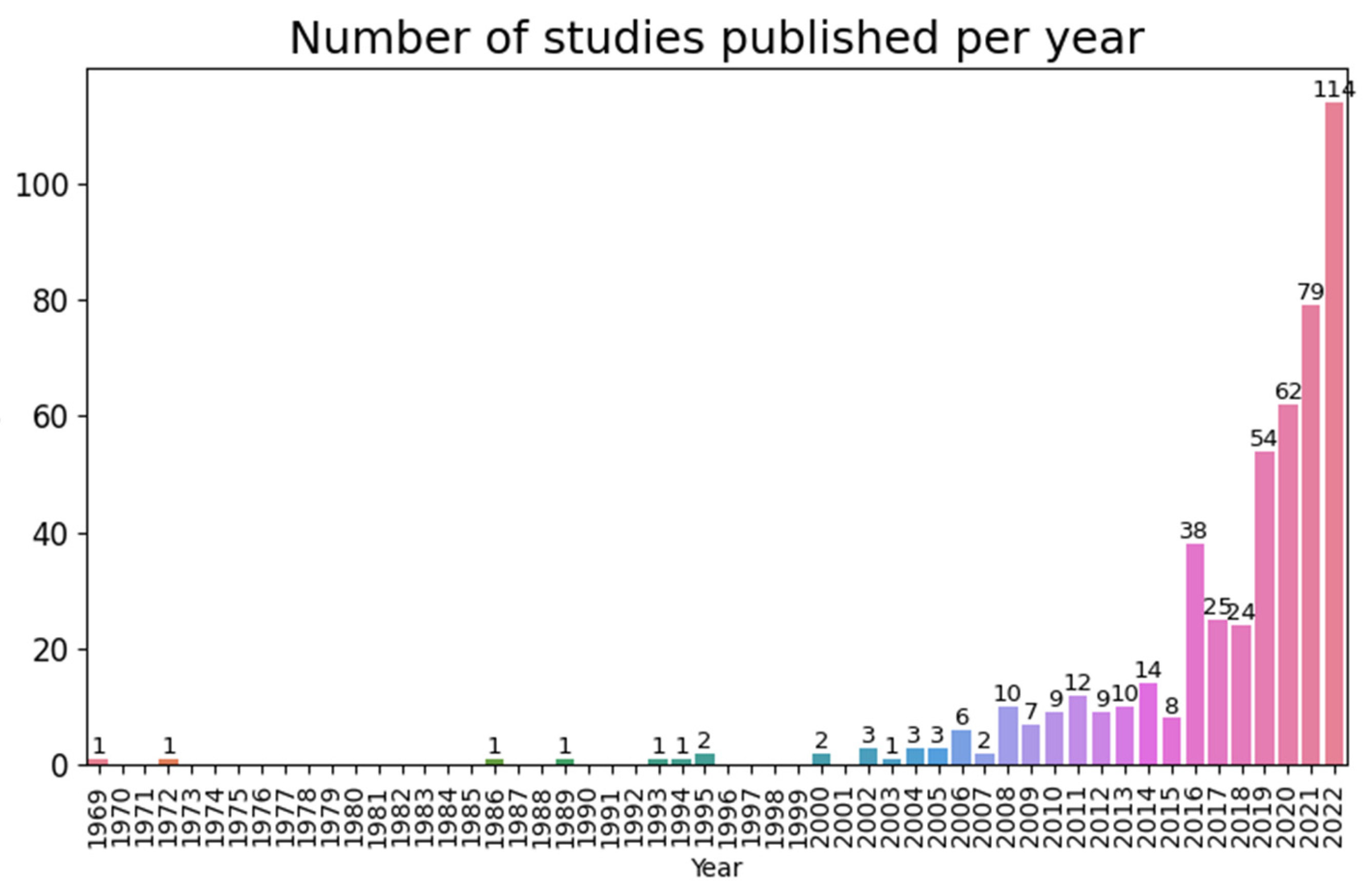
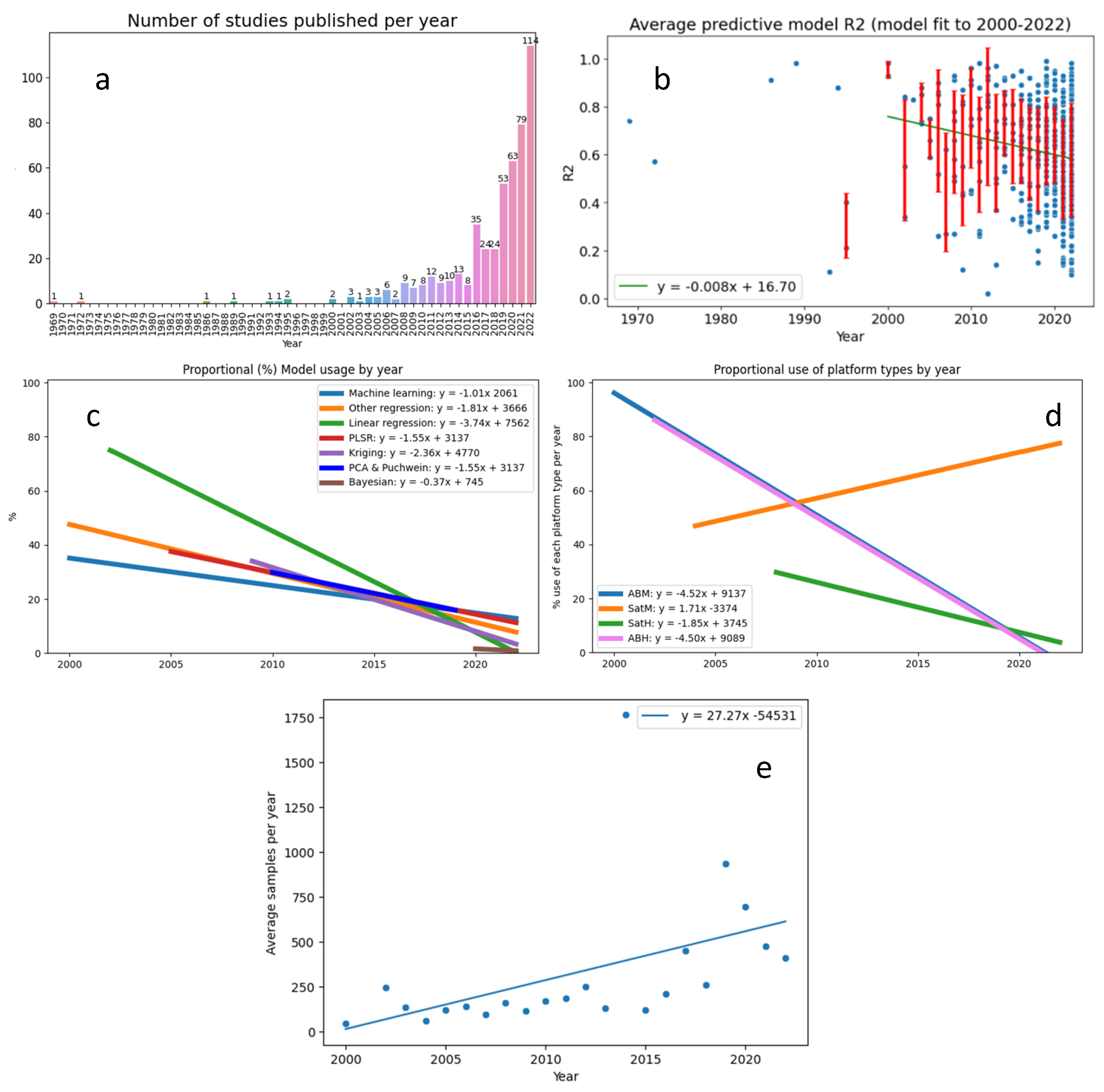
3.1. Publication Record

There has been a sharp increase in the number of soil carbon remote sensing papers published in the past seven years (Figure 1). Prior to 2016, a maximum of 14 soil carbon remote sensing studies was published in a single year (2014). Prior to 2006, there were less than four studies published each year. Though a small legacy of pioneering research published approximately 50 years ago exists, the vast majority of soil carbon remote sensing literature has been published in the past 25 years.

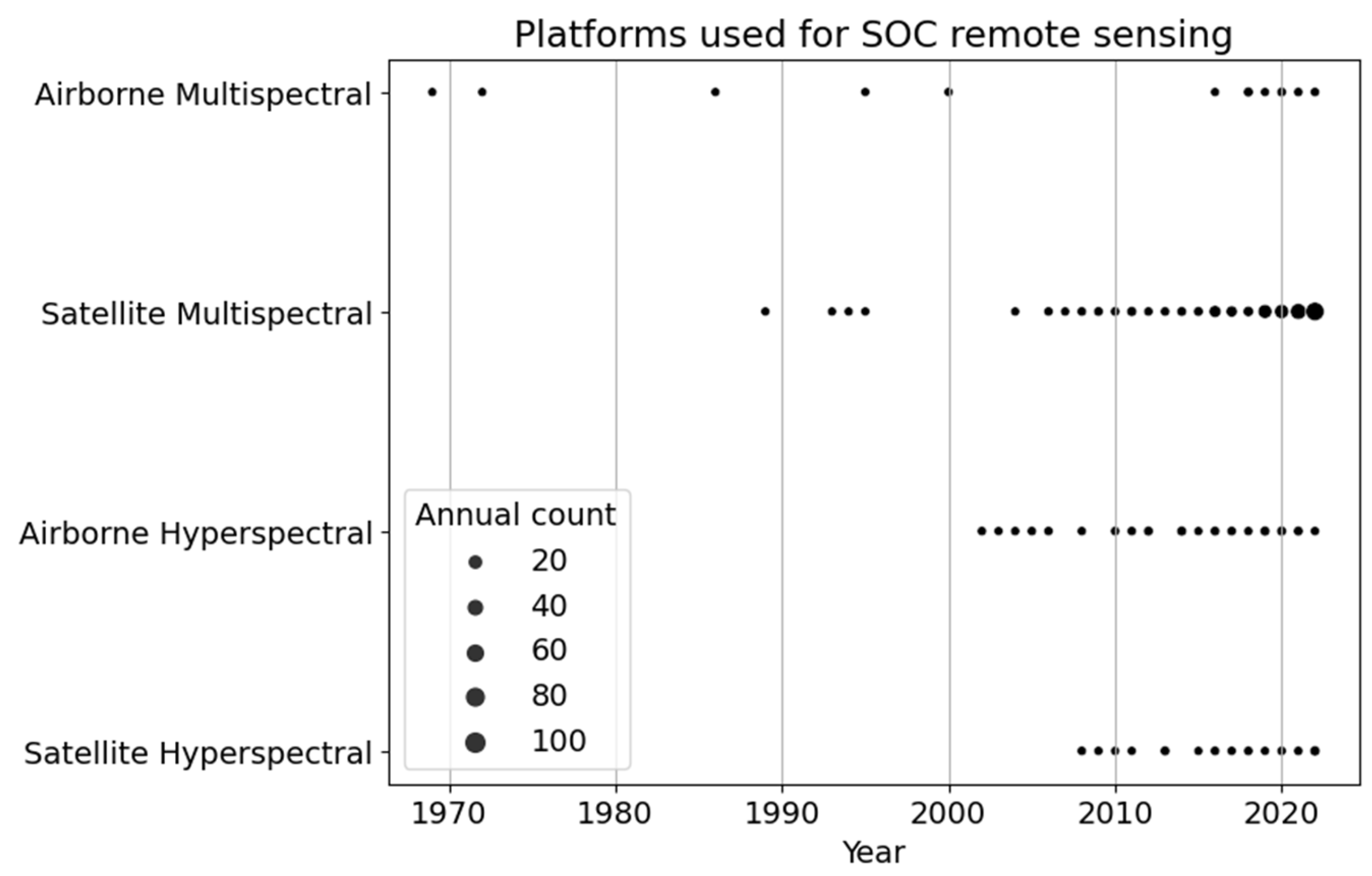
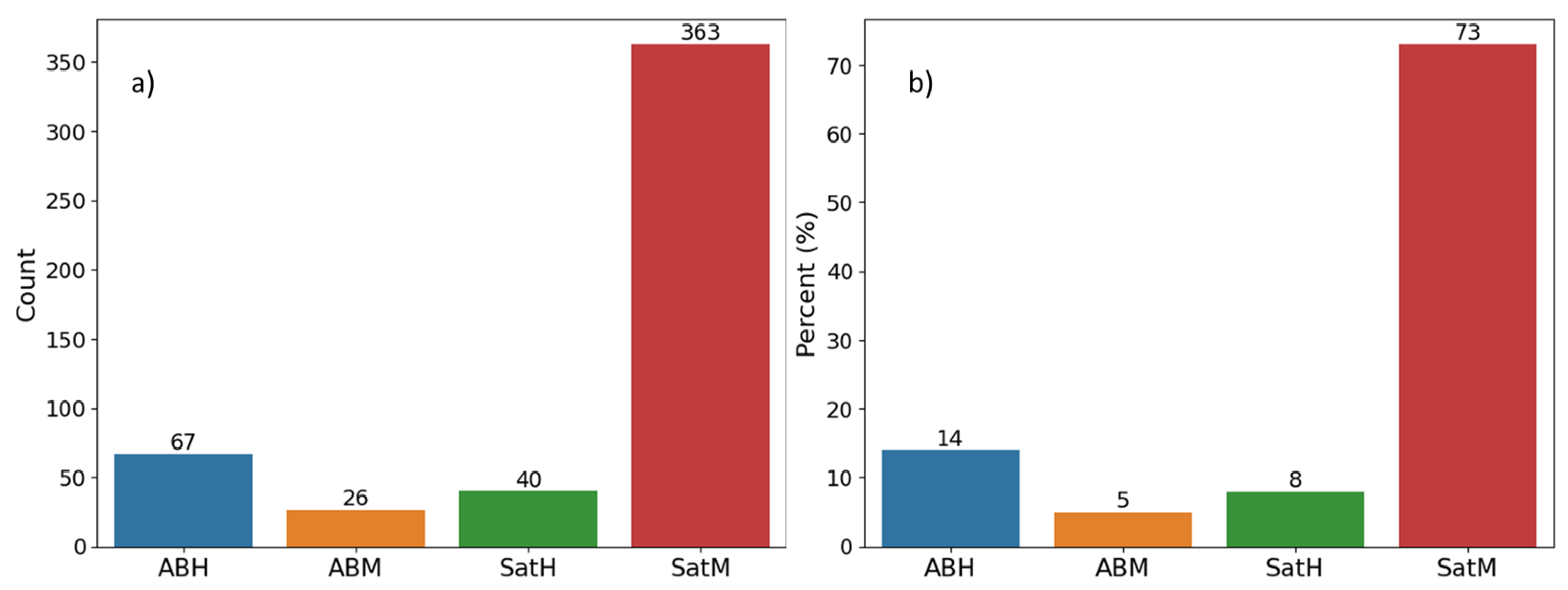
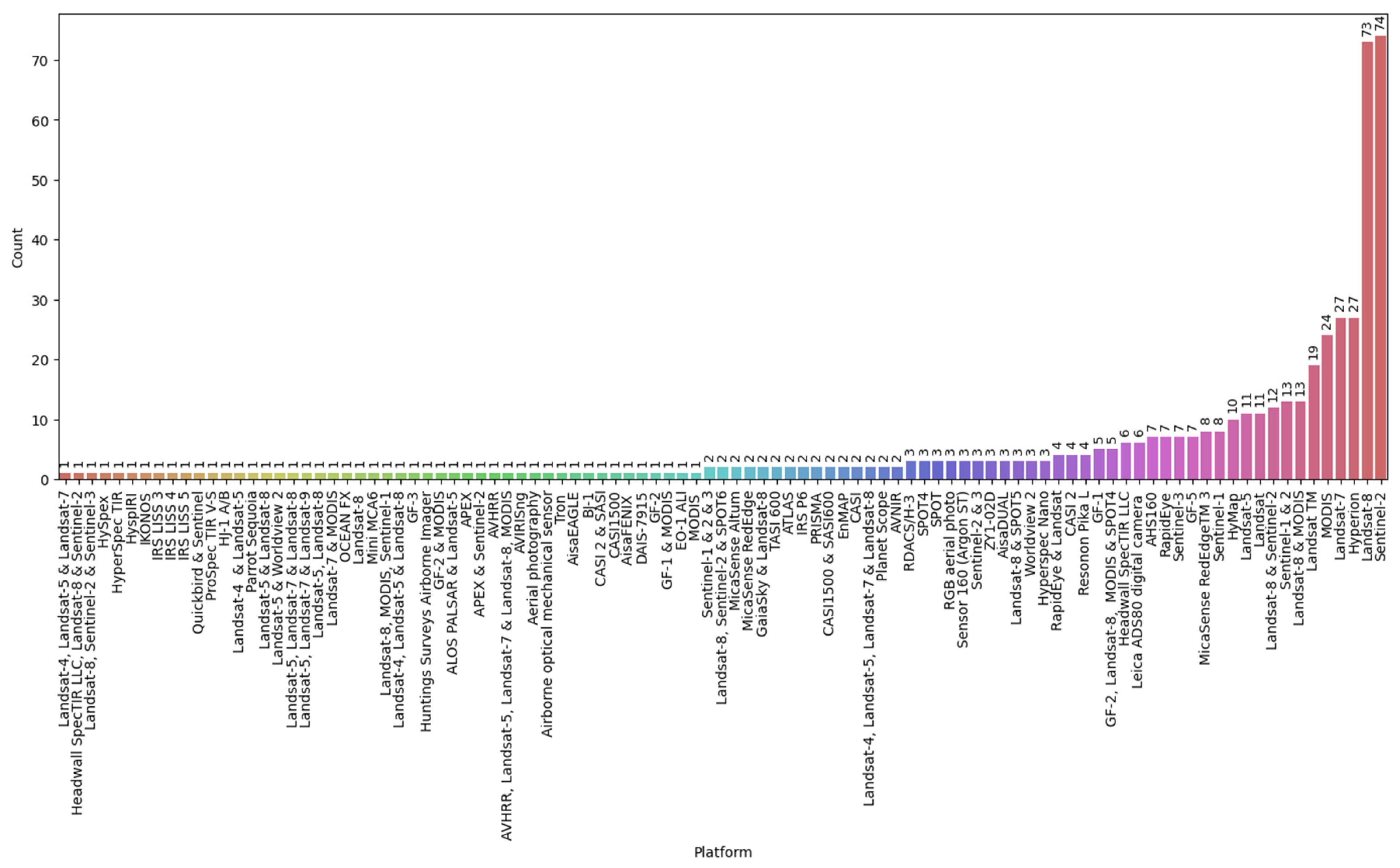
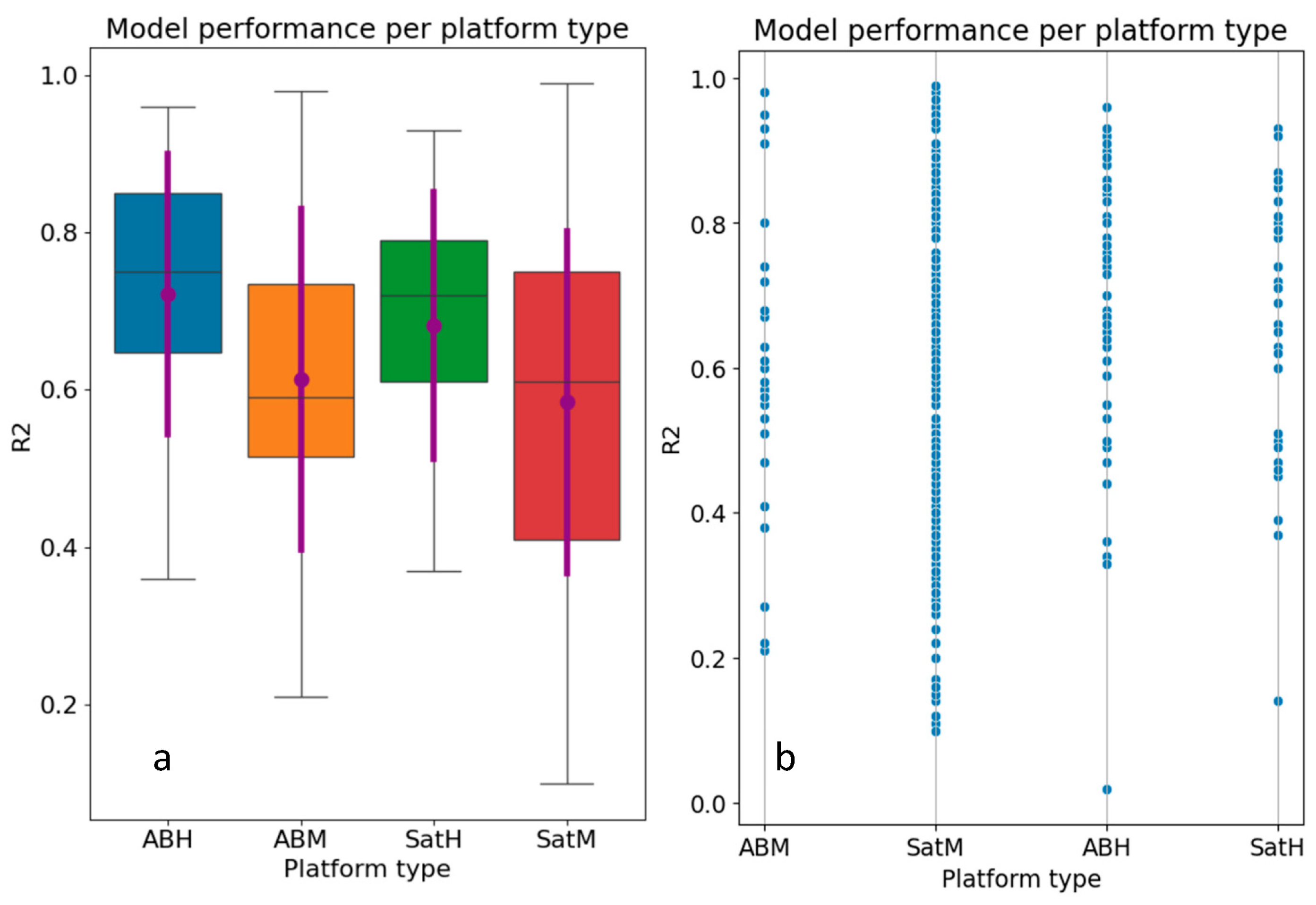
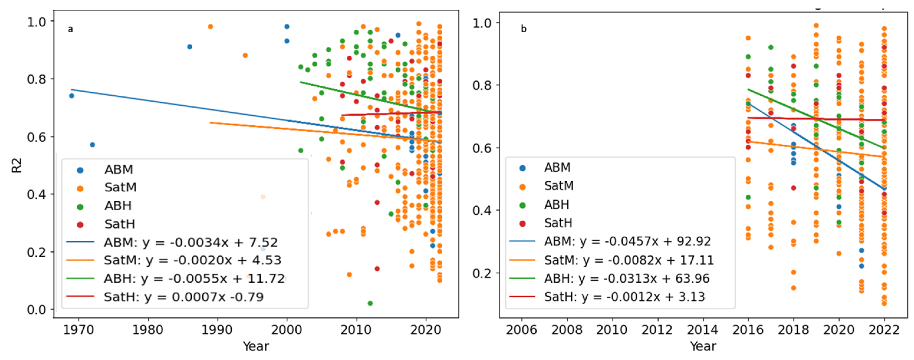
3.2. Platforms and Sensors

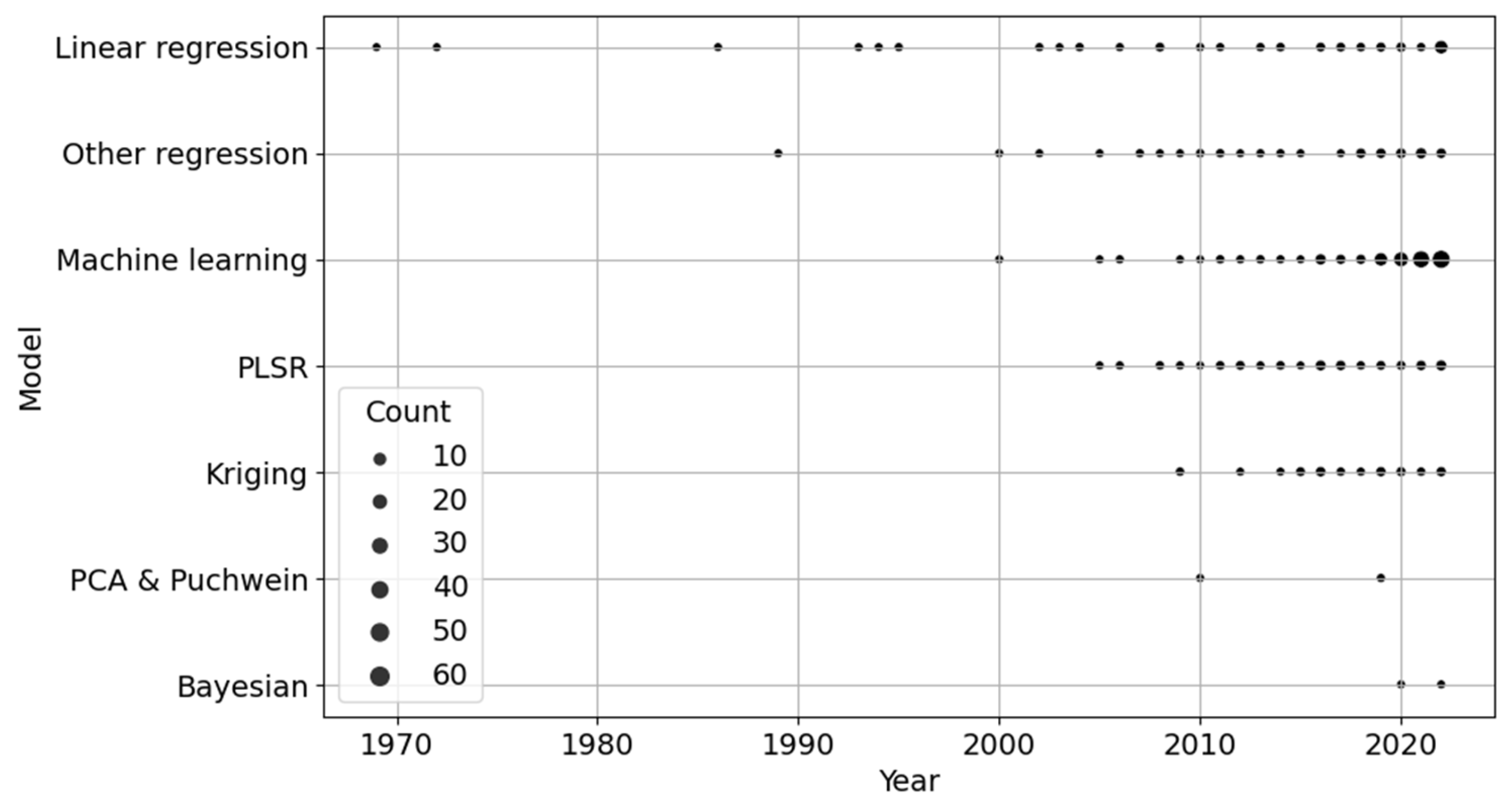
A wide range of platforms and sensors have been used for soil carbon remote sensing. An optical-mechanical scanner mounted on an aeroplane (classified as an airborne multispectral data source) was the first instrument (Figure 2) to be used for soil carbon remote sensing, in 1969 and 1972 [54,55]. Since then, multispectral satellite remote sensing has been used more frequently, with a surge of studies published in the past 5 years. Data from airborne hyperspectral sensors has been used consistently since the early 2000s, while hyperspectral satellite data was not used until the late 2000s.

Multispectral satellite sensors are by far the most common source of remote sensing data (Figure 3a) incorporated in spatial soil carbon prediction models, appearing in 74% of all models (Figure 3b). Airborne hyperspectral (13%) is the next most commonly used, followed by satellite hyperspectral (8%), then airborne multispectral data (6%).

The most commonly utilised remote sensing data applied in soil carbon remote sensing models (Figure 4) is derived from publicly available, free, data sources such as the Landsat and Sentinel satellites. Of all soil carbon remote sensing studies identified, 35% included data from one of the Landsat satellites as a primary data source. Sentinel-2 data were also frequently used. Some studies also incorporated data from multiple platforms. It was most common to combine data from Landsat 8 and Sentinel-2 with data from other platforms, for example, Zeraatpisheh et al. [56], Venter et al. [57] and Garosi et al. [30]. However, numerous data combinations were identified, including the combination of multi-spectral satellite data with hyperspectral UAS data [45].

3.3. Algorithms

Linear regression has been regularly applied in the preparation of soil carbon remote sensing models since the first study [54], published in 1969 (Figure 5). The first use of a non-linear regression model was identified in a study [58] published in 1989, and the first machine learning model (utilising k-means clustering) in 2000 [59]. Other model types such as kriging, Principal Component Analysis (PCA), and Bayesian modelling have only been trialled in more recent years. Linear regression remains one of the most widely utilised modelling algorithms (Figure 5), with 28 soil carbon remote sensing linear regression models published in 2022. However, machine learning algorithms (62 published in 2022) have become increasingly popular.

3.4. Organic Carbon “Types”

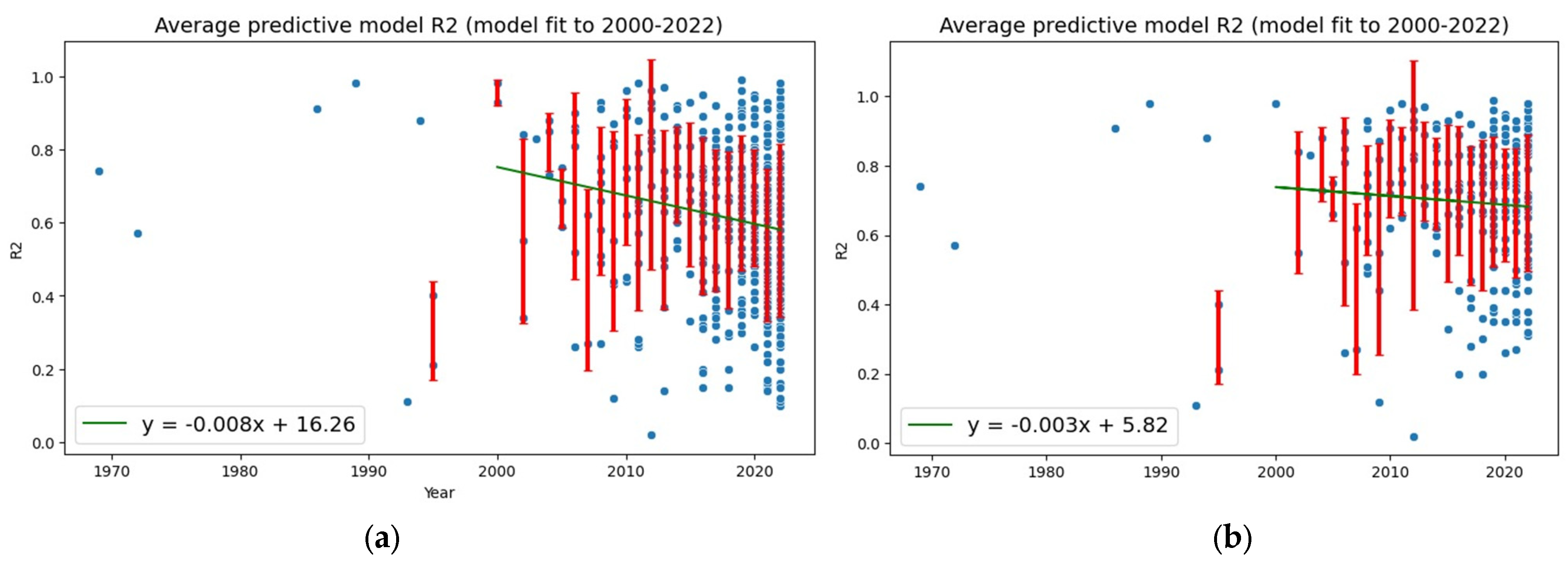
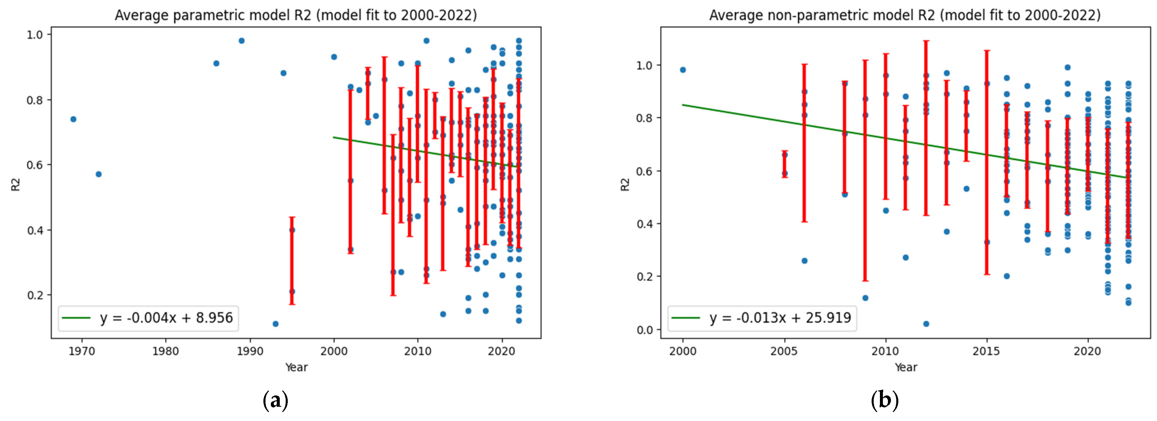
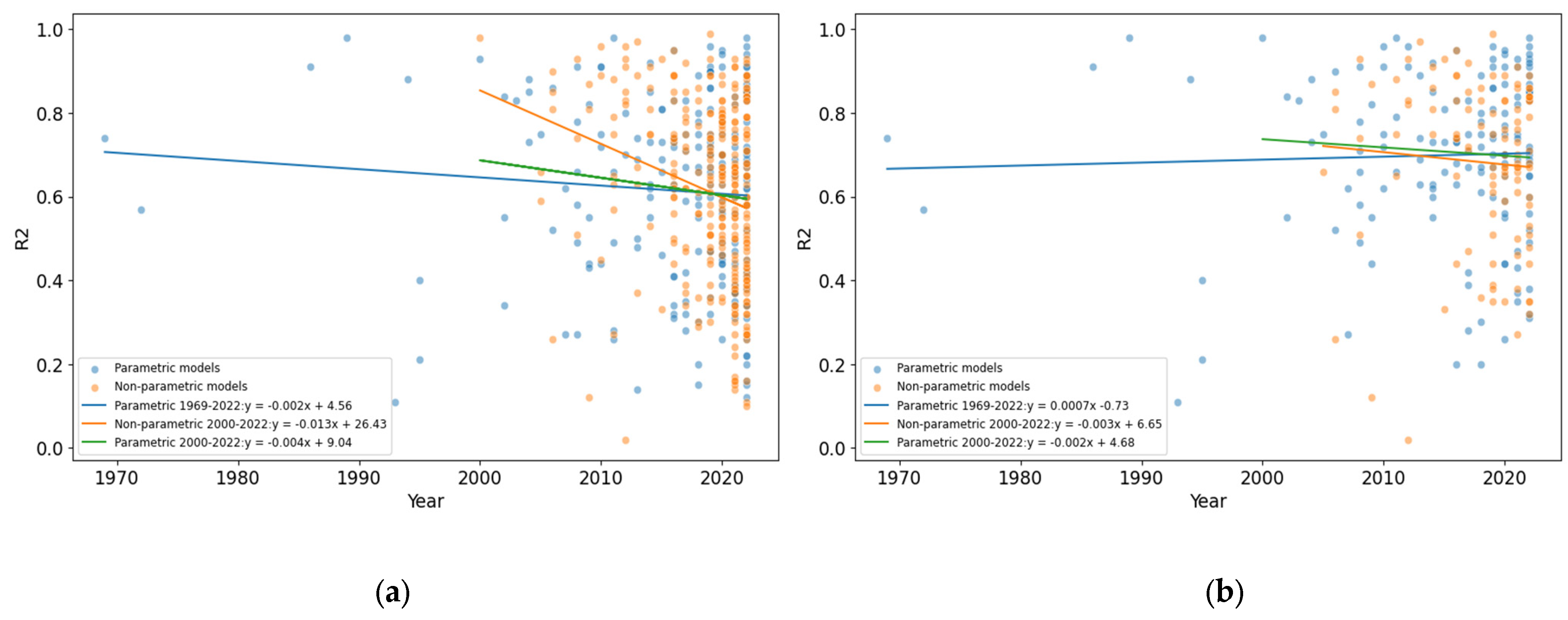
Remote sensing has been used to study a range of organic carbon “types”. Figure 6 shows the eight types of soil carbon referred to in studies included in this review. These are SOCD: Soil Organic Carbon Density; TC: Total Carbon; Carbon; OC: Organic Carbon; Soil Carbon; OM: Organic Matter; SOM: Soil Organic Matter; and SOC: Soil Organic Carbon.

3.5. Performance

Data from a wide range of platforms have been utilised in the preparation of soil carbon remote sensing models. Figure 7 shows the R² of soil carbon prediction models based on remote sensing data from one (Figure 7a) or more (Figure 7b) platforms. It is most common to use data from only one platform; however, there are numerous examples of studies which combine data from a number of sources. Almost all studies which combine data utilise free, publicly available data from multispectral satellites. As an outlier, the only instance identified of airborne hyperspectral data combined with satellite multispectral remote sensing data was presented by Guo et al. [45], who combined data from Sentinel-2, Landsat 8, and the Headwall hyperspectral instrument (Figure 7b).

Overall (Figure 7c), Sentinel-2 and Landsat 8 data are the most commonly used remote sensing data sources for SOC prediction models (note that Figure 7 only includes data sources reported more than five times). The reported accuracy (R²) of soil carbon prediction models is also highly variable (Figure 7a,b). The minimum and maximum reported R² values are, respectively, 0.02 [60] and 0.99 [61]. There is also no obviously “best” data collection platform for utilisation in soil carbon remote sensing models, as evidenced by the wide distribution of model R² values reported for many platforms.

Figure 8a,b show the change in R² for all studies published in each given year since 1969. These figures were generated by plotting the R² value from each published study, then fitting a linear model to identify the overall trend. Figure 8a includes all reported results, including publications which reported the results of multiple studies, or which attempted to construct the reported model in a number of ways. In Figure 8b, only the best model (highest R² for each paper) is included.

Though data are not available for every year (particularly prior to 1990) because SOC remote sensing studies were not published every year, a trend in model performance is apparent. Linear models fitted to the data compiled in this meta-analysis show that, despite a vast increase in the number of studies published, the mean R² of published SOC remote sensing models has not increased with time (Figure 8a), as would likely be expected. This trend is consistent even when only the best model from each paper is included in the dataset considered (Figure 8b).

To assist with interpretation of these negative trends and determine whether the negative relationships are significant, linear models were fitted to the dataset of reported R² results published since the year 2000 (since sufficient data exists from this year onwards). These linear fits are shown in Figure 8 and the uncertainty of the models evaluated with a 95% confidence interval (equivalent to two standard deviations from the mean). The equation of the linear model in Figure 8a is y = −(0.008 ± 0.002)x + 9.78 ± 4.08. The equation of the linear model in Figure 8b is y = −(0.003 ± 0.001)x + 5.28 ± 4.81. These statistics show that the gradient of the linear relationship between model R² and publishing year is negative, even within two standard deviations, even when only the best model presented in each paper is considered. Put another way, there is a very high confidence that the average reported R² of new soil carbon prediction models is decreasing with time.

It is possible that the decrease in the mean model accuracy is related to experimentation with new statistical model methods and approaches, as indicated in Figure 5, especially considering the increasing frequency of novel machine learning model algorithm usage, and the dramatic increase in the number of studies published in 2022 (Figure 1). It was considered possible that the practice of authors providing results from numerous studies in a single paper might have influenced the negative trend shown in Figure 8a. For example, in a single paper, [62] reported the results of nine different soil carbon prediction models (https://data.mendeley.com/datasets/zz4x7xkwkx/1, accessed on 5 February 2023) prepared with the same data and for the same study area, but with different predictive algorithms and arrangements. In the present meta-analysis in Figure 8a, details of all nine reported studies are included. With R² results ranging from 0.45 to 0.7, the lower-scoring models would clearly draw down the average R² for that year (2020) shown in Figure 8a. However, Figure 8b shows the results including only the “best” (meaning highest R²) model–the temporal trend in R² remains negative within uncertainty limits, Accordingly, it is valuable to understand whether differences in the spectral and spatial data resolution, the number of samples used, and the algorithms applied have a significant influence on model R², on average. This information can then be used to inform research and funding priorities in this field.

Since the year 2000, the average R² of non-parametric models has declined much faster than that of parametric models, at an average rate of 1.3% (green line in Figure 9b) per year, in comparison to 0.4% (green line in Figure 9a) per year for parametric models. The equation for the relationship shown in Figure 9a is y = −(0.004 ± 0.002)x + 8.96 ± 5.86. The equation for the relationship shown in Figure 9b is y = −(0.013 ± 0.003)x + 25.92 ± 5.92. These negative gradient relationships are thus statistically significant.

Note the observation that from about 2018, the average reported R² from parametric models is higher than for non-parametric models.

The significant decrease in performance (R²) of both parametric and non-parametric models since 2005 warrants further investigation. Publications demonstrating the use of non-parametric models have increased substantially in number since the first non-parametric soil carbon remote sensing model was published in 2000 [59]. However, the performance of non-parametric models has declined substantially, at an average of 1.3% per year (Figure 9b). This decline is strongly significant statistically. By comparison, the average performance of parametric models has only declined at a rate of 0.2% per year since 1969, or 0.4% per year since 2000 (Figure 10). In recent years, the trendlines in reported model R² have converged and indicate that parametric models (blue line in Figure 10), even when considered over the same time period (green line in Figure 10), are now, on average, performing better than non-parametric models (orange line in Figure 10). The negative relationships shown are significant and are apparent even when considered across other time intervals. For example, the equation for the trendline showing the relationship between reported model R² and year for parametric models published between 1969 and 2022 is y = −(0.002 ± 0.001)x + 4.46 ± 3.82 when all models are included. When only the “best” model from each study is considered, the relationship is y = (0.0007 ± 0.0018)x − 0.73 ± 3.64.

The earliest identified use of a non-parametric model for SOC remote sensing was in a publication by [59]. That study used a minimum-distance/k-means clustering algorithm to predict soil organic carbon/soil organic matter and achieved an exceptional model R² of 0.98. A variety of non-parametric models have been applied since this time, though model performance is declining, on average. Figure 11 demonstrates the declining average performance of four non-assisted model types: Partial Least Squares Regression (PLSR), Artificial Neural Networks (ANNs), Random Forest (RF) and all other Machine Learning models utilised for soil carbon remote sensing model building since their first use in 2005, 2005, 2008, and 2000, respectively.

The categories of other machine learning and PLSR demonstrated the sharpest decline, with y = −(0.025 ± 0.007)x + 51.135 ± 13.207 and y = −(0.013 ± 0.005)x + 26.835 ± 9.790, respectively, while the ANN category (which includes data since 2005) showed the slowest decline, with y = −(0.002 ± 0.007)x + 4.304 ± 14.057. The declining (meaning negative gradient) relationships for the first two of these categories are statistically significant. As for the ANN category, the relationship for the Random Forest category does not have a statistically significant gradient, with the equation being y = −(0.007 ± 0.009)x + 15.467 ± 17.201.

Clearly, none of these categories of prediction model algorithm demonstrate consistently outstanding or improving performance (in terms of R² in SOC prediction models) at this time.

One assumption which is commonly referred to in the relevant literature [25,63] is that increasing the number of samples in a model training dataset will improve the model R². Analysis of the studies in this review’s analysis, however, shows no strong correlation (Figure 12) or statistically significant relationship between model R² and the total number of samples included in the model training, test, and validation data (Figure 12a). This remains consistent even when only models utilising < 400 samples are considered (Figure 12b). Here, the linear models shown in Figure 12a and Figure 12b have gradients of −0.000001 ± 0.000003 and −0.000072 ± 0.000099, respectively, neither of which are statistically significant. Although not shown, restricting the analysis to only the best model per paper does not change the gradients or the results in a statistically significant manner.

It is often assumed that models constructed with hyperspectral data will perform better than prediction models employing multispectral data, and that higher spatial resolution data will improve model performance. Effectively, the use of RGB (visible) or freely available satellite data (e.g., Sentinel or Landsat) is, by some who hold these views, considered a disadvantage. Hence, it is important to clarify the influence of sensor spectral resolution and the spatial resolution of data on model performance, as measured using R². For the following analyses, reported model R² results are separated into one of four categories: Satellite Multispectral (SatM), Satellite Hyperspectral (SatH), Airborne Multispectral (ABM), and Airborne Hyperspectral (ABH), based on the expected spectral and spatial resolution of remote sensing data incorporated into the SOC remote sensing models.

When the effect of the number of samples on model R² is considered separately for each platform type and for different numbers of samples (Figure 13a–d), there is still no strong relationship in most cases. For models constructed with satellite hyperspectral data, there were no significant relationships identified. Statistically significant relationships are as follows: for models prepared with airborne hyperspectral data, there is a marginally significant negative relationship (y = −0.001 ± 0.001)x + 0.75 ± 0.06) in models which used less than 200 samples (Figure 13d) between model R² and the number of samples. For models prepared with airborne multispectral data, there is a negative relationship in all cases (Figure 13a–d). The negative relationship is significant for studies which used less than 5000 and 1000 samples (Figure 13b,c: y = −(0.00081 ± 0.00068)x + 0.72 ± 0.10, and also for studies which used less than 200 samples (Figure 13d: y = −(0.0014 ± 0.0007)x + 0.77 ± 0.10). For models prepared with satellite multispectral data, there is a significant negative relationship between model R² and the number of samples used in studies which include less than 200 samples (Figure 13d; y = −(0.0011 ± 0.00033)x + 0.70 ± 0.04).

When considering the performance of studies from different platform types more generally, Figure 14a demonstrates a slightly higher median R² for studies utilising airborne hyperspectral data (high spectral and spatial resolution) and satellite hyperspectral data (high spectral resolution), but with some outliers, demonstrating very poor model R². Moreover, the standard deviations are very large in all cases: clearly, within the corresponding uncertainty limits, all four platform types have essentially identical performance. Put another way, Figure 14a provides no significant evidence for choosing one of these platform types over another.

Figure 14b clearly shows that a wide range of model R²s are returned from models utilising each data source and that the platform type does not determine model R². A wide range of R² results have been reported for each platform type and, ironically, the highest model R²s were achieved with airborne multispectral (ABM) (lowest spectral resolution), with a maximum R² = 0.98, and satellite multispectral (SatM) data (low spectral and spatial resolution), with a maximum of R² = 0.99.

In summary, the average performance of SOC remote sensing models has not significantly increased through time (Figure 15), even when differences in data resolution (Figure 14) and the number of samples included (Figure 13) are considered. The steepest decline (Figure 15a) in performance is apparent in models utilising airborne hyperspectral data, with y = −(0.0055 ± 0.0037)x + 11.72 ± 7.42. The negative relationship is weakly statistically significant. A weakly statistically significant decline is also apparent for models constructed with airborne multispectral data, with y = −(0.0034 ± 0.0029)x + 7.52 ± 5.81. The negative gradient for satellite multispectral models, y = −(0.0020 ± 0.0024)x + 4.53 ± 4.89, and positive gradient for satellite hyperspectral models, y = (0.0007 ± 0.0059)x − 0.79 ± 0.006 are at best only weakly statistically significant (Figure 15a).

When considered over the recent time period from 2015 to 2022 (Figure 15b), the average performance (R²) of models utilising data from both multispectral and hyperspectral data platforms has declined. Specifically, the relationships in Figure 14b show the steepest decline in average R² from models prepared with airborne hyperspectral data, with y = (−0.0313 ± 0.0122)x + 63.96 ± 24.69. Other significant declines are apparent for models constructed with airborne multispectral data (y = −(0.046 ± 0.025)x + 92.92 ± 49.38) and satellite multispectral data (y = −(0.0082 ± 0.0062)x +17.11 ± 4.11). The relationship for models constructed with satellite hyperspectral data (y = −(0.0012 ± 0.0128)x + 3.13 ± 25.88) does not have a statistically significant sign for the gradient within two standard deviations.

Most of the significant relationships between model R² and other variables considered in this study have negative temporal gradients. In most cases, these results are counter-intuitive in that progress is expected to yield positive temporal gradients; accordingly, they warrant more detailed investigation and should be the subject of future studies.

In the meantime, this meta-analysis highlights the need to re-evaluate some common assumptions and research priorities in the industry. Specifically, the requirement for high spectral and spatial resolution data, and the associated computing capacity for data processing, should not be overestimated. Basic SOC prediction models incorporating less than 200 samples, constructed with low spectral and spatial resolution data, can perform well and return high performance (R²) metrics.

4. Discussion

This review analyses the long tradition (50+ years) of attempts at soil carbon remote sensing. Some of these attempts yielded higher accuracy than others. The first two soil carbon remote sensing studies, published in 1969 [54] and 1972 [55], utilised very basic equipment, prediction algorithms, and computing power. This is a stark contrast to some studies published in recent years, which utilise the latest sensors, vast amounts of data (spectral and spatial layers) and computing power, complex models, and state-of-the-art machine learning algorithms. Surprisingly, the vast improvements in data processors, the spectral and spatial resolution of sensors, and the availability of remote sensing data have not led to significant improvements in the performance of soil carbon prediction models. In fact, the performance of soil carbon remote sensing models has been declining through time (Figure 8, Figure 9, Figure 10 and Figure 11).

Other reviews of soil carbon remote sensing [15,18,20,23] and digital soil mapping [24] studies appear to have not included early papers on these topics. Some reviewers have even mentioned an absence of relevant papers published prior to 2000 [18] or only one UAS study published prior to 2019 [64]. This is unfortunate, as there appear to be lessons to be learned from the basic, low-tech approaches applied in early studies. The solid performance with R² = 0.57 to 0.98 [54,55,58,65] demonstrated pre-1990, utilising basic instrumentation, data processing algorithms, and technology presents a good starting point for discussion of the optimal spatial resolution, spectral resolution, and best wavelengths for effective SOC remote sensing. It is also recommended that future authors of soil carbon remote sensing studies interact with these early publications, to allow a more informed decision of necessary instrumentation, computing power, and expertise [24], especially in budget- and resource-limited research environments [66].

4.1. Model Training Data (Number, Density, and Distribution of Samples)

Figure 12 and Figure 13 show that there is not a strong positive relationship between the number of samples included in a model and the resulting model R², when these two variables are considered independent from other factors. However, the size of the study area and the resulting sample density seem likely to influence these relationships and should be considered in future studies, when possible.

The size of the study areas included in this meta-analysis were highly variable, with some studies considering only one or two fields [55] and others considering large areas, like the entirety of Scotland [67]. Though 197 samples were included in the former study and 27,833 samples included in the latter, the former had a higher sampling density due to the smaller study area size. Analysis of the effect of sample density could not be undertaken in this review, however, as many studies did not clearly specify the size of the study area. In addition, not all studies detailed the number of samples included in model building, and many studies did not detail how sample populations were divided between training and test datasets. Hence, differences in sample density may be an explanatory factor in the trends presented, but we were unable to consider the influence of this variable in this meta-analysis due to an absence of reliable information on this topic.

Despite this result, some studies still report the number of samples as a limitation on model performance [68]. Other studies include evidence to support this point. For example, Touré & Tychon [69] demonstrate a minor improvement in model R² from 0.85 to 0.88 when increasing the number of model training samples from 68 to 77, for a model constructed with CASI 2 hyperspectral data and a Stepwise Multiple Linear Regression algorithm. In a study utilising aerial photography to map SOC across a 115 ha agricultural field in Georgia, USA, [59] found that the RGB image-derived SOC prediction model R² could be improved from 0.93 (28 samples) to 0.97 with the inclusion of an additional 31 samples. In both of these examples, modest improvements in model performance were achieved by increasing the number of samples included in model training datasets.

The density of sampling across a study area is another way to consider the effects of sample numbers on model performance. There is apparently evidence to indicate that sampling density has a significant impact on the performance of some prediction algorithms, particularly those utilising Kriging approaches [70,71]. However, the influence of sample density on the performance of machine learning models is less well understood [72]. Some studies have addressed this topic. For example, [47] recommends the use of a Support Vector Machine algorithm over Random Forest in scenarios when few model training samples are available. Unfortunately, sampling density could not be calculated and reported for studies included in this meta-analysis, as the size of the study area, and details of the segmentation of samples between model training and test regions, were often not reported clearly. In some publications, the number of samples utilised was not reported at all.

Soil inhomogeneity exists on a range of temporal and spatial scales [73], and, therefore, soil sampling design may also influence the performance of a soil prediction model [74,75]. Though not considered in this meta-analysis, [74] demonstrates the importance of soil sampling design on SOC prediction model accuracy. In that study, two different sampling strategies were employed and compared for their effects on the resulting model predictive capacity. The model constructed with samples collected in a grid pattern (R² = 0.45) exceeded that of the model constructed with randomly selected (R² = 0.27) sampling points.

Sampling regimes are an important consideration for soil property modelling, as they may introduce bias to the model if a representative range of samples are not collected [75]. Ideal sampling strategies will cover spatial and (if relevant) temporal variability across the study area. It is noted that a number of studies reviewed in this meta-analysis reported testing and correction for a number of bias types, including negative [76], validation [77], and prediction [78] bias.

Apparently, Digital Soil Models (DSMs) often do not perform as well as soil carbon remote sensing models [68,79]. Soil properties change over time, influenced by land management, soil amendments, climate, and other environmental conditions [73,80]. Hence, the temporal variability of soil properties [81] may explain why DSM and other approaches utilising historical or legacy data [24] often do not perform to the same standard as other SOC modelling approaches which incorporate multi-temporal data or up-to-date environmental, terrain, soil, and climatic data [82]. The use of historical data means that the spatial distribution of samples cannot be controlled without subsampling the dataset [24]. Sampling and image acquisition dates also cannot necessarily be aligned, resulting in the modelling of soil properties with imagery from a different time period. It is expected that legacy data introduces error to soil carbon prediction models if it is not matched to remote sensing data from the same time period.

The carbon or organic matter content (%) of the model training samples can also influence model prediction accuracy. For example, Lin et al. [83] found that prediction accuracy improved substantially between areas where SOM was greater than 24g/kg (R² = 0.75) compared to R² = 0.35 in other areas. In an Uncrewed Aerial System (UAS) soil carbon mapping exercise at the Hoosfield Spring Barley experiment in Harpenden (Rothamsted, UK), Aldana-Jague et al. [84] identified consistent bias in the Support Vector Machine model utilised, where the model underpredicted SOC stocks in areas with >3% SOC and overestimated in areas of <3% SOC. This was attributed to skewed population of SOC data points in the model training dataset. Thus, future studies could explore the influence of the distribution and range of soil carbon values for soil samples (e.g., 1–2% SOC compared to 1–6% SOC) on model R², and therefore, whether this analysis should be considered as a multi-variate problem.

In addition, other possible lines of exploration include the influence of sample density on model R² and the trends observed in model performance when additional or alternative statistical measures of model performance (e.g., reduced chi square, RMSE, ME) are used.

4.2. Best Wavelengths

This meta-analysis did not collect data on the wavelengths and bands utilised in each SOC prediction model specifically; however, the spectral range and resolution of sensors mounted on each platform is known, allowing for indirect determination of the wavelengths and bands. A number of authors reported trials of soil carbon prediction over an area with remote sensing data from different sensors [7,19,85]. A number of other studies reported a trial-and-error approach for selection of the best wavelength/band combinations [54,59,86]. It is also noted that most model training algorithms use an iterative approach, subsampling data from different wavelengths or bands, to identify the best wavelength combination [87]. This is usually undertaken without specific intervention by the user, beyond the selection of the number of preferred variables.

Previous literature identifies strong correlations between RGB bands in terms of SOC prediction [88], suggesting redundancy in the RGB bands and decreased model performance when RGB bands are utilised [89]. However, a number of studies identified in this meta-analysis demonstrated exceptional model performance utilising only RGB wavelengths, for example, [54].

Žížala et al. [53] compare the performance of resampled data from five satellite and airborne remote sensing platforms for SOC prediction over a 1.45 km² agricultural plot in the Czech Republic at 1 m resolution. In this study, the Parrot Sequoia and Parrot Disco Pro sensors (used together) mounted on a fixed-wind UAS demonstrated comparable calibration model performance (R² = 0.72) to Sentinel-2 (R² = 0.72) and PlanetScope (R² = 0.75) models, and considerably better performance than the Landsat 8 model (R² = 0.45). These findings should not be taken out of context, however, as the SOC prediction model (R² = 0.72) prepared with one-metre resolution Parrot Sequioa data performs worse (R² = 0.52) at ten-metre resolution. Therefore, it appears that remote data resolution was more significant than the wavelength bands and sensors used in this case.

It should also be noted that numerous spectral indexes used in SOC prediction models rely solely on RGB data, including NBAR2 (Normalised Burn Ratio 2), NGRDI (Normalised Green Red Difference Index) [89], redness index [81], and coloration index [90]. Hence, there is extensive published literature with which to test the nuances of the claim of RGB data, causing model redundancies in future analyses and reviews. One consideration in the use of RGB spectral indexes is the likely spectral interference from the weathering of clay minerals [91,92]. In arid and desert environments, or other areas with extensive soil weathering, weathering of iron and clay minerals is common. Hence, the presence of weathered soils may reduce the precision of models generated with spectral data or indices utilising RGB/visible (especially red) wavelengths [45].

Though vulnerable to some environmental variables (soil moisture, weathered clay minerals, etc.), it is clear that RGB data have potential in soil carbon predictive modelling applications. Therefore, it should not be immediately ruled out as a data source, even where concerns regarding multi-collinearity and potential redundancy exist.

4.3. Best Algorithm

It is apparent that there is no consensus on the “best” algorithm to apply to soil carbon remote sensing models. Results from this meta-analysis do not indicate a clear winner in terms of model performance (Figure 10 and Figure 11). Multiple publications apply a range of algorithms [45,93] to the same training datasets in an attempt to identify the “best” modelling algorithms, combinations of variables, and data resolution. It is clear from relevant literature that testing, comparison, and evaluation of the “best” algorithms, scales, and variable combinations is ongoing, as little consistency is apparent between the results presented.

Though linear regression is the most commonly applied algorithm in soil carbon prediction models, the use of machine learning and other algorithms has increased rapidly since 2000. In 2022, ANNs and other machine learning algorithms were the most common type of algorithms applied in soil carbon remote sensing models (Figure 11). There are many different types of machine learning models, and most include several hyperparameters (parameters which are set prior to the initiation of the learning process) which must be set by the user [68]. For example, an RF algorithm requires the user to define (a) the number of observations in each tree, (b) the number of variables randomly drawn for each split, and (c) the minimum number of samples in each node [94]. These parameters may be tuned manually, or with optimisation techniques [95,96].

4.4. Effects of Spectral Resolution—Is Hyperspectral Better than Multispectral Data?

It is commonly assumed that soil carbon models incorporating hyperspectral remote sensing data will perform better than models incorporating multispectral data [64]. Improved performance has been demonstrated in a number of studies. However, this is not true in all cases, or on average. For example, Castaldi, Chabrillat [61] demonstrated a multispectral satellite SOC prediction model outperforming a hyperspectral satellite data-based model across temperate croplands near Demmin, in northeastern Germany. However, in this review, aggregated results demonstrated that models incorporating hyperspectral data were not intrinsically more accurate than models generated with multispectral data (Figure 14a,b).

A study by Žížala, Minařík [53] compared the ability of three machine learning models for their SOC predictive ability when trained on a range of datasets from multispectral and hyperspectral sensors. Models generated with multispectral data from Sentinel-2, Landsat 8, PlanetScope, and a Parrot Sequoia sensor were compared to models generated with hyperspectral data from the CASI1500 and SASI600 sensors mounted on a UAS. Despite relatively high spatial resolution in some of the multispectral datasets, the hyperspectral UAS (highest spectral range and resolution) data consistently produced a better predictive model than models generated with multispectral data. In that case, it should be noted that the hyperspectral sensors (102 bands) had an order of magnitude more spectral bands (and so, data) than the multispectral sensors (4–10 bands).

Guo et al. [45] generated a soil carbon prediction model with remote sensing data from three sources and found that the model generated with (airborne) Headwall–Hyperspec instrument data returned a substantially higher R² = 0.72 than models generated with Sentinel-2 (R² = 0.42) or Landsat 8 (R² = 0.26) multispectral data. Both the multi-versus hyper-spectral nature of the data and the spatial resolution (airborne versus satellite) of the data are thus different.

Similarly, Biney et al. [97] compared the performance of hyperspectral UAS and multispectral Sentinel-2 data for SOC prediction across an area of 22 ha of agricultural fields in the Czech Republic. They presented improved model R² results for the soil carbon prediction model generated with hyperspectral data (R² = 0.27) compared to the model generated with multispectral data (R² = 0.15). However, the model R² presented was low under all scenarios for that study, and the influence of spectral resolution was not differentiated from the possible influence of different spatial resolutions.

Mzid et al. [19] compared the performance of soil carbon prediction models generated with data of the same spatial resolution from PRISMA, Sentinel-2, and Landsat 8 data. In this case, it was also found that the soil carbon prediction model generated with hyperspectral data (R² = 0.85) performed better than the models generated with Sentinel-2 (R² = 0.68) and Landsat 8 (R² = 0.60) multispectral data. Again, the effects of both spectral and spatial resolution need consideration.

Based on the results of Mzid et al. [19], it appears that models generated with hyperspectral data should perform better, when all other factors are equal. However, results from this review showed that the best-performing studies utilise airborne multispectral or satellite multispectral data (Figure 13). Some insight into these contrasting results may be provided by the results of Castaldi, Hueni [98], who considered the importance of spectral and spatial resolution on SOC predictive model performance by reusing and resampling data at various resolutions. It was found that resampling hyperspectral data to Sentinel-2 wavelengths (thereby reducing the spectral resolution) did not diminish model performance at most (4 of 5) sites. Instead, differences in model performance could be attributed to spatial resolution and signal-to-noise ratio of the data. Hence, future analyses and reviews could compile quantitative data regarding spatial resolution (e.g., 1 m, 10 m, 100 m) and signal-to-noise ratio (SNR) to determine the relative influence of each of these factors on model R².

Another interpretation of the disparity between the aggregated results presented in this review and individual model results presented in studies comparing models prepared with high and low resolution data is that other differences in the use of ancillary (terrain, climate, geological) data directly influence model performance (R²). Commonly, soil carbon models utilising hyperspectral data avoid incorporating additional geographic and climatic data due to the already-existing high-dimensionality of the modelling dataset. It has been suggested that this practice (of excluding data regarding other variables) impacts the accuracy of soil carbon prediction models utilising hyperspectral data [86]. Future reviews could consider the influence of environmental and climatic variables on soil carbon model performance and clarify the relative importance of ancillary data in comparison to the spatial and spectral resolution of remotely sensed data.

Nevertheless, the soil carbon prediction model results summarised in this review clearly demonstrate that the use of large volumes of data or high spectral resolution data does not guarantee robust model performance (Figure 14).

4.5. Model Bias

Model bias may be defined as the presence of systematic error in a model which results in the model making consistently incorrect predictions [99]. Many types of bias exist, including confirmation bias, sampling bias, coverage bias, and reporting bias [100]. It is typical during the construction and testing of remote sensing models to assume that model-based predictors will exist without bias [101]. However, model-based predictors can be a major source of bias in remote sensing models [102] where the real values deviate strongly from the mean [103], meaning there is a large residual. In such situations, by trending towards the mean, the model will over-predict the proportion of values close to the mean and under-predict the proportion of extreme values [101,102]. It appears to be possible to reduce offset model bias in remote sensing models using classical calibration approaches developed in the field of chemistry [101]; however, applying such offsets or corrections appears to be an uncommon practice.

In an evaluation of error sources in SOC remote sensing models, Goodwin et al. [6] found, based on a Student t-test, that models incorporating only reflectance data incorporating remote sensing data, digital soil maps, and soil reflectance data collected with a handheld spectrometer. This was consistent with the findings of Wang et al. [104], who found that segmenting modelled areas according to soil type reduced model bias. In some other recent studies [23,105], model bias was not directly measured or addressed. Instead, authors relied upon bootstrapping [106] or model algorithms which use cross-validation to manage model bias [8,107,108]. When bias was measured directly, mean error [109], a specified bias equation [91], and the Horvitz–Thompson (HT) estimator [110] were some of the metrics used.

4.6. Bare Soil Masking

Bare soil masking has previously been identified as a common and important step in the preparation of spatial models predicting soil properties [23]. Bare soil masking also appears to improve the performance of soil carbon prediction models [111], and studies employing a bare soil mask typically report a solid soil carbon predictive model performance [112]. For example, Dvorakova, Heiden [113] reported that the refinement of the bare soil mask was critical for bringing the performance of their SOC prediction model up to an acceptable level (R² of 0.54, improved from R² of 0.3). Comparing SOM model performance on MODIS images from three dates, multiple years apart, Dou et al. [114] found that the model performed better when applied to images of fields with less crop residue (equivalent to greater bare soil area).

Bare soil masks are regularly based on NDVI thresholds, with threshold values set to values in the ranges of 0.35–0.20 [23] or 0.22–0.10 [115] defining different land cover classes. A Normalised Burn Ratio 2 (NBR2) index of 0.05 [116], or other similar value, could also be used. The latter is particularly useful in identifying bare soil pixels where crop residue is present. Other NBR2 thresholds were trialled by Castaldi et al. [116]; however, these returned worse model accuracy results (R² of 0.84 and 0.31 for thresholds of 0.075 and 0.1, compared to 0.94 for the 0.05 NBR2 threshold).

In Australia, opportunities for soil carbon remote sensing could be improved through the generation of bare soil composites such as those presented by Safanelli et al. [117], to allow bare soil areas to be readily identified and targeted for fieldwork and SOC remote sensing studies.

4.7. Influence of Soil MC on SOC Remote Sensing Model Performance

It is claimed that soil moisture is the primary limiting factor in monitoring soil attributes with hyperspectral technology [4] and the largest source of error in SOC spectral prediction models [118]. Weight is added to this argument by a number of studies [76,119,120] which demonstrate improved soil carbon prediction from dry soil, especially in bare soil regions. This improvement in model performance is likely due to the high correlation between SOC and soil moisture in the visible, NIR, and SWIR bands [10,121,122].

Radiative similarities between soil carbon and soil moisture are sufficiently strong that SMAP (Soil Moisture Active Passive) SAR (Synthetic Aperture Radar) data products have been used for soil carbon prediction modelling [76]. In some cases, the soil moisture content has even been used to infer soil carbon stocks with reasonable accuracy [36], meaning R² = 0.7.

4.8. Influence of Soil Type

Zhang et al. [10] demonstrate the influence of soil type on SOM predictive model performance, with one SOM prediction model applied to two “typical” cropland sites with different soil types returning different results. The prediction model applied to an area of Phaeozem soils returned an R² and RMSE of 0.75 and 0.79, respectively, while the same model returned an R² and RMSE of 0.65 and 0.55, respectively, when applied to an area with Arenosol soils. Thus, it appears as though soil type can be an important quantity in determine SOC levels, not surprising intuitively.

4.9. Measurement Technique for Calibration/Model Training Data

A range of laboratory-standard soil carbon measurement techniques exist [16]. In an SOM remote sensing study in Nepal, Lamichhane et al. [123] applied a correction factor of 1.3 to all laboratory SOM measurements to account for partial oxidation of the organic matter. This is an unusual practice in soil carbon remote sensing studies. However, the effects of sample handling, preparation, and pre-treatment on the degradation of SOM and SOC are well documented [124,125,126], even if not well known. Where soil carbon data from a range of sources is integrated or absolute values of stored carbon (for example in the calculation of carbon stock for carbon credits) are of interest, it is likely important to consider the effects of sample handling, preparation, and pre-treatment on carbon stored in soil samples.

4.10. Model Accuracy Metrics

Though some may suggest that other model performance metrics such as RMSE are more appropriate, R² was chosen in this review, as it was the most widely reported statistic. RMSE statistics were also recorded, when available. Various authors argue that RMSE is a problematic metric for comparing studies where there is a variable range or skewed distribution of SOC or SOM in each study area, as the magnitude of error is proportional to the range of SOC across the study area [23]. Instead, a proportional metric is suggested for the quantification of error [23].

For example, in some studies, the SOC content of samples across the study site ranged from 0.01–70.8% [67], while in the Nile Delta of Egypt [127], the range of SOC values recorded from samples collected across the study area was only 0.04–1.57%. Correspondingly, the reported RMSE of SOC predictive models was 8.1% and 0.02%, respectively, for these two studies. It is expected that the large difference in RMSE for the Aitkenhead and Coull [67] study is due to the difference in SOC stocks across the study area, and not representative of the difference in the model’s predictive capacity.

RMSE was also problematic to record and compare, as it was reported in many different ways. Some studies reported RMSE as a percentage, others in g/ha or g/100 g⁻¹, and others as a normalised RMSE value. Differences between reported units add additional complexity to the aggregation and interpretation of these model error metrics, and hence, they were avoided.

4.11. Overall Summary of Findings

It is usually the case that performance and insights improve through time as a discipline matures. However, in the case of soil carbon remote sensing, the average model performance is statistically declining with time for data of all spatial and spectral resolutions (Figure 8, Figure 9, Figure 10, Figure 11, Figure 14 and Figure 15). The steepest declines in model performance are apparent in models utilising airborne hyperspectral data (Figure 15a). However, the performance of models utilising airborne multispectral and satellite multispectral data, and to a lesser extent airborne hyperspectral data, are also dropping (Figure 14b). These results are unexpected and suggest that the influence of systematic changes in model assumptions, planning, preparation, or testing is to blame. Since time appears to be the explanatory variable, Figure 16 is presented to stimulate future discussion regarding the drivers of this decline in model R².

Figure 16b demonstrates that the R² of published models has, on average, declined through time, and more consistently since 2000. The decreasing average model R² coincides with a substantial increase (Figure 16a) in the number of studies published since this time. Proportionally, there has been an increase in the use of satellite multispectral data (Figure 16d) and machine learning algorithms (Figure 16c) applied in soil carbon remote sensing models. The number of samples utilised (Figure 16e) has also increased on average.

As multispectral satellite data (utilised by a majority of recent papers) becomes increasingly available through platforms (such as Google Earth Engine) offering free, pre-processed data, online processing capability, and numerous other features, it could be expected that the use of such data (multispectral satellite) would increase, compared to data from other platforms (such as costly airborne hyperspectral data). This is consistent with results from the studies compiled (Figure 16d). The increased use of satellite multispectral data, cannot, however, be used to explain the average decrease in average annual model R² since Figure 13b demonstrates that some models utilising satellite multispectral data perform exceptionally well, and hence, the use of such data should not be considered an intrinsic disadvantage.

An increase in the average number of samples utilised (Figure 16e) also appears unlikely to reduce the average model R². Hence, the negative correlation between model R² and use of machine learning (Figure 16c) and non-parametric (Figure 9b and Figure 10) models may provide insights into recent trends.

Figure 16c demonstrates a surge in the proportional use of machine learning algorithms in recent years. A simple interpretation of this relationship could be that machine learning is poorly suited, or not yet being applied appropriately, to soil carbon remote sensing challenges. However, exploratory analysis and experimentation with new model algorithms, assumptions, and approaches is a valuable activity, and in most situations, extensive experimentation is required for long-term improvement. In this case, it seems possible that increased experimentation and publication has recently lowered expectations for model performance, leading to a decrease in average annual soil carbon remote sensing model R².

Assuming this is the case, it appears that much more experimentation and work is required to determine the usefulness and appropriateness of machine learning and other non-parametric algorithms in soil carbon remote sensing modelling exercises. As machine learning algorithms typically require vast amounts of training data, a strong focus must be placed on making soil databases and other data repositories publicly available. In turn, this may require a re-evaluation of traditional data collection and data sharing policies, which typically require each researcher/research group to collect, manage, and store their own data. By contrast, centralised, publicly accessible, government-funded (or government-stored) databases of national/international soil data would allow much wider access to soil data and vastly improved opportunities for the testing, validation, and verification of soil carbon prediction models based on machine learning algorithms or other emerging approaches. Similarly, centralised databases where researchers can upload and test others’ prediction models, or suggest modification and improvements, may accelerate the rate of communal learning and the development of widely applicable, cost-effective, rigorous soil carbon prediction models.

In the meantime, it is suggested that the construction of soil carbon remote sensing models with non-parametric algorithms and low spatial and spectral resolution data should be still considered valuable and a viable alternative to the use of high spectral and spatial resolution data.

5. Conclusions

Soil carbon is relevant to land managers and policy makers from many domains. The potential for improving soil carbon stocks across large areas provides opportunities for farmers to improve the water-holding capacity and resilience of their soils, for land managers to earn supplementary income from carbon credits, for nations to improve their food security, and for policy makers and large companies to identify carbon sequestration and offset opportunities. However, all of these potential opportunities rely upon a rigorous and reliable method for measuring and monitoring soil carbon effectively over large areas.

Soil carbon remote sensing has a long history. The first studies, published more than 50 years ago, utilised basic equipment (RGB cameras), prediction algorithms (linear regression), and assumptions. Since this time, extensive experimentation has yielded hundreds of new models, especially since 2016, with many involving unique elements or assumptions. Through the preparation of a detailed database including results from 259 soil carbon remote sensing papers and 503 unique models, this meta-analysis review has revealed intriguing trends in the soil carbon remote sensing published literature.

It was found that data from 100 different satellite, UAV, UAS, and aircraft-mounted platforms have been utilised. Parametric and non-parametric model training algorithms including machine learning and PLSR have been applied. Numerous examples of soil carbon prediction models incorporating data from both multi-spectral and hyperspectral sensors mounted on both satellites and airborne platforms are available.

Following compilation of data from each relevant paper into a database (available here) of 503 models, analysis of the aggregated data revealed a range of intriguing and somewhat unexpected results. Additionally, all of the trends persisted when only the best model from each paper was considered. Firstly, the performance of soil carbon remote sensing models has been declining, on average, with time. This is true for both parametric and non-parametric models; however, the decline is more pronounced for non-parametric models. The performance of machine learning models has been declining more sharply than those of PLSR, RF, and ANN models. Secondly, there is no “best algorithm” for training a soil carbon remote sensing model. Thirdly, there is no significant correlation between model performance and the number of samples included in model calibration and validation datasets in most cases. Finally, the spatial and spectral resolution of the remote sensing data utilised does not have a significant effect on the model R². In particular, a wide range of model R²s are recorded for models constructed with satellite multispectral, satellite hyperspectral, airborne multispectral, and airborne hyperspectral sensors, with the higher R² results returned by models utilising data from airborne multispectral and satellite hyperspectral sensors.

This review provides quantitative evidence that it may be time to reassess common assumptions regarding the importance of higher spatial and spectral data resolution, a larger number of training samples required for acceptable model performance, and the appropriateness of non-parametric models such as machine learning, for robust model development. It is also suggested that these aggregated results be used to inform strategic planning of future soil carbon remote sensing exercises. The compiled database of published studies is linked in the Data Availability Statement and available for future analyses, with future work building upon this database, or the results presented in this review, strongly encouraged by the authors.

References

1. Trivedi, P.; Singh, B.P.; Singh, B.K. Soil Carbon: Introduction, importance, status, threat and mitigation. In Soil Carbon Storage; Elsevier: Amsterdam, The Netherlands, 2018. [Google Scholar]
2. Kumar, P.; Sajjad, H.; Tripathy, B.R.; Ahmed, R.; Mandal, V.P. Prediction of spatial soil organic carbon distribution using Sentinel-2A and field inventory data in Sariska Tiger Reserve. Nat. Hazards 2018, 90, 693–704. [Google Scholar] [CrossRef]
3. Wang, K.; Qi, Y.B.; Guo, W.J.; Zhang, J.L.; Chang, Q.R. Retrieval and Mapping of Soil Organic Carbon Using Sentinel-2A Spectral Images from Bare Cropland in Autumn. Remote Sens. 2021, 13, 1072. [Google Scholar] [CrossRef]
4. Chen, Y.; Qi, K.; Liu, Y.; He, J.; Jiang, Q. Transferability of hyperspectral model for estimating soil organic matter concerned with soil moisture. Guang Pu Xue Yu Guang Pu Fen Xi = Guang Pu 2015, 35, 1705–1708. [Google Scholar]
5. Martínez Pastur, G.; Aravena Acuña, M.-C.; Silveira, E.M.; Von Müller, A.; La Manna, L.; González-Polo, M.; Chaves, J.E.; Cellini, J.M.; Lencinas, M.V.; Radeloff, V.C. Mapping soil organic carbon content in Patagonian forests based on climate, topography and vegetation metrics from satellite imagery. Remote Sens. 2022, 14, 5702. [Google Scholar] [CrossRef]
6. Goodwin, D.J.; Kane, D.A.; Dhakal, K.; Covey, K.R.; Bettigole, C.; Hanle, J.; Ortega-S, J.A.; Perotto-Baldivieso, H.L.; Fox, W.E.; Tolleson, D.R. Can Low-Cost, Handheld Spectroscopy Tools Coupled with Remote Sensing Accurately Estimate Soil Organic Carbon in Semi-Arid Grazing Lands? Soil Syst. 2022, 6, 38. [Google Scholar] [CrossRef]
7. Castaldi, F.; Palombo, A.; Santini, F.; Pascucci, S.; Pignatti, S.; Casa, R. Evaluation of the potential of the current and forthcoming multispectral and hyperspectral imagers to estimate soil texture and organic carbon. Remote Sens. Environ. 2016, 179, 54–65. [Google Scholar] [CrossRef]
8. Sun, Q.Q.; Zhang, P.; Jiao, X.; Lun, F.; Dong, S.W.; Lin, X.; Li, X.Y.; Sun, D.F. A Remotely Sensed Framework for Spatially-Detailed Dryland Soil Organic Matter Mapping: Coupled Cross-Wavelet Transform with Fractional Vegetation and Soil-Related Endmember Time Series. Remote Sens. 2022, 14, 1701. [Google Scholar] [CrossRef]
9. Rumpel, C.; Amiraslani, F.; Koutika, L.-S.; Smith, P.; Whitehead, D.; Wollenberg, E. Put More Carbon in Soils to Meet Paris Climate Pledges; Nature Publishing Group: London, UK, 2018. [Google Scholar]
10. Zhang, M.W.; Liu, H.J.; Zhang, M.A.; Yang, H.X.; Jin, Y.L.; Han, Y.; Tang, H.T.; Zhang, X.H.; Zhang, X.L. Mapping Soil Organic Matter and Analyzing the Prediction Accuracy of Typical Cropland Soil Types on the Northern Songnen Plain. Remote Sens. 2021, 13, 5162. [Google Scholar] [CrossRef]
11. Yang, X.T.; Yao, W.Q.; Li, P.F.; Hu, J.F.; Latifi, H.; Kang, L.; Wang, N.J.; Zhang, D.M. Changes of SOC Content in China’s Shendong Coal Mining Area during 1990–2020 Investigated Using Remote Sensing Techniques. Sustainability 2022, 14, 7374. [Google Scholar] [CrossRef]
12. Baker, J.; Southard, R.; Mitchell, J. Agricultural dust production in standard and conservation tillage systems in the San Joaquin Valley. J. Environ. Qual. 2005, 34, 1260–1269. [Google Scholar] [CrossRef]
13. Jeffrey, M. Restore the Soil: Prosper the Nation. 2017. Available online: https://www.agriculture.gov.au/sites/default/files/sitecollectiondocuments/ag-food/publications/restore-soil-prosper.pdf (accessed on 1 May 2025).
14. Amundson, R.; Buck, H.; Lajtha, K. Soil science in the time of climate mitigation. Biogeochemistry 2022, 161, 47–58. [Google Scholar] [CrossRef]
15. Odebiri, O.; Mutanga, O.; Odindi, J.; Naicker, R.; Masemola, C.; Sibanda, M. Deep learning approaches in remote sensing of soil organic carbon: A review of utility, challenges, and prospects. Environ. Monit. Assess. 2021, 193, 802. [Google Scholar] [CrossRef] [PubMed]
16. Chatterjee, A.; Lal, R.; Wielopolski, L.; Martin, M.Z.; Ebinger, M. Evaluation of different soil carbon determination methods. Crit. Rev. Plant Sci. 2009, 28, 164–178. [Google Scholar] [CrossRef]
17. Department of Industry Science Energy and Resources. Carbon Credits (Carbon Farming Initiative—Estimation of Soil Organic Carbon Sequestration using Measurement and Models) Methodology Determination 2021; Australian Government: Canberra, Australia, 2021.
18. Nayak, A.K.; Rahman, M.M.; Naidu, R.; Dhal, B.; Swain, C.K.; Nayak, A.D.; Tripathi, R.; Shahid, M.; Islam, M.R.; Pathak, H. Current and emerging methodologies for estimating carbon sequestration in agricultural soils: A review. Sci. Total Environ. 2019, 665, 890–912. [Google Scholar] [CrossRef]
19. Mzid, N.; Castaldi, F.; Tolomio, M.; Pascucci, S.; Casa, R.; Pignatti, S. Evaluation of Agricultural Bare Soil Properties Retrieval from Landsat 8, Sentinel-2 and PRISMA Satellite Data. Remote Sens. 2022, 14, 714. [Google Scholar] [CrossRef]
20. Dahy, B.; Issa, S.; Ksiksi, T.; Saleous, N. Geospatial Technology Methods for Carbon Stock Assessment: A Comprehensive Review. In Proceedings of the 10th Institution-of-Geospatial-and-Remote-Sensing-Malaysia (IGRSM) International Conference and Exhibition on Geospatial and Remote Sensing (IGRSM), Electr Network, Kuala Lumpur, Malaysia, 20–21 October 2020. [Google Scholar]
21. Tziolas, N.; Tsakiridis, N.; Chabrillat, S.; Demattê, J.A.; Ben-Dor, E.; Gholizadeh, A.; Zalidis, G.; Van Wesemael, B. Earth observation data-driven cropland soil monitoring: A review. Remote Sens. 2021, 13, 4439. [Google Scholar] [CrossRef]
22. Odebiri, O.; Odindi, J.; Mutanga, O. Basic and deep learning models in remote sensing of soil organic carbon estimation: A brief review. Int. J. Appl. Earth Obs. Geoinf. 2021, 102, 102389. [Google Scholar] [CrossRef]
23. Vaudour, E.; Gholizadeh, A.; Castaldi, F.; Saberioon, M.; Boruvka, L.; Urbina-Salazar, D.; Fouad, Y.; Arrouays, D.; Richer-de-Forges, A.C.; Biney, J.; et al. Satellite Imagery to Map Topsoil Organic Carbon Content over Cultivated Areas: An Overview. Remote Sens. 2022, 14, 2917. [Google Scholar] [CrossRef]
24. Chen, S.C.; Arrouays, D.; Mulder, V.L.; Poggio, L.; Minasny, B.; Roudier, P.; Libohova, Z.; Lagacherie, P.; Shi, Z.; Hannam, J.; et al. Digital mapping of GlobalSoilMap soil properties at a broad scale: A review. Geoderma 2022, 409, 115567. [Google Scholar] [CrossRef]
25. Zhao, R.Y.; Biswas, A.; Zhou, Y.; Zhou, Y.; Shi, Z.; Li, H.Y. Identifying localized and scale-specific multivariate controls of soil organic matter variations using multiple wavelet coherence. Sci. Total Environ. 2018, 643, 548–558. [Google Scholar] [CrossRef]
26. Scull, P.; Franklin, J.; Chadwick, O.A.; McArthur, D. Predictive soil mapping: A review. Prog. Phys. Geogr. 2003, 27, 171–197. [Google Scholar] [CrossRef]
27. Arrouays, D.; Leenaars, J.G.; Richer-de-Forges, A.C.; Adhikari, K.; Ballabio, C.; Greve, M.; Grundy, M.; Guerrero, E.; Hempel, J.; Hengl, T. Soil legacy data rescue via GlobalSoilMap and other international and national initiatives. GeoResJ 2017, 14, 1–19. [Google Scholar] [CrossRef] [PubMed]
28. Tang, S.Y.; Du, C.; Nie, T.Z. Inversion Estimation of Soil Organic Matter in Songnen Plain Based on Multispectral Analysis. Land 2022, 11, 608. [Google Scholar] [CrossRef]
29. Crucil, G.; Castaldi, F.; Aldana-Jague, E.; van Wesemael, B.; Macdonald, A.; Van Oost, K. Assessing the Performance of UAS-Compatible Multispectral and Hyperspectral Sensors for Soil Organic Carbon Prediction. Sustainability 2019, 11, 1889. [Google Scholar] [CrossRef]
30. Garosi, Y.; Ayoubi, S.; Nussbaum, M.; Sheklabadi, M.; Nael, M.; Kimiaee, I. Use of the time series and multi-temporal features of Sentinel-1/2 satellite imagery to predict soil inorganic and organic carbon in a low-relief area with a semi-arid environment. Int. J. Remote Sens. 2022, 43, 6856–6880. [Google Scholar] [CrossRef]
31. Harrer, M.; Cuijpers, P.; Furukawa, T.A.; Ebert, D.D. Doing Meta-Analysis with R: A Hands-On Guide, 1st ed.; Chapman & Hall: London, UK; CRC Press: Boca Raton, FL, USA, 2021. [Google Scholar]
32. Hooda, R.S.; Dye, D.G.; Shibaski, R. Evaluating agricultural and non-agricultural carbon-fixation over India using Remote Sensing data. In Proceedings of the Conference on Remote Sensing for Agriculture, Ecosystems and Hydrology IV, Agia Pelagia, Greece, 22–25 September 2023; pp. 108–113. [Google Scholar]
33. Lawrence, W.T.; Smith, J.A. Mapping carbon acquisition across landscapes with optical and microwave sensors. In Proceedings of the 10th Annual International Geoscience and Remote Sensing Symposium: Remote Sensing Science for the Nineties, College Park, MD, USA, 20–24 May 1990; p. 901. [Google Scholar]
34. Rosero-Vlasova, O.A.; Vlassova, L.; Perez-Cabello, F.; Montorio, R.; Nadal-Romeroa, E. Modeling soil organic matter and texture from satellite data in areas affected by wildfires and cropland abandonment in Aragon, Northern Spain. J. Appl. Remote Sens. 2018, 12, 042803. [Google Scholar] [CrossRef]
35. Tziolas, N.; Tsakiridis, N.; Ogen, Y.; Kalopesa, E.; Ben-Dor, E.; Theocharis, J.; Zalidis, G. An integrated methodology using open soil spectral libraries and Earth Observation data for soil organic carbon estimations in support of soil-related SDGs. Remote Sens. Environ. 2020, 244, 111793. [Google Scholar] [CrossRef]
36. Luo, Q.; Yang, K.; Chen, Y.Y.; Zhou, X. Method development for estimating soil organic carbon content in an alpine region using soil moisture data. Sci. China-Earth Sci. 2020, 63, 591–601. [Google Scholar] [CrossRef]
37. Chicati, M.S.; Nanni, M.R.; Chicati, M.L.; Furlanetto, R.H.; Cezar, E.; De Oliveira, R.B. Hyperspectral remote detection as an alternative to correlate data of soil constituents. Remote Sens. Appl.-Soc. Environ. 2019, 16, 100270. [Google Scholar] [CrossRef]
38. Bortolon, E.S.O.; Mielniczuk, J.; Tornquist, C.G.; Lopes, F.; Giasson, E.; Bergamaschi, H. Potential use of century model and gis to evaluate the impact of agriculture on regional soil organic carbon stocks. Rev. Bras. Cienc. Solo 2012, 36, 831–849. [Google Scholar] [CrossRef]
39. Lee Rodgers, J.; Nicewander, W.A. Thirteen ways to look at the correlation coefficient. Am. Stat. 1988, 42, 59–66. [Google Scholar] [CrossRef]
40. Pearson, K. VII. Mathematical contributions to the theory of evolution.—III. Regression, heredity, and panmixia. Philos. Trans. R. Soc. Lond. Ser. A Contain. Pap. A Math. Phys. Character 1896, 187, 253–318. [Google Scholar]
41. Asuero, A.G.; Sayago, A.; González, A. The correlation coefficient: An overview. Crit. Rev. Anal. Chem. 2006, 36, 41–59. [Google Scholar] [CrossRef]
42. Cornell, J.; Berger, R. Factors that influence the value of the coefficient of determination in simple linear and nonlinear regression models. Phytopathology 1987, 77, 63–70. [Google Scholar] [CrossRef]
43. Chicco, D.; Warrens, M.J.; Jurman, G. The coefficient of determination R-squared is more informative than SMAPE, MAE, MAPE, MSE and RMSE in regression analysis evaluation. PeerJ Comput. Sci. 2021, 7, e623. [Google Scholar] [CrossRef]
44. Saunders, L.J.; Russell, R.A.; Crabb, D.P. The coefficient of determination: What determines a useful R2 statistic? Investig. Ophthalmol. Vis. Sci. 2012, 53, 6830–6832. [Google Scholar] [CrossRef]
45. Guo, L.; Sun, X.; Fu, P.; Shi, T.; Dang, L.; Chen, Y.; Linderman, M.; Zhang, G.; Zhang, Y.; Jiang, Q.; et al. Mapping soil organic carbon stock by hyperspectral and time-series multispectral remote sensing images in low-relief agricultural areas. Geoderma 2021, 398, 115118. [Google Scholar] [CrossRef]
46. Tan, Q.Y.; Geng, J.; Fang, H.J.; Li, Y.N.; Guo, Y.F. Exploring the Impacts of Data Source, Model Types and Spatial Scales on the Soil Organic Carbon Prediction: A Case Study in the Red Soil Hilly Region of Southern China. Remote Sens. 2022, 14, 5151. [Google Scholar] [CrossRef]
47. Shafizadeh-Moghadam, H.; Minaei, F.; Talebi-khiyavi, H.; Xu, T.T.; Homaee, M. Synergetic use of multi-temporal Sentinel-1, Sentinel-2, NDVI, and topographic factors for estimating soil organic carbon. Catena 2022, 212, 106077. [Google Scholar] [CrossRef]
48. Yang, C.B.; Feng, M.C.; Song, L.F.; Wang, C.; Yang, W.D.; Xie, Y.K.; Jing, B.H.; Xiao, L.J.; Zhang, M.J.; Song, X.Y.; et al. Study on hyperspectral estimation model of soil organic carbon content in the wheat field under different water treatments. Sci. Rep. 2021, 11, 18582. [Google Scholar] [CrossRef]
49. Sreenivas, K.; Sujatha, G.; Sudhir, K.; Kiran, D.V.; Fyzee, M.A.; Ravisankar, T.; Dadhwal, V.K. Spatial Assessment of Soil Organic Carbon Density Through Random Forests Based Imputation. J. Indian Soc. Remote Sens. 2014, 42, 577–587. [Google Scholar] [CrossRef]
50. Barakat, A.; Khellouk, R.; Touhami, F. Detection of urban LULC changes and its effect on soil organic carbon stocks: A case study of Beni Mellal City (Morocco). J. Sediment. Environ. 2021, 6, 287–299. [Google Scholar] [CrossRef]
51. Li, L.; Yue, Y.J.; Qin, F.C.; Dong, X.Y.; Sun, C.; Liu, Y.Q.; Zhang, P. Multi-Scale Characterization of Spatial Variability of Soil Organic Carbon in a Semiarid Zone in Northern China. Sustainability 2022, 14, 9390. [Google Scholar] [CrossRef]
52. Li, X.H.; Ding, J.L.; Liu, J.; Ge, X.Y.; Zhang, J.Y. Digital Mapping of Soil Organic Carbon Using Sentinel Series Data: A Case Study of the Ebinur Lake Watershed in Xinjiang. Remote Sens. 2021, 13, 769. [Google Scholar] [CrossRef]
53. Žížala, D.; Minařík, R.; Zádorová, T. Soil organic carbon mapping using multispectral remote sensing data: Prediction ability of data with different spatial and spectral resolutions. Remote Sens. 2019, 11, 2947. [Google Scholar] [CrossRef]
54. Baumgardner, M.; Kristof, S.; Johannsen, C.; Zachary, A. Effects of organic matter on the multispectral properties of soils. Proc. Indiana Acad. Sci. 1969, 79, 413–422. [Google Scholar]
55. Al-Abbas, A.; Swain, P.; Baumgardner, M. Relating organic matter and clay content to the multispectral radiance of soils. Soil Sci. 1972, 114, 477–485. [Google Scholar] [CrossRef]
56. Zeraatpisheh, M.; Garosi, Y.; Owliaie, H.R.; Ayoubi, S.; Taghizadeh-Mehrjardi, R.; Scholten, T.; Xu, M. Improving the spatial prediction of soil organic carbon using environmental covariates selection: A comparison of a group of environmental covariates. Catena 2022, 208, 105723. [Google Scholar] [CrossRef]
57. Venter, Z.S.; Hawkins, H.J.; Cramer, M.D.; Mills, A.J. Mapping soil organic carbon stocks and trends with satellite-driven high resolution maps over South Africa. Sci. Total Environ. 2021, 771, 145384. [Google Scholar] [CrossRef]
58. Frazier, B.; Cheng, Y. Remote sensing of soils in the eastern Palouse region with Landsat Thematic Mapper. Remote Sens. Environ. 1989, 28, 317–325. [Google Scholar] [CrossRef]
59. Chen, F.; Kissel, D.E.; West, L.T.; Adkins, W. Field-Scale Mapping of Surface Soil Organic Carbon Using Remotely Sensed Imagery. Soil Sci. Soc. Am. J. 2000, 64, 746. [Google Scholar] [CrossRef]
60. Gomez, C.; Lagacherie, P.; Coulouma, G. Regional predictions of eight common soil properties and their spatial structures from hyperspectral Vis–NIR data. Geoderma 2012, 189, 176–185. [Google Scholar] [CrossRef]
61. Castaldi, F.; Chabrillat, S.; van Wesemael, B. Sampling Strategies for Soil Property Mapping Using Multispectral Sentinel-2 and Hyperspectral EnMAP Satellite Data. Remote Sens. 2019, 11, 309. [Google Scholar] [CrossRef]
62. Bouasria, A.; Namr, K.I.; Rahimi, A.; Ettachfini, E. Estimate Soil Organic Matter from Remote Sensing Data by Using Statistical Predictive Models. In Proceedings of the 3rd International Conference on Advanced Intelligent Systems for Sustainable Development (AI2SD), Tangier, Morocco, 21–26 December 2020; pp. 1106–1115. [Google Scholar]
63. Zhang, W.L.; Zhang, W.; Liu, Y.B.; Zhang, J.T.; Yang, L.S.; Wang, Z.R.; Mao, Z.C.; Qi, S.; Zhang, C.Q.; Yin, Z.L. The Role of Soil Salinization in Shaping the Spatio-Temporal Patterns of Soil Organic Carbon Stock. Remote Sens. 2022, 14, 3204. [Google Scholar] [CrossRef]
64. Angelopoulou, T.; Tziolas, N.; Balafoutis, A.; Zalidis, G.; Bochtis, D. Remote Sensing Techniques for Soil Organic Carbon Estimation: A Review. Remote Sens. 2019, 11, 676. [Google Scholar] [CrossRef]
65. Wright, G.; Birnie, R. Detection of surface soil variation using high-resolution satellite data: Results from the UK SPOT-simulation investigation. Int. J. Remote Sens. 1986, 7, 757–766. [Google Scholar] [CrossRef]
66. Odebiri, O.; Mutanga, O.; Odindi, J. Deep learning-based national scale soil organic carbon mapping with Sentinel-3 data. Geoderma 2022, 411, 115695. [Google Scholar] [CrossRef]
67. Aitkenhead, M.; Coull, M. Mapping soil profile depth, bulk density and carbon stock in Scotland using remote sensing and spatial covariates. Eur. J. Soil Sci. 2019, 71, 553–567. [Google Scholar] [CrossRef]
68. Bahri, H.; Raclot, D.; Barbouchi, M.; Lagacherie, P.; Annabi, M. Mapping soil organic carbon stocks in Tunisian topsoils. Geoderma Reg. 2022, 30, e00561. [Google Scholar] [CrossRef]
69. Touré, S.; Tychon, B. Airborne hyperspectral measurements and superficial soil organic matter. In Proceedings of the Airborne Imaging Spectroscopy Workshop, Bruges, Belgium, 8 October 2004. [Google Scholar]
70. Guo, L.; Luo, M.; Zhangyang, C.S.; Zeng, C.; Wang, S.Q.; Zhang, H.T. Spatial modelling of soil organic carbon stocks with combined principal component analysis and geographically weighted regression. J. Agric. Sci. 2018, 156, 774–784. [Google Scholar] [CrossRef]
71. Long, J.; Liu, Y.; Xing, S.; Qiu, L.; Huang, Q.; Zhou, B.; Shen, J.; Zhang, L. Effects of sampling density on interpolation accuracy for farmland soil organic matter concentration in a large region of complex topography. Ecol. Indic. 2018, 93, 562–571. [Google Scholar] [CrossRef]
72. Zizala, D.; Minarik, R.; Skala, J.; Beitlerova, H.; Juricova, A.; Rojas, J.R.; Penizek, V.; Zadorova, T. High-resolution agriculture soil property maps from digital soil mapping methods, Czech Republic. Catena 2022, 212, 106024. [Google Scholar] [CrossRef]
73. Adhikari, K.; Hartemink, A.E. Digital mapping of topsoil carbon content and changes in the Driftless Area of Wisconsin, USA. Soil Sci. Soc. Am. J. 2015, 79, 155–164. [Google Scholar] [CrossRef]
74. Biney, J.K.M. Verifying the predictive performance for soil organic carbon when employing field Vis-NIR spectroscopy and satellite imagery obtained using two different sampling methods. Comput. Electron. Agric. 2022, 194, 106796. [Google Scholar] [CrossRef]
75. Fitter, A.; Hodge, A.; Robinson, D. Plant response to patchy soils. In The Ecological Consequences of Environmental Heterogeneity; Hutchings, M.J., John, E.A., Stewart, A.J., Eds.; Blackwell Science: Cambridge, MA, USA, 2000; pp. 71–90. [Google Scholar]
76. Endsley, K.A.; Kimball, J.S.; Reichle, R.H.; Watts, J.D. Satellite Monitoring of Global Surface Soil Organic Carbon Dynamics Using the SMAP Level 4 Carbon Product. J. Geophys. Res. Biogeosci. 2020, 125, e2020JG006100. [Google Scholar] [CrossRef]
77. Vaudour, E.; Bel, L.; Gilliot, J.-M.; Coquet, Y.; Hadjar, D.; Cambier, P.; Michelin, J.; Houot, S. Potential of SPOT multispectral satellite images for mapping topsoil organic carbon content over peri-urban croplands. Soil Sci. Soc. Am. J. 2013, 77, 2122–2139. [Google Scholar] [CrossRef]
78. Sun, X.L.; Wang, Y.D.; Wang, H.L.; Zhang, C.S.; Wang, Z.L. Digital soil mapping based on empirical mode decomposition components of environmental covariates. Eur. J. Soil Sci. 2019, 70, 1109–1127. [Google Scholar] [CrossRef]
79. Wang, S.; Zhuang, Q.; Jin, X.; Yang, Z.; Liu, H. Predicting soil organic carbon and soil nitrogen stocks in topsoil of forest ecosystems in northeastern china using remote sensing data. Remote Sens. 2020, 12, 1115. [Google Scholar] [CrossRef]
80. Peck, G.M.; Merwin, I.A.; Thies, J.E.; Schindelbeck, R.R.; Brown, M.G. Soil properties change during the transition to integrated and organic apple production in a New York orchard. Appl. Soil Ecol. 2011, 48, 18–30. [Google Scholar] [CrossRef]
81. Heil, J.; Jorges, C.; Stumpe, B. Fine-Scale Mapping of Soil Organic Matter in Agricultural Soils Using UAVs and Machine Learning. Remote Sens. 2022, 14, 3349. [Google Scholar] [CrossRef]
82. Lagacherie, P. Digital soil mapping: A state of the art. In Digital Soil Mapping with Limited Data; Springer: Berlin/Heidelberg, Germany, 2008; pp. 3–14. [Google Scholar]
83. Lin, C.; Zhu, A.X.; Wang, Z.F.; Wang, X.R.; Ma, R.H. The refined spatiotemporal representation of soil organic matter based on remote images fusion of Sentinel-2 and Sentinel-3. Int. J. Appl. Earth Obs. Geoinf. 2020, 89. [Google Scholar] [CrossRef]
84. Aldana-Jague, E.; Heckrath, G.; Macdonald, A.; van Wesemael, B.; Van Oost, K. UAS-based soil carbon mapping using VIS-NIR (480–1000 nm) multi-spectral imaging: Potential and limitations. Geoderma 2016, 275, 55–66. [Google Scholar] [CrossRef]
85. Broderick, D.E.; Frey, K.E.; Rogan, J.; Alexander, H.D.; Zimov, N.S. Estimating upper soil horizon carbon stocks in a permafrost watershed of Northeast Siberia by integrating field measurements with Landsat-5 TM and WorldView-2 satellite data. Gisci. Remote Sens. 2015, 52, 131–157. [Google Scholar] [CrossRef]
86. Bao, Y.L.; Ustin, S.; Meng, X.T.; Zhang, X.L.; Guan, H.X.; Qi, B.S.; Liu, H.J. A regional-scale hyperspectral prediction model of soil organic carbon considering geomorphic features. Geoderma 2021, 403, 115263. [Google Scholar] [CrossRef]
87. DeTar, W.R.; Chesson, J.H.; Penner, J.V.; Ojala, J.C. Detection of soil properties with airborne hyperspectral measurements of bare fields. Trans. ASABE 2008, 51, 463–470. [Google Scholar] [CrossRef]
88. Rossel, R.V.; Walter, C.; Fouad, Y. Assessment of two reflectance techniques for the quantification of the within-field spatial variability of soil organic carbon. In Precision Agriculture; Wageningen Academic: Wageningen, The Netherlands, 2003; pp. 697–703. [Google Scholar]
89. Gholizadeh, A.; Saberioon, M.; Rossel, R.A.V.; Boruvka, L.; Klement, A. Spectroscopic measurements and imaging of soil colour for field scale estimation of soil organic carbon. Geoderma 2020, 357, 113972. [Google Scholar] [CrossRef]
90. Forkuor, G.; Hounkpatin, O.K.L.; Welp, G.; Thiel, M. High resolution mapping of soil properties using remote sensing variables in south-western Burkina Faso: A comparison of machine learning and multiple linear regression models. PLoS ONE 2017, 12, e0170478. [Google Scholar] [CrossRef]
91. Yu, W.; Hong, Y.; Chen, S.; Chen, Y.; Zhou, L. Comparing Two Different Development Methods of External Parameter Orthogonalization for Estimating Organic Carbon from Field-Moist Intact Soils by Reflectance Spectroscopy. Remote Sens. 2022, 14, 1303. [Google Scholar] [CrossRef]
92. Rossel, R.A.V.; Behrens, T. Using data mining to model and interpret soil diffuse reflectance spectra. Geoderma 2010, 158, 46–54. [Google Scholar] [CrossRef]
93. Taghizadeh-Mehrjardi, R.; Schmidt, K.; Amirian-Chakan, A.; Rentschler, T.; Zeraatpisheh, M.; Sarmadian, F.; Valavi, R.; Davatgar, N.; Behrens, T.; Scholten, T. Improving the Spatial Prediction of Soil Organic Carbon Content in Two Contrasting Climatic Regions by Stacking Machine Learning Models and Rescanning Covariate Space. Remote Sens. 2020, 12, 1095. [Google Scholar] [CrossRef]
94. Probst, P.; Wright, M.N.; Boulesteix, A.L. Hyperparameters and tuning strategies for random forest. Wiley Interdiscip. Rev.: Data Min. Knowl. Discov. 2019, 9, e1301. [Google Scholar] [CrossRef]
95. Jones, D.R.; Schonlau, M.; Welch, W.J. Efficient global optimization of expensive black-box functions. J. Glob. Optim. 1998, 13, 455. [Google Scholar] [CrossRef]
96. Hutter, F.; Hoos, H.H.; Leyton-Brown, K. Sequential model-based optimization for general algorithm configuration. In Proceedings of the Learning and Intelligent Optimization: 5th International Conference, LION 5, Rome, Italy, 17–21 January 2011; Selected Papers 5. pp. 507–523. [Google Scholar]
97. Biney, J.K.M.; Saberioon, M.; Borůvka, L.; Houška, J.; Vašát, R.; Chapman Agyeman, P.; Coblinski, J.A.; Klement, A. Exploring the Suitability of UAS-Based Multispectral Images for Estimating Soil Organic Carbon: Comparison with Proximal Soil Sensing and Spaceborne Imagery. Remote Sens. 2021, 13, 308. [Google Scholar] [CrossRef]
98. Castaldi, F.; Hueni, A.; Chabrillat, S.; Ward, K.; Buttafuoco, G.; Bomans, B.; Vreys, K.; Brell, M.; van Wesemael, B. Evaluating the capability of the Sentinel 2 data for soil organic carbon prediction in croplands. ISPRS J. Photogramm. Remote Sens. 2019, 147, 267–282. [Google Scholar] [CrossRef]
99. Hopsworks. Model Bias; Hopsworks: Stockholm, Sweden, 2024. [Google Scholar]
100. Google for Developers. Fairness: Types of Bias; Google: Mountain View, CA, USA, 2024. [Google Scholar]
101. Ståhl, G.; Gobakken, T.; Saarela, S.; Persson, H.J.; Ekström, M.; Healey, S.P.; Yang, Z.; Holmgren, J.; Lindberg, E.; Nyström, K. Why ecosystem characteristics predicted from remotely sensed data are unbiased and biased at the same time–and how this affects applications. For. Ecosyst. 2024, 11, 100164. [Google Scholar] [CrossRef]
102. Lindgren, N.; Nyström, K.; Saarela, S.; Olsson, H.; Ståhl, G. Importance of calibration for improving the efficiency of data assimilation for predicting forest characteristics. Remote Sens. 2022, 14, 4627. [Google Scholar] [CrossRef]
103. Barth, A.; Lind, T.; Ståhl, G. Restricted imputation for improving spatial consistency in landscape level data for forest scenario analysis. For. Ecol. Manag. 2012, 272, 61–68. [Google Scholar] [CrossRef]
104. Wang, B.; Gray, J.M.; Waters, C.M.; Anwar, M.R.; Orgill, S.E.; Cowie, A.L.; Feng, P.; Liu, D.L. Modelling and mapping soil organic carbon stocks under future climate change in south-eastern Australia. Geoderma 2022, 405, 115442. [Google Scholar] [CrossRef]
105. Sothe, C.; Gonsamo, A.; Arabian, J.; Kurz, W.A.; Finkelstein, S.A.; Snider, J. Large Soil Carbon Storage in Terrestrial Ecosystems of Canada. Glob. Biogeochem. Cycles 2022, 36, e2021GB007213. [Google Scholar] [CrossRef]
106. Tripathi, A.; Tiwari, R.K. Utilisation of spaceborne C-band dual pol Sentinel-1 SAR data for simplified regression-based soil organic carbon estimation in Rupnagar, Punjab, India. Adv. Space Res. 2022, 69, 1786–1798. [Google Scholar] [CrossRef]
107. Zhang, L.; Cai, Y.Y.; Huang, H.L.; Li, A.Q.; Yang, L.; Zhou, C.H. A CNN-LSTM Model for Soil Organic Carbon Content Prediction with Long Time Series of MODIS-Based Phenological Variables. Remote Sens. 2022, 14, 4441. [Google Scholar] [CrossRef]
108. Saha, S.K.; Tiwari, S.K.; Kumar, S. Integrated Use of Hyperspectral Remote Sensing and Geostatistics in Spatial Prediction of Soil Organic Carbon Content. J. Indian Soc. Remote Sens. 2022, 50, 129–141. [Google Scholar] [CrossRef]
109. Zeng, P.Y.; Song, X.; Yang, H.; Wei, N.; Du, L.P. Digital Soil Mapping of Soil Organic Matter with Deep Learning Algorithms. ISPRS Int. J. Geo-Inf. 2022, 11, 299. [Google Scholar] [CrossRef]
110. Potash, E.; Guan, K.Y.; Margenot, A.; Lee, D.K.Y.; DeLucia, E.; Wang, S.; Jang, C. How to estimate soil organic carbon stocks of agricultural fields? Perspectives using ex-ante evaluation. Geoderma 2022, 411, 115693. [Google Scholar] [CrossRef]
111. Hamedani, K.S.; Tavili, A.; Javadi, S.A.; Jafari, M. The impact of terrain and spectral variables in estimating soil organic matter using remote sensing in semi-arid mountainous areas. Environ. Eng. Manag. J. 2022, 21, 549–558. [Google Scholar]
112. Meng, X.T.; Bao, Y.L.; Wang, Y.; Zhang, X.L.; Liu, H.J. An advanced soil organic carbon content prediction model via fused temporal-spatial-spectral (TSS) information based on machine learning and deep learning algorithms. Remote Sens. Environ. 2022, 280, 113166. [Google Scholar] [CrossRef]
113. Dvorakova, K.; Heiden, U.; van Wesemael, B. Sentinel-2 Exposed Soil Composite for Soil Organic Carbon Prediction. Remote Sens. 2021, 13, 1791. [Google Scholar] [CrossRef]
114. Dou, X.; Wang, X.; Liu, H.J.; Zhang, X.L.; Meng, L.H.; Pan, Y.; Yu, Z.Y.; Cui, Y. Prediction of soil organic matter using multi-temporal satellite images in the Songnen Plain, China. Geoderma 2019, 356, 113896. [Google Scholar] [CrossRef]
115. Shi, P.; Castaldi, F.; van Wesemael, B.; Van Oost, K. Large-Scale, High-Resolution Mapping of Soil Aggregate Stability in Croplands Using APEX Hyperspectral Imagery. Remote Sens. 2020, 12, 666. [Google Scholar] [CrossRef]
116. Castaldi, A.; Chabrillat, S.; Don, A.; van Wesemael, B. Soil Organic Carbon Mapping Using LUCAS Topsoil Database and Sentinel-2 Data: An Approach to Reduce Soil Moisture and Crop Residue Effects. Remote Sens. 2019, 11, 2121. [Google Scholar] [CrossRef]
117. Safanelli, J.L.; Chabrillat, S.; Ben-Dor, E.; Dematte, J.A.M. Multispectral Models from Bare Soil Composites for Mapping Topsoil Properties over Europe. Remote Sens. 2020, 12, 1369. [Google Scholar] [CrossRef]
118. Wang, C.; Feng, M.C.; Yang, W.D.; Xiao, L.J.; Li, G.X.; Zhao, J.J.; Ren, P. A New Method to Decline the SWC Effect on the Accuracy for Monitoring SOM with Hyperspectral Technology. Spectrosc. Spectr. Anal. 2015, 35, 3495–3499. [Google Scholar] [CrossRef]
119. Zhang, M.W.; Zhang, M.N.; Yang, H.X.; Jin, Y.L.; Zhang, X.L.; Liu, H.J. Mapping Regional Soil Organic Matter Based on Sentinel-2A and MODIS Imagery Using Machine Learning Algorithms and Google Earth Engine. Remote Sens. 2021, 13, 2934. [Google Scholar] [CrossRef]
120. Jaber, S.M.; Al-Qinna, M.I. Soil Organic Carbon Modeling and Mapping in a Semi-Arid Environment Using Thematic Mapper Data. Photogramm. Eng. Remote Sens. 2011, 77, 709–719. [Google Scholar] [CrossRef]
121. McGuirk, S.; Cairns, I. Soil Moisture Prediction with Multispectral and Visible NIR Remote Sensing. ISPRS Ann. Photogramm. Remote Sens. Spat. Inf. Sci. 2022, 3, 447–453. [Google Scholar] [CrossRef]
122. McGuirk, S.L.; Cairns, I.H. Relationships between Soil Moisture and Visible–NIR Soil Reflectance: A Review Presenting New Analyses and Data to Fill the Gaps. Geotechnics 2024, 4, 78–108. [Google Scholar] [CrossRef]
123. Lamichhane, S.; Adhikari, K.; Kumar, L. Use of Multi-Seasonal Satellite Images to Predict SOC from Cultivated Lands in a Montane Ecosystem. Remote Sens. 2021, 13, 4772. [Google Scholar] [CrossRef]
124. Stenberg, B.; Viscarra Rossel, R.A.; Mouazen, A.M.; Wetterlind, J. Visible and Near Infrared Spectroscopy in Soil Science. In Advances in Agronomy; Elsevier: Amsterdam, The Netherlands, 2010; Volume 107, pp. 163–215. [Google Scholar]
125. Jager, G.; Bruins, E. Effect of repeated drying at different temperatures on soil organic matter decomposition and characteristics, and on the soil microflora. Soil Biol. Biochem. 1975, 7, 153–159. [Google Scholar] [CrossRef]
126. McGuirk, S.L.; Cairns, I.H.; Evans, B.J. Effects of Sample Handling on Visible and Near-Infrared Soil Reflectance. Appl. Spectrosc. Pract. 2024, 2, 27551857241266855. [Google Scholar] [CrossRef]
127. Mohamed, E.S.; El Baroudy, A.A.; El-beshbeshy, T.; Emam, M.; Belal, A.A.; Elfadaly, A.; Aldosari, A.A.; Ali, A.M.; Lasaponara, R. Vis-NIR Spectroscopy and Satellite Landsat-8 OLI Data to Map Soil Nutrients in Arid Conditions: A Case Study of the Northwest Coast of Egypt. Remote Sens. 2020, 12, 3716. [Google Scholar] [CrossRef]
Figure 1. Number of soil carbon remote sensing studies published per year. The number of studies published each year has increased substantially in the past 25 years.
Geotechnics 05 00033 g001
Figure 2. Platforms used for SOC remote sensing are grouped into four types: airborne multispectral (ABM), satellite multispectral (SatM), airborne hyperspectral (ABH), and satellite hyperspectral (SatH). Points indicate the years in which studies from each group are published, with larger points indicating a greater number of studies.
Geotechnics 05 00033 g002
Figure 3. (a) Number and (b) percentage of studies using data from each of the four remote sensing platform types: airborne hyperspectral (ABH), airborne multispectral (ABM), satellite hyperspectral (SatH), and satellite multispectral (SatM).
Geotechnics 05 00033 g003
Figure 4. Frequency of data usage from each platform and platform combination.
Geotechnics 05 00033 g004
Figure 5. A wide range of algorithm types including regression, machine learning, kriging, and Bayesian modelling have been utilised for the construction of soil carbon remote sensing models.
Geotechnics 05 00033 g005
Figure 6. Number of studies labelling soil carbon in particular ways.
Geotechnics 05 00033 g006
Figure 7. (ac): The R2 of models utilising data from (a) a single platform or (b) multiple platforms, and (c) the number of studies utilising data from the most popular data sources (more than five instances).
Geotechnics 05 00033 g007
Figure 8. The distribution and performance (R2) of SOC remote sensing studies published since 1969 are indicated by the blue dots. The red vertical bars show one standard deviation of results for each year, and the green line is a linear model fitted to data from 2000–2022 to show the average change in reported model R2 through time. In (a), all models reported in the literature are included. In (b), only the best model for each paper is included.
Geotechnics 05 00033 g008
Figure 9. The average performance (R2–green line) of (a) parametric and (b) non-parametric models has decreased since 2000.
Geotechnics 05 00033 g009
Figure 10. (a) The performance (R2) of all parametric (blue points) and non-parametric (orange points) models is compared. Fitted linear models indicate a significant decrease in the performance of both parametric (green line) and non-parametric (orange line) models since 2000, and since 1969 (blue line). (b) Similar to (a) but including only the best parametric and/or non-parametric model for each paper. The increase in performance for parametric models published between 1969 and 2022 is not statistically significant.
Geotechnics 05 00033 g010
Figure 11. The performance (R2) of four non-assisted model types: PLSR (orange), ANNs (green), RF (red) and all other machine learning (blue) are indicated according to publication year. The trend in performance (R2) for each non-assisted model type is indicated with a fitted linear model.
Geotechnics 05 00033 g011
Figure 12. When data from all studies assessed are compiled, no statistically significant relationships between model R2 and (a) the number of samples included is apparent, even when (b) restricted to samples with less than 400 samples.
Geotechnics 05 00033 g012
Figure 13. The relationships between model R2s and remote sensing data source, with a linear model indicating the average trend (a) ≤30 000, (b) ≤5000, (c) ≤1000, and (d) ≤200 samples. Note that most of these relationships are not statistically significant (see text for details).
Geotechnics 05 00033 g013
Figure 14. (a) Indicated by horizontal lines, the median model R2 (middle horizontal line) and population quartiles (all other horizontal lines) are presented for models of each platform type. The mean (purple dot) and standard deviation (thicker vertical purple lines) are also shown for each population. (b) The distribution of individual data points.
Geotechnics 05 00033 g014
Figure 15. (a) Linear models show that the average performances of SOC remote sensing models constructed with data from all platform types except airborne hyperspectral have declined over the period of 1969–2022. However, the declines are only statistically significant for ABH and ABM platforms. (b) Over the period of 2015–2022, performance significantly declined for the ABH, ABM, and SatM platform types. The relationship presented for SatH platforms is not statistically significant.
Geotechnics 05 00033 g015
Figure 16. (a) While the number (a) of SOC remote sensing studies has increased sharply through time, (b) the average R2 of published models has not been increasing. (c) Proportionally, the use of “other machine learning models” has been increasing since the year 2000, while the use of all other model types has been proportionally decreasing. (d) Studies utilising satellite multispectral data are the most common and usage is increasing proportionally. (e) The number of samples included in training, testing, and validation datasets has also increased, on average, since 2000.
Geotechnics 05 00033 g016
Disclaimer/Publisher’s Note: The statements, opinions and data contained in all publications are solely those of the individual author(s) and contributor(s) and not of MDPI and/or the editor(s). MDPI and/or the editor(s) disclaim responsibility for any injury to people or property resulting from any ideas, methods, instructions or products referred to in the content.