Integrating Machine Learning Workflow into Numerical Simulation for Optimizing Oil Recovery in Sand-Shale Sequences and Highly Heterogeneous Reservoir

Abstract

This paper aims to evaluate the efficiency of various machine learning algorithms integrating with numerical simulations in optimizing oil production for a highly heterogeneous reservoir. An approach leveraging a machine learning workflow for reservoir characterization, history matching, sensitivity analysis, field development and optimization was proposed to accomplish the above goal. A 3D subsurface model representing studied sand-shale sequences was constructed based on geophysical and petrophysical logs, core measurements, and advanced machine learning techniques. After that, a robust sensitivity analysis and history matching process were conducted using a machine learning workflow. The most sensitive control variables were the aquifer properties, permeability heterogeneity in different directions, and water–oil contacts. The history matching results from the constructed geological model showed that the oil rate, water rate, bottom hole pressure, and average reservoir pressure were matched within a 10% deviation from the observed data. Several field development scenarios were generated using the validated model to optimize cumulative oil recovery. Different injection well placement locations, well patterns, and the possibility of converting existing oil-producing wells to water injection wells were investigated. A machine learning-based proxy model was built for the prediction of cumulative oil production and then optimized with hybrid machine learning techniques. The Artificial Neural Network (ANN) algorithm was found to provide higher field cumulative oil production compared with the Genetic Algorithm (GA) and Particle Swarm Optimization (PSO) of 3.5% and 26.5%, respectively. Following the detailed proposed machine learning-based workflow, one can effectively decide on the development strategy and apply the findings from this research to their field.

1. Introduction

There is a rising global demand for energy, influenced by population growth, technological advancements and globalization. The U.S. Energy Information Administration [1] projects that the annual energy demand will increase at a rate of 0.5% to 1.6%, leading to an estimated overall growth of up to 57% by 2050 compared to 2020 levels. Considering the pace at which renewable energy is growing, it necessitates considerable enhancements in oil and natural gas production to meet the growing demand, serving as an essential commodity towards the transition of cleaner energy. It is, therefore, imperative to employ techniques and mechanisms in the production of oil and gas resources that maximize the production potential of any oil and gas field. Production optimization is a practice that seeks to ensure the recovery of oil and gas from a field while maximizing the returns. Reservoir production optimization faces several key challenges, including the complexity of subsurface data, reservoir heterogeneity, high data acquisition costs, and uncertainties in predicting the performance of various recovery techniques. Traditional methods often fall short in handling the dynamic nature of reservoirs, particularly in terms of pressure, fluid composition, and permeability variations, which are critical to developing effective production strategies.

Machine learning techniques have been successfully applied in various aspects of oil recovery prediction, such as enhanced oil recovery (EOR) screening, critical parameter predictions for declining oil wells, and the identification of oil spill impacts using satellite imagery [2,3,4]. By leveraging machine learning algorithms, reservoir and production data can be analyzed to improve oil recovery [5]. These applications demonstrate the versatility and effectiveness of machine learning in optimizing oil recovery processes.

Recent studies have demonstrated the effectiveness of machine learning in various aspects of oil recovery prediction and optimization. For example, Huang et al. (2021) utilized support vector regression (SVR) based on the particle swarm optimization (PSO) algorithm for a precise tight oil recovery prediction [5]. Similarly, ref. [2] implemented regression algorithms to enhance the oil recovery prediction, highlighting the efficacy of machine learning in optimizing the recovery rates. Furthermore, ref. [3] employed a data-driven approach to predict the critical parameters of declining oil wells, showcasing the potential of machine learning in optimizing oil production processes. Machine learning has been used for reservoir characterization [6,7,8,9,10], for seismic data analysis [11,12,13,14], well log analysis [15,16] and for pipeline integrity evaluations [17,18]. Moreover, machine learning models have been instrumental in simulating production performances across different reservoir types, including gas condensate, shale gas and coalbed methane reservoirs.

Sun et al. [19] exemplified the successful development of machine learning models for practical carbon dioxide—water alternating gas (CO₂-WAG) field operational designs—demonstrating the versatility of machine learning in optimizing production processes. Additionally, ref. [20] proposed a data-driven approach for estimating oil recovery factors in hydrocarbon reservoirs, emphasizing the reliability and objectivity of machine learning-based predictions. Ref. [21] used K-means clustering to define the relationship between magnetometric and radiometric data and further utilized the General Regression Neural Network (GRNN) and Back Propagation Neural Network (BPNN) to improve the accuracy of mineralization zone identification, highlighting ANN’s ability to model complex subsurface data. Similarly, ref. [22] employed the Fuzzy Analytic Hierarchy Process (FAHP) and K-means clustering for multi-dimensional data fusion, showing how integrated approaches can handle multiple parameters, a key challenge in both mineral exploration and reservoir management.

Optimization through the machine learning approach is now possible and gaining attention due to technological advancement and an increase in computation performance [23]. Numerous studies have applied machine learning techniques like ANN, PSO and genetic algorithms (GA), among others, to optimize oil and gas production across a range of scenarios [24,25,26]. Wang et al. [27] implemented a machine learning technique by combining cluster analysis and kernel principal component analysis (PCA) to reduce the dimensionality of the input variables and ANN techniques to both evaluate and predict the performance of hydraulically fractured wells in the Montney formation, located in the Western Canadian Sedimentary basin, and concluded, among other things, that differential evolution can be incorporated into the ANN model to improve the prediction accuracy. The study presented ways of implementing a machine learning workflow in the optimization of field cumulative oil production. Constructing an accurate reservoir model requires as much core data as possible. This, however, is very costly, especially for thicker net pay intervals. Koray et al. [28] provides a comparative analysis on calculating field reservoir permeability using parametric, non-parametric and machine learning techniques from well logs using the limited core data available.

Reservoir simulation models are constructed to evaluate and optimize oil and gas production while mimicking real-world field performances. The models require input parameters which are adjusted to mimic observed field data with the least error through a history matching process. This is aided by conducting a sensitivity analysis to assess the impact of the input variables on the simulation model output. Obtaining an accurate simulation model is important in predicting the field performance for different field development scenarios and evaluating the economics involved in their implementation. When an optimum field development strategy is realized, further field optimization processes can be carried out.

Complex numerical simulations can be substituted by using proxy models to reduce the time spent on running simulation models. Using a proxy model, various machine learning algorithms can be implemented to improve the field production efficiency. Ref. [29] presented an optimization methodology on the field production yield and CO₂ storage. A proxy was first generated and trained until it had reached their validation criteria. They were able to optimize their objective function of the oil recovery factor, CO₂ storage and net present value (NPV) by utilizing hybrid evolution and machine learning algorithms. Ref. [30] provided a proxy model using both the least-squares SVR and the Gaussian process regression (GPR). After the proxy model had gone through a series of training and calibration, the sequential quadratic programming (SQP) algorithm was used to optimize the design variables for their NPV objective function in a CO₂ Huff and Puff Process.

In this study, we propose an approach to reservoir production optimization which utilizes a machine learning workflow. This was performed by constructing a proxy model after it had gone through a series of training and calibration. The calibrated proxy model was optimized using the ANN, PSO and GA. A comprehensive workflow employing machine learning across all phases of reservoir characterization, sensitivity analysis, history matching, and forecasting optimization is presented. Machine learning is utilized to estimate reservoir permeability by leveraging well logs and core data during reservoir characterization. Subsequently, a 3D geological model is created based on these permeability estimates. The history matching process is facilitated by conducting a sensitivity analysis to identify the most influential geological parameters in the simulation model. An evolutionary strategy optimizer adjusts uncertain parameters automatically to minimize disparities between reservoir simulation and actual production data. Forecasts for reservoir production over a 15-year period are generated, comparing the effectiveness of a normal depletion plan versus a secondary recovery plan using water flooding. Before generating a machine learning proxy model to forecast cumulative oil production and save computational resources, a sensitivity analysis is conducted on the field operating constraints.

The novelty of this work lies in the integration of advanced optimization algorithms within a comprehensive ML workflow designed for reservoir production optimization. By utilizing a proxy model to reduce the computational time and combining it with robust optimization techniques, this study significantly enhances the field production efficiency and delivers more accurate forecasts of the reservoir performance. This approach offers a practical, scalable solution that addresses the inherent uncertainties and heterogeneity of reservoirs, providing improvements over existing methods in real-world applications.

2. Methodology

2.1. Data Preprocessing

The initial step in data processing involves cleaning to eliminate outliers and ensure data integrity.

Table 1. Statistics of the dataset.

Core data
Total samples	208
Depth	7792 ft to 8736 ft
Statistics	Min	Max	Average	Standard deviation
Porosity, (v/v)	0.09	0.30	0.21	0.05
Permeability, md	0.14	383.96	73.64	85.70
Well log data
Total samples	10,550
Depth	7514 ft to 8899.5 ft
Statistics	Min	Max	Average	Standard deviation
Gamma ray, API	24.81	124.04	79.63	27.76
Bulk density, g/cm3	2.04	2.64	2.46	0.11
Resistivity, ohm-m	0.33	287.94	17.26	17.13

presents the statistics of the core and well log data utilized in this study.

This is achieved by normalizing the data to remove any bias toward higher magnitude values. Subsequently, a similar data processing procedure is conducted for the bulk density and resistivity well log data, along with the porosity and permeability data. This comprehensive approach ensures that the dataset is accurately prepared for further analysis and modeling. A data normalization approach was utilized in this study due to the ability of this approach to preserve feature relationships and scale values and eliminate the effects of a variation in the scale of the dataset allowing data of higher magnitudes to be compared to data of relatively lower magnitudes. This is particularly important when utilizing models like the neural networks, which our study implements in both the permeability prediction steps and field production optimization phase of the proposed workflow [30]. Depending on the dataset and applications, other approaches might be more appropriate.

Data normalization is a critical step in data preprocessing, particularly in domains like machine learning and statistical analysis, where the data quality directly impacts the model performance. This process involves scaling all values within a dataset to a standardized range, typically between 0 and 1. The primary goal of data normalization is to mitigate biases that may arise from variations in the magnitudes of features within the dataset. Machine learning models can exhibit bias when dealing with features of differing scales. This is because normalization ensures that features with larger scales do not overshadow others, allowing each feature to contribute meaningfully to the model’s predictions. Equation (1) represents the standard normalization procedure used to transform the dataset into a consistent format suitable for analysis. By applying this equation to each feature, data normalization guarantees that no bias is introduced due to differences in magnitude, thus enhancing the fairness and accuracy of the subsequent analysis.

$${\mathrm{x}}_{\mathrm{n}\mathrm{o}\mathrm{r}\mathrm{m}\mathrm{a}\mathrm{l}\mathrm{i}\mathrm{z}\mathrm{e}\mathrm{d}}={\displaystyle \frac{\mathrm{x}-{\mathrm{x}}_{\mathrm{m}\mathrm{i}\mathrm{n}\mathrm{i}\mathrm{m}\mathrm{u}\mathrm{m}}}{{\mathrm{x}}_{\mathrm{m}\mathrm{a}\mathrm{x}\mathrm{i}\mathrm{m}\mathrm{u}\mathrm{m}}-{\mathrm{x}}_{\mathrm{m}\mathrm{i}\mathrm{n}\mathrm{i}\mathrm{m}\mathrm{u}\mathrm{m}}}}$$

(1)

where x is any given value of a variable to be normalized, x_minimum is the minimum value from the variable to be normalized, x_maximum is the maximum value from the variable to be normalized and x_normalized is the normalized value for the variable.

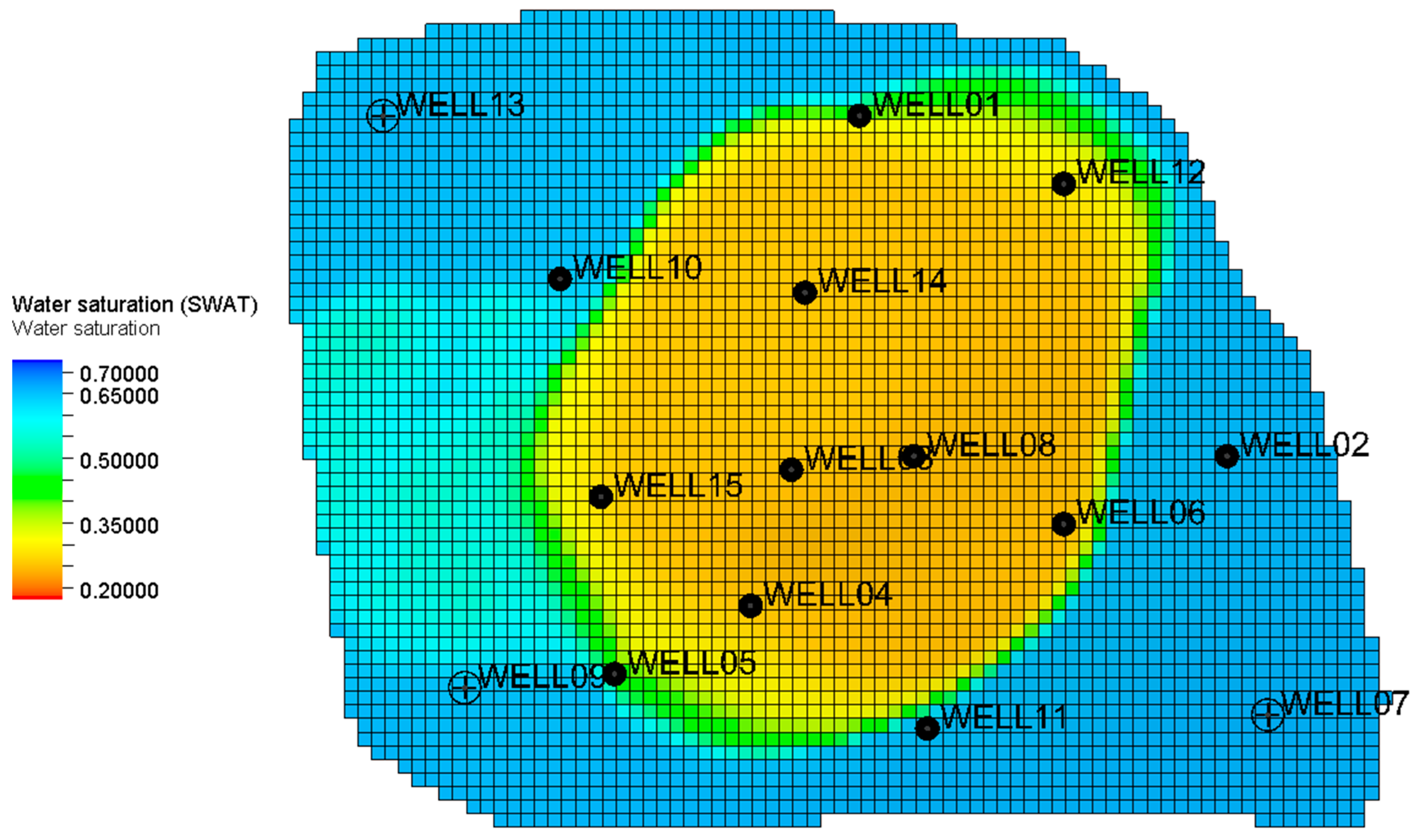
2.2. Reservoir Model Construction

The studied reservoir comprises two distinct productive oil zones that are separated by an impermeable shale layer. Geological investigations have revealed that the reservoir predominantly consists of alternating sandstone and shale sequences. Moreover, the oil zones are partially surrounded by an aquifer. Within this reservoir setting, there are a total of 15 vertical wells, including 12 producers and 3 monitor wells. These wells have been actively producing from both the upper and lower zones since 1997, providing valuable data for reservoir characterization and analysis. The geological model delineates two productive zones separated by an impermeable shale layer, as presented in Figure 1. The formation’s depth ranges from 7500 ft (2286 m) at the center to 8700 ft (2651 m) at the boundary, with an approximate thickness of 1720 ft (524 m). For numerical simulation purposes, the model is discretized into 81 × 60 × 11 grid blocks, with grid dimensions of 200 ft in both the x and y directions. This detailed discretization enables the precise representation and analysis of the fluid flow and reservoir behavior within the geological formation. Core and well log data from 12 production wells were analyzed to populate the reservoir porosity, as shown in Figure 1. The reservoir porosity ranges from 5% (tight rock) to 33% (highly porous medium), with an arithmetic mean of 21%, indicating significant heterogeneity. In this context, a conventional linear correlation between porosity and permeability would not sufficiently characterize the fluid flow in the reservoir. Consequently, more rigorous algorithms are required for an accurate reservoir permeability prediction.

2.3. K-Means Clustering

The K-means clustering algorithm is utilized to extract meaningful clusters from large datasets. This algorithm aims to minimize the objective function of squared distances between clusters [31]. This optimization process enables the algorithm to identify natural groupings or patterns within the data based on the underlying relationships among the variables. By applying the K-means clustering algorithm, it becomes possible to group complex datasets based on underlying relationships among variables within the dataset. This clustering process is particularly valuable in uncovering hidden structures and patterns that may not be immediately apparent through a manual inspection. Clustering analysis often involves using an elbow plot, which aids in determining the optimal number of clusters.

2.4. Hierarchical Clustering

Hierarchical clustering is a data analysis technique that arranges objects into tree-like structures based on their similarities. This method operates using two primary approaches: agglomerative and divisive clustering. In agglomerative clustering, individual data points are initially considered separate clusters and are progressively merged into larger clusters based on their similarities [32]. Conversely, divisive clustering starts with all points in a single cluster and recursively divides them into smaller clusters. The clustering process involves iteratively combining or splitting clusters based on a chosen linkage criterion. Common linkage criteria include single linkage (minimum distance), complete linkage (maximum distance) and average linkage (average distance). These criteria dictate how clusters are merged or split during the hierarchical clustering process. The resulting hierarchical structure is visually represented by a dendrogram, providing valuable insights into the sequence of merging or splitting clusters. However, it is important to note that the computational complexity of hierarchical clustering increases with larger datasets. Additionally, the choice of the linkage method significantly influences the clustering outcome and must be carefully considered. In this study, the “Ward” linkage method was utilized due to its ability to minimize variance within clusters, its sensitivity to different cluster shapes, and its compatibility with the Euclidean distance. This choice of linkage method reflects a strategic decision to optimize the clustering performance and achieve a meaningful cluster formation.

2.5. Supervised Machine Learning Framework in Permeability Determination

After obtaining various clusters using both K-means and hierarchical clustering techniques, a supervised machine learning framework is applied to identify the most suitable machine learning algorithm for each cluster within the dataset. This framework aims to establish relationships between independent variables (including a gamma ray (GR) log, bulk density and porosity) and the dependent variable, which is the logarithm to base 10 of permeability. To evaluate the performance of different machine learning algorithms, a 5-fold cross-validation method is employed. This technique helps prevent overfitting by dividing the dataset into five subsets (folds) and assessing the accuracy of the models on each fold independently. Among the tested machine learning algorithms, those yielding the lowest root mean squared error (RMSE) are selected as the best fit for the dataset.

These algorithms are then utilized to determine correlations and calculate reservoir permeability for all other wells based on the available GR log, bulk density (RHOB) and porosity data. Following the implementation of K-means and hierarchical clustering techniques, the calculated permeability values are upscaled using an arithmetic average technique. Subsequently, these values are incorporated into the structural model using a Gaussian random function simulation, as depicted in Figure 2 and Figure 3. For a more comprehensive understanding of the geological model construction process, detailed discussions were presented by [33,34].

At first glance, both machine learning techniques exhibit a similar permeability range from 25 to 300 mD, corresponding to tight and highly porous rocks, as analyzed in the porosity range. However, permeability propagated by the hierarchical approach clearly delineates three distinct hydraulic flow units in the reservoir: high-permeability regions in dark red, medium-permeability zones in yellow–green and low-permeability areas in blue. The permeability distribution obtained through the K-means technique appears sparse and non-uniform compared to the more coherent and consistent permeability pattern produced by the hierarchical clustering method. By comparing RMSE values and incorporating hydraulic flow unit classification, reservoir characterization using the hierarchical clustering method demonstrates substantial advantages over other methods such as linear porosity–permeability correlations and K-means in capturing reservoir heterogeneity. This highlights the hierarchical method’s ability to provide a more accurate and detailed understanding of reservoir properties; hence, further analyses will be based on permeability predictions generated by a hierarchical method.

In addition to permeability calculations, the reservoir fluid model and rock physics saturation model have been constructed using available PVT data and relative permeability curves from one well within the area. These models contribute to a more comprehensive understanding of the fluid behavior and reservoir properties. To further refine the reservoir model, historical production and pressure data have been carefully analyzed. These data sets were utilized to develop an objective function for conducting a sensitivity analysis and optimization-based history matching. The resulting matched model is instrumental in forecasting optimization, allowing for the evaluation of different development scenarios and strategies to maximize the reservoir performance and recovery. Figure 4 illustrates a schematic representation of the workflow, beginning with data cleaning and progressing until the data are prepared for optimization.

2.6. Proxy Development and Optimization

Achieving a successful history match model is crucial as it forms the foundation for a reliable forecasting tool within an optimization workflow. The process of field optimization begins by implementing the optimal field development strategy derived from the history match model. To expedite forecasting and reduce the computational time, a proxy model is constructed to approximate the behavior of the detailed geological model. This proxy model captures the relationship between the control variables and the cumulative oil production through a mathematical expression.

The advantage of using a proxy model is evident in its ability to significantly reduce the computational burden associated with running numerous forecasting scenarios. Instead of spending hours on hundreds of simulations to identify optimal control variables for maximum oil production, the proxy model streamlines this process.

Furthermore, the proxy model can be subjected to various solvers to determine the most effective optimization algorithm. This flexibility allows for the iterative refinement of the optimization strategy, ensuring robust and efficient decision making in field development. Figure 5 provides a visual representation of the optimization framework, outlining the steps involved in leveraging the proxy model for efficient and effective field optimization [29].

The proxy model undergoes training with 80 samples using the Monte Carlo sampling method and is subsequently validated with 20 validation points. For a comprehensive understanding of the process of constructing and validating the proxy model, a detailed methodology is outlined in [35].

Upon successfully establishing the proxy model, the optimization process is further refined using advanced techniques such as artificial ANN, PSO, and GA optimizers. These optimization algorithms are employed to enhance the field’s cumulative oil production. These algorithms were chosen because they work very well and are suited for solving complex non-linear problems that come with having to optimize field production. In [36], the ANN algorithm was used together with the GA and PSO algorithms to maximize the NPV by optimizing well spacing in a tight and fractured reservoir in Saskatchewan, Canada. The results for this study showed that the ANN-based model resulted in a faster exploration of well spacing and fracture designs as compared to a traditional simulation approach, which required longer simulation runtimes. The PSO algorithm was also found to outperform the GA in convergence speed and convergence at a higher objective function value. The next section provides more detail into the operation of the selected field optimization algorithms.

2.7. Artificial Neural Network (ANN) Optimizer

An ANN is a computational model composed of interconnected layers, including input, hidden and output layers, with nodes or neurons that imitate the functioning of the human brain. These neural networks excel at identifying intricate patterns and solving non-linear problems with exceptional accuracy. The development of a robust neural network model relies on generating a substantial dataset comprising known input–output pairs.

The ANN model learns from past patterns by storing information in the connections between neurons, represented as connection weights [37]. These weights signify the strength of signals between interconnected neurons and the weighted inputs are summed to produce an output. The weight vectors control connections between hidden layers and from the hidden layers to the output layers [29].

Activation functions, mathematical functions applied to neurons, determine their activation levels and a separate function calculates the network’s output. The ANN’s ability to tackle diverse non-linear problems hinges on the number of neurons in the hidden layer and the presence of multiple hidden layers [38]. Figure 6 illustrates a three-layer ANN structure comprising input, hidden and output layers. In this study, an ANN optimizer is utilized to maximize the cumulative oil production in the field using a proxy model, capitalizing on the ANN’s capacity to process complex patterns and optimize outcomes efficiently.

2.8. Genetic Algorithm (GA) Optimizer

A GA is a methodology for solving optimization problems inspired by the principles of natural selection, which drive biological evolution. The GA algorithm operates by selecting individuals from a population as parents and then employing these parents to generate offspring for subsequent generations. This iterative process is iterated multiple times to produce a diverse set of individual solutions. To select members from the population, the fitness of each potential solution is evaluated, determining their suitability for reproduction.

Figure 7 provides a visual representation of the GA algorithm’s workflow, illustrating how it progresses through the selection, crossover, mutation and evaluation stages to iteratively refine and improve solutions [39]. This algorithmic approach mimics the evolutionary process observed in nature, allowing for the exploration of a wide range of potential solutions and the identification of optimal outcomes for complex optimization problems.

The GA algorithm is particularly effective in tackling optimization problems characterized by non-continuous, stochastic or highly non-linear objective functions. Given the study’s focus on enhancing cumulative oil production in the field, the GA optimizer is utilized to pursue this goal within a PETREL (https://www.slb.com/products-and-services/delivering-digital-at-scale/software/petrel-subsurface-software/petrel) and MATLAB (https://www.mathworks.com/products/matlab.html) environment.

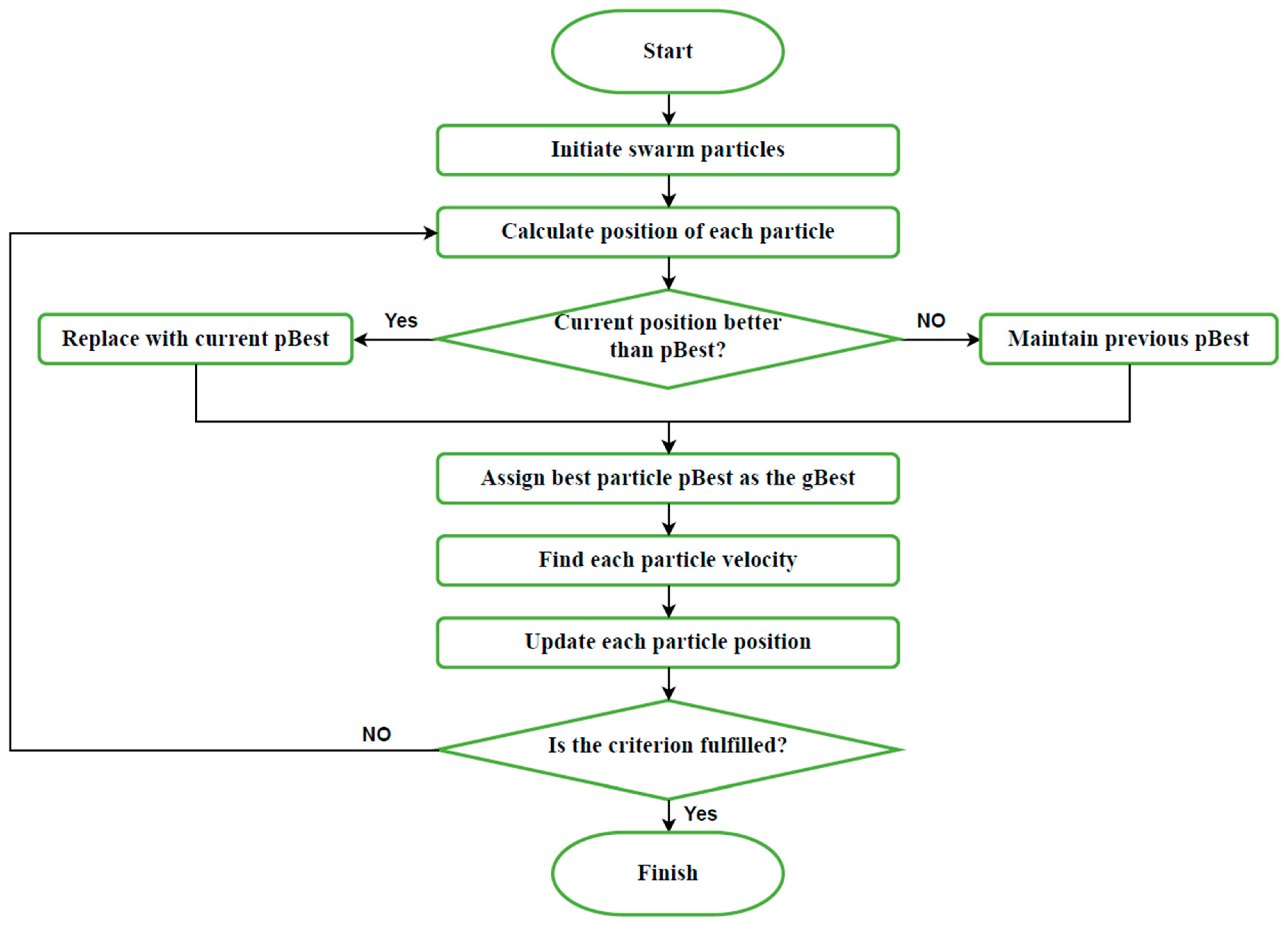
2.9. Particle Swarm Optimization (PSO)

PSO, introduced by [40], operates by repeatedly seeking a solution among potential options guided by a quality-measuring objective function, applicable to numerous optimization tasks. This method is notably cost-effective and offers relatively swift computation times. PSO generates heuristic solutions and employs Swarm Intelligence (SI) principles [41]. The algorithm emulates the collective and decentralized behaviors observed in natural swarms like those of birds and fish. The technique integrates both stochastic and deterministic elements to fine-tune the parameters or candidate solutions, referred to as particles, towards the target objective function [42]. These particles adapt based on personal experience while also considering the movements of their neighbors and the entire group by updating their positions and velocity to reach a global optimum [43].

The process operates by initially updating a particle’s position after assessing the most optimal position it has achieved to date, termed the pBest. Consequently, the position is refined to represent the best outcome since the iteration commenced. Following this, the method evaluates the most advantageous global position or the overall best position within the population, known as the gBest. Subsequently, the velocity is recalculated utilizing both the pBest and gBest values. The particle’s position is then adjusted according to the newly updated velocity. This cycle repeats until a specified termination criterion is met [44]. Figure 8 illustrates the workflow of the PSO algorithm.

Table 2. Comparative analysis of the various optimization algorithms.

	ANN	GA	PSO
Basic Principle	Mimic neural working of the human brain	Based on the principle of natural selection	Collective behavior observed in natural swarms
Mechanism	Composed of interconnected neuron groups, with each connection transmitting signals among themselves	Selects parents from a population to generate offspring for the subsequent generation	An iterative optimization technique that refines solutions based on quality metrics
Strengths	– Can model complex non-linear relationships – Capable of parallel processing – Robust in fault tolerance	– Can find multiple optimal solutions, suitable for multi-objective optimization – Parallel working makes it easily adaptable or modifiable – Robust, easy-to-find global optima without trapping	– Robust and fault tolerant – Adaptable and efficient for dynamic scenarios – Implementation is simple
Weaknesses	– Black-Box nature – Computationally intensive – Requires large datasets compared with other optimizers	– Difficult to configure optimization parameters – Not best suited for solving simple analytical problems – Results highly dependent on how optimization parameters are set	– Sensitive to optimization parameters – Difficult to set optimization parameters – Can struggle to converge on optimal solution

shows a comparison of the field optimization algorithms.

3. Results

The reservoir permeability, determined through the hierarchical clustering technique, serves as the foundation for a case study focusing on optimizing cumulative oil production in both reservoir regions. This case study integrates a machine learning workflow to enhance production outcomes. The ANN optimizer was found to provide the best results for the field cumulative oil production. Before delving into history matching, a sensitivity analysis is conducted to assess the impact of selected input variables on the simulation results. This analysis generates a tornado chart, providing insights into each variable’s contribution to cumulative oil production [45]. Control variables identified for the sensitivity analysis include permeability heterogeneity in different directions, the reservoir pore volume (PV), water–oil contacts in the upper and lower reservoirs, and various aquifer properties such as the initial pressure, depth, permeability, porosity, and external radius.

Figure 9 displays the results of the sensitivity analysis in a tornado plot, offering a visual representation of how changes in each control variable influence oil production. This analysis aids in understanding the key factors driving production variability and guides decision making in optimizing the reservoir performance.

Based on the insights gained from the sensitivity analysis, it is evident that the aquifer properties and PV exert the most significant influence on the simulation model’s outcomes. History matching, an optimization task, aims to minimize the disparity between the simulation results (such as oil and water production) and the actual field data.

Table 3. The most sensitive field variables with relatively higher uncertainties for the history matching process.

		Range of Variation
Variables	Base Values	Minimum	Maximum
PV	1	0.1	1.2
Aquifer pressure (APRESS), psi	3600	3200	4000
Aquifer thickness (ATHICK), ft	12	8	20
Aquifer permeability (APERM), mD	20	10	30
Permeability multiplier in I-direction (PERMI)	1	0.5	2
Permeability multiplier in J-direction (PERMJ)	1	0.5	2
Water–oil contact of upper reservoir (WOC1), ft	−8420	−8430	−8390
Water–oil contact of lower reservoir (WOC2), ft	−8385	−8420	−8380

lists the uncertain parameters identified through the sensitivity analysis, which are crucial for optimization-based history matching. This table includes the ranges representing the maximum and minimum values for each parameter, providing a comprehensive overview of the optimization process. By addressing these uncertain parameters within their specified ranges, the history matching process aims to align simulated results closely with observed field data.

During the optimization-based history matching procedure, the evolution strategy optimizer systematically adjusts individual parameters to minimize the discrepancy between the simulated and observed production data. This iterative process aims to identify the optimal combination of parameters listed in Table 1, which results in the least error when compared to the observed data. The model undergoes 500 iterations to converge towards the best solution by minimizing the objective function. Once the model is calibrated to closely match observed production data with minimal error, adjustments are made to geological properties to enhance the simulation model’s accuracy for future field development processes. Figure 10 and Figure 11 depict the optimal solutions achieved through the history matching process for the oil and water production rate of the twelve production wells and the cumulative production of the entire field. The daily rate and cumulative field production profiles for oil and gas production are indicated with the same color. The distinction in these two profiles can be seen in the shape of the curves. The curves for cumulative production for oil and water can be seen to start from the origin and show a steady increase in production. However, the production rate profiles for oil and water can be seen to vary as the production time increases. Regarding field cumulative production, the calibrated model shows a less than 1% deviation from the historical production data. These figures showcase excellent outcomes after implementing the hierarchical clustering technique. As a result, this permeability estimation was selected for utilization in subsequent field optimization processes. The field permeability calculated after implementing the hierarchical clustering technique proves to be more accurate and reliable in capturing the true reservoir behavior and dynamics, ultimately contributing to an enhanced reservoir performance and productivity.

Table 4. The most sensitive uncertainties for the history matching process for field permeability calculated after hierarchical clustering method.

		Range of Variation
Variables	Matched Values	Minimum	Maximum
PV	0.74	0.1	1.2
Aquifer pressure (APRESS), psi	3200	3200	4000
Aquifer thickness (ATHICK), ft	11.6	8	20
Aquifer permeability (APERM), mD	24.1	10	30
Permeability multiplier in I-direction (PERMI)	0.5	0.5	2
Permeability multiplier in J-direction (PERMJ)	1.9	0.5	2
Water–oil contact of upper reservoir (WOC1), ft	−8430	−8430	−8390
Water–oil contact of lower reservoir (WOC2), ft	−8386	−8420	−8380

shows the final values implemented after history matching for the hierarchical clustering method to calculate the field permeability. These values are automatically applied to the matched model for subsequent field development processes.

4. Discussion

4.1. Optimization Forecasting

To optimize the cumulative oil production in the studied field, comprehensive case studies were executed to assess various field development scenarios, utilizing water flooding as a secondary recovery technique. By utilizing the history match model, we projected the cumulative oil production for the next 15 years based on the outlined development scenarios.

Scenario 1: the initial case involved implementing a standard depletion strategy where all producers continue production at a specified bottom hole pressure, maintaining the existing well types without alteration.

Scenario 2, Water Flooding #1 (WF1): This field development strategy entails the conversion of three pressure observation wells (wells 07, 09 and 13) into injectors positioned along the reservoir boundary’s edge with the highest water saturation. For a visual representation, please refer to Figure 12, which illustrates the water saturation at the conclusion of primary recovery and the precise locations of the three converted pressure observation wells.

Scenario 3, Water Flooding #2 (WF2): This case, similar to Case 2, employs a secondary recovery strategy using water flooding; however, in this scenario, producers are transformed into injection wells. Specifically, three of the highest water-producing wells are converted into water injection wells while maintaining the status for other producers and monitoring wells. Figure 13 illustrates the water saturation distribution in the upper reservoir and the precise locations of the three converted wells (wells 02, 04 and 05). It is worth noting that wells 02 and 05 are situated at the water–oil interface’s edge, while well 04 operates at the water–oil interface in the lower reservoir. This contextual information forms the basis for converting these wells into water injection wells.

Scenario 4, Water Flooding #3 (WF3): This scenario represents a fusion of the previously outlined water flooding plans, where both three observation wells and three of the highest water-producing wells are converted into water injection wells. The specific locations of the injection wells (02, 04, 05, 07, 09 and 13) in this combined scenario are depicted in Figure 14.

To determine the most suitable scenario for field development and optimization, we forecast the cumulative production for the next 15 years using normal depletion, WF1, WF2 and WF3, as illustrated in Figure 15. Normal depletion is ranked the least favorable due to its lower cumulative oil recovery compared to the water flooding plans. This reinforces the preference for a secondary recovery approach in the studied field. While WF1, which involves converting the three highest water-producing wells into injectors, shows the highest field production in the initial 13 years, WF3 demonstrates significantly better results after 15 years of production. Hence, WF3 emerges as the optimal field development plan for long-term production sustainability. The decline in production in the WF1 development strategy could be attributed to early water breakthroughs at the producer wells or even an uneven pressure distribution causing the pressure to decline quickly within the reservoir. In contrast, the additional wells in the WF3 strategy may well have resulted in a more balanced pressure distribution throughout the reservoir to help slow down the breakthrough time at the producer wells leading to additional oil recovery as compared to the WF1 and WF2 strategies.

Table 5. Production comparison of four development plans.

Field Development Strategy	15-Year Production (MMSTB)
Normal depletion plan	19.3
WF1	28.2
WF2	28.8
WF3	29.5

provides a summary of cumulative oil production after 15 years for all four field development scenarios considered.

In typical practice, a water flooding plan is implemented to preserve the pore pressure and maintain the bottom hole pressure above the bubble point pressure. In cases of injection water breakthrough, production wells with the highest water cut are typically shut down. Consequently, five critical constraints were taken into account for forecasting purposes: the production bottom hole pressure, injection bottom hole pressure, voidage replacement, production rate, and water cut. Initially, a sensitivity analysis was conducted on these field operating constraints to assess their impact on the forecasted outcomes. The minimum, maximum, and base values of the sensitive parameters were derived from historical reservoir pressure data, field development insights gathered from a literature review, and a focus on the factors considered to have the greatest impact on oil recovery. These ranges were also set to ensure that reservoir operations remained under the fracture pressure to avoid unintentional breakdown. The global sensitivity analysis was performed, running all factors simultaneously over 100 iterations to determine which parameters had the most significant influence on oil recovery outcomes.

Figure 16 presents the tornado chart derived from the sensitivity analysis results. It is evident from the chart that production bottomhole pressure emerges as the most sensitive control variable in the water flooding process. This tornado chart is particularly important since it provides important insights into the key drivers of the field production. This information is important in helping determine the level of importance to assign to a given parameter when fine-tuning the model for subsequent field optimization processes. Additional time and research would need to go into defining the minimum and maximum values for the optimization phase since it is a parameter that has a very high influence on the developed model.

The forthcoming optimization process is poised to determine the optimal bottomhole pressure that maximizes oil production. This optimization is particularly crucial, especially in unconventional reservoirs, where an excessively low bottom hole pressure can elevate the effective stress and diminish the formation’s effective permeability, consequently reducing the oil recovery potential.

4.2. Field Production Optimization

The WF3 strategy was identified as the optimal development approach, leading to the highest cumulative oil recovery among the considered scenarios. This strategy was then employed for further analysis in optimizing field production. Figure 17 displays the validation cross-plot for the proxy model constructed for WF3. The proxy model was constructed to evaluate the effect of varying the field operating constraints on maximizing the cumulative oil recovery which, in this case, is the objective function. The proxy model was trained with 80 samples using the Monte Carlo sampling method and was then subsequently validated with 20 validation points. The 80-to-20 sample ratio for the training and test data split provides a good balance between the training and the model validation data. When building any model, it is important that enough training samples are provided to make sure that an accurate and representative model is developed. Referring to Figure 17, the training points are indicated by the red cross marks, while the validation points are indicated by the green dots. The plot shows a very good correlation between the training and the validation points, where both these points can be seen very close to the 45-degree line, indicating a high level of accuracy and consistency when deciding to make predictions to determine outcomes with this model.

Utilizing a machine learning proxy makes it convenient to vary these operating constraints, saving on computational time. In this plot, the oil cumulative predictions generated by the proxy model are compared against the results obtained from the full geological model. The validation points depicted in Figure 17 exhibit a notable agreement with the training points, indicating the reliability and accuracy of the proxy model in predicting oil cumulative production for the selected water flooding strategy. This validation process is crucial in ensuring the robustness of the modeling approach and instilling confidence in the forecasted production outcomes.

At the conclusion of the 15-year forecasting period,

Table 6. Operating constraints and field cumulative oil production.

Field Operating Constraints	WF3 Base Case	ANN Optimizer Using Petrel	PSO Optimization Using MATLAB	GA Optimizer Using Petrel	GA Optimization Using MATLAB
Injection BHP, psi	4000	4415	4492	4205	4347
Production BHP, psi	1500	1000	1024	1175	1024
Group production rate control, bbl/d	11000	10000	10133	17789	11824
Voidage	1	1	0.98	0.96	0.98
Water cut	0.9	0.85	0.85	0.77	0.91
Field cumulative oil production (MMstb)	29.5	61.9	59.9	48.9	59.1

provides insights into the operating constraints and the cumulative oil production achieved in the field when employing various optimization techniques such as ANN, PSO, and GA. The ANN optimization conducted in Petrel demonstrates the most substantial enhancement in cumulative oil production compared to the WF3 base case. This signifies the efficacy of ANN in fine-tuning operational parameters for maximizing oil recovery. The ANN algorithm proves why it is highly regarded in solving production optimization problems. The algorithm’s ability to identify nonlinear relationships and fine-tune variables affecting the field operating parameters and the cumulative oil recovery allows it to yield the highest cumulative recovery compared to the other optimization approaches. Following closely, the PSO optimization conducted using MATLAB yields the second-highest cumulative production improvement among the optimization methods considered. All these algorithms prove to perform better than traditional methods and offer significantly higher oil recoveries compared to the base case.

5. Conclusions

This research provides a comprehensive machine learning workflow facilitating reservoir characterization, primary production history matching, field development, and optimizing oil recovery. Two distinct clustering methods were investigated, showing more accurate results in computing reservoir permeability in complex and highly heterogeneous sand-shale sequences compared with linear regression. Among them, the hierarchical method introduced a better prediction of formation property distribution and has been used to improve history matching and optimize oil production.

The use of machine learning-assisted history matching and sensitivity analysis facilitated an understanding of the most sensitive parameters that impact history matching outcomes. This study then assessed various strategies for field development to boost cumulative oil production. The conversion of the field pressure monitoring wells and the three highest water-producing wells resulted in the highest cumulative oil recovery by successfully reducing water production and maintaining the average reservoir pressure prior to optimization. The field production was improved further by leveraging the GA, ANN, and PSO optimizers across different software platforms, with the ANN algorithm outperforming other methods, resulting in higher cumulative oil recovery over a 15-year forecast.

This research provides a comprehensive and complete workflow for utilizing machine learning techniques across all stages, from reservoir characterization and building 3D models to history matching production data, and using machine learning to optimize the operating conditions for maximizing oil recovery. Future studies can build on the findings of this research to propose more field development plans and apply additional machine learning methods beyond GA, PSO, and ANN to achieve higher oil recovery. Based on the foundations of the proposed machine learning-assisted workflow, one can quickly apply it to field development and optimize oil recovery in their formations of interest.

References

1. US Energy Information Administration—EIA, 2023—Independent Statistics and Analysis. Available online: https://www.eia.gov/pressroom/releases/press542.php (accessed on 4 August 2024).
2. Kenzhebek, Y.; Imankulov, T.; Akhmed-Zaki, D.; Daribayev, B. Implementation of regression algorithms for oil recovery prediction. East.-Eur. J. Enterp. Technol. 2022, 2, 69–75. [Google Scholar] [CrossRef]
3. Parhi, B.; Patwardhan, S. Predicting critical parameters of a declining oil well—A data driven approach. ECS Trans. 2022, 107, 10701–10720. [Google Scholar] [CrossRef]
4. Ozigis, M.; Kaduk, J.; Jarvis, C. Mapping terrestrial oil spill impact using machine learning random forest and landsat 8 oli imagery: A case site within the niger delta region of nigeria. Environ. Sci. Pollut. Res. 2018, 26, 3621–3635. [Google Scholar] [CrossRef]
5. Huang, S.; Tian, L.; Zhang, J.; Chai, X.; Wang, H.; Zhang, H. Support vector regression based on the particle swarm optimization algorithm for tight oil recovery prediction. ACS Omega 2021, 6, 32142–32150. [Google Scholar] [CrossRef]
6. Gharbi, R.B.; Elsharkawy, A.M. Neural-network model for estimating the PVT properties of Middle East crude oils. In Situ 1996, 20, 367–394. [Google Scholar]
7. Tariq, Z.; Elkatatny, S.; Mahmoud, M.; Ali, A.Z.; Abdulraheem, A. A new technique to develop rock strength correlation using artificial intelligence tools. In Proceedings of the SPE Reservoir Characterisation and Simulation Conference and Exhibition, Abu Dhabi, United Arab Emirates, 8–10 May 2017; p. SPE-186062-MS. [Google Scholar]
8. Saikia, P.; Baruah, R.D.; Singh, S.K.; Chaudhuri, P.K. Artificial Neural Networks in the domain of reservoir characterization: A review from shallow to deep models. Comput. Geosci. 2020, 135, 104357. [Google Scholar] [CrossRef]
9. Buist, C.; Bedle, H.; Rine, M.; Pigott, J. Enhancing Paleoreef reservoir characterization through machine learning and multi-attribute seismic analysis: Silurian reef examples from the Michigan Basin. Geosciences 2021, 11, 142. [Google Scholar] [CrossRef]
10. Ali, M.; Zhu, P.; Jiang, R.; Huolin, M.; Ehsan, M.; Hussain, W.; Zhang, H.; Ashraf, U.; Ullaah, J. Reservoir characterization through comprehensive modeling of elastic logs prediction in heterogeneous rocks using unsupervised clustering and class-based ensemble machine learning. Appl. Soft Comput. 2023, 148, 110843. [Google Scholar] [CrossRef]
11. Chaki, S.; Routray, A.; Mohanty, W.K. Well-log and seismic data integration for reservoir characterization: A signal processing and machine-learning perspective. IEEE Signal Process. Mag. 2018, 35, 72–81. [Google Scholar] [CrossRef]
12. Hussein, M.; Stewart, R.R.; Sacrey, D.; Wu, J.; Athale, R. Unsupervised machine learning using 3D seismic data applied to reservoir evaluation and rock type identification. Interpretation 2021, 9, T549–T568. [Google Scholar] [CrossRef]
13. Wrona, T.; Pan, I.; Gawthorpe, R.L.; Fossen, H. Seismic facies analysis using machine learning. Geophysics 2018, 83, O83–O95. [Google Scholar] [CrossRef]
14. Huang, L.; Gao, K.; Li, D.; Zheng, Y.; Cladouhos, T. Delineating Faults beneath Basalt at the Soda Lake Geothermal Field. In Proceedings of the 48th Workshop on Geothermal Reservoir Engineering, Stanford, CA, USA, 6–8 February 2023; pp. 6–8. [Google Scholar]
15. Amosu, A.; Sun, Y. Identification of thermally mature total organic carbon-rich layers in shale formations using an effective machine-learning approach. Interpretation 2021, 9, T735–T745. [Google Scholar] [CrossRef]
16. Mishra, A.; Sharma, A.; Patidar, A.K. Evaluation and development of a predictive model for geophysical well log data analysis and reservoir characterization: Machine learning applications to lithology prediction. Nat. Resour. Res. 2022, 31, 3195–3222. [Google Scholar] [CrossRef]
17. Soomro, A.A.; Mokhtar, A.A.; Kurnia, J.C.; Lashari, N.; Lu, H.; Sambo, C. Integrity assessment of corroded oil and gas pipelines using machine learning: A systematic review. Eng. Fail. Anal. 2022, 131, 105810. [Google Scholar] [CrossRef]
18. Liu, Y.; Bao, Y. Review on automated condition assessment of pipelines with machine learning. Adv. Eng. Inform. 2022, 53, 101687. [Google Scholar] [CrossRef]
19. Sun, Q.; Ampomah, W.; You, J.; Cather, M.; Balch, R. Practical CO2—Wag field operational designs using hybrid numerical-machine-learning approaches. Energies 2021, 14, 1055. [Google Scholar] [CrossRef]
20. Makhotin, I.; Orlov, D.; Koroteev, D.; Burnaev, E.; Antonenko, D. Machine learning for recovery factor estimation of an oil reservoir: A tool for de-risking at a hydrocarbon asset evaluation. arXiv 2020. [Google Scholar] [CrossRef]
21. Shirazy, A.; Hezarkhani, A.; Timkin, T.; Shirazi, A. Investigation of Magneto-/Radio-Metric Behavior in Order to Identify an Estimator Model Using K-Means Clustering and Artificial Neural Network (ANN) (Iron Ore Deposit, Yazd, IRAN). Minerals 2021, 11, 1304. [Google Scholar] [CrossRef]
22. Shabani, A.; Ziaii, M.; Monfared, M.S.; Shirazy, A.; Shirazi, A. Multi-Dimensional Data Fusion for Mineral Prospectivity Mapping (MPM) Using Fuzzy-AHP Decision-Making Method, Kodegan-Basiran Region, East Iran. Minerals 2022, 12, 1629. [Google Scholar] [CrossRef]
23. Teixeira, A.F.; Argimiro, R.S. Machine Learning Models to Support Reservoir Production Optimization. IFAC-PapersOnLine 2019, 52, 498–501. [Google Scholar] [CrossRef]
24. Shirangi, M.G. Applying machine learning algorithms to oil reservoir production optimization. In Technical Report. Machine Learning Course Project Report; Stanford University: Stanford, CA, USA, 2012. [Google Scholar]
25. Almasov, A.; Onur, M.; Reynolds, A.C. Production optimization of the CO2 huff-n-puff process in an unconventional reservoir using a machine learning based proxy. In Proceedings of the SPE Improved Oil Recovery Conference, Tulsa, OK, USA, 31 August–4 September 2020; p. SPE-200360-MS. [Google Scholar]
26. Schuetter, J.; Mishra, S.; Zhong, M.; LaFollette, R. Data analytics for production optimization in unconventional reservoirs. In Proceedings of the SPE/AAPG/SEG Unconventional Resources Technology Conference, URTeC, San Antonio, TX, USA, 20–22 June 2015; p. URTEC-2167005. [Google Scholar]
27. Wang, S.; Chen, S. Evaluation and Prediction of Hydraulic Fractured Well Performance in Montney Formations Using a Data-Driven Approach. In Proceedings of the SPE Western Regional Meeting, Anchorage, AL, USA, 23–26 May 2016. [Google Scholar] [CrossRef]
28. Koray, A.; Bui, D.; Ampomah, W.; Appiah Kubi, E.; Klumpenhower, J. Improving Subsurface Characterization Utilizing Machine Learning Techniques. In Proceedings of the SPE Western Regional Meeting, Anchorage, AL, USA, 21–23 May 2023; p. SPE-212952-MS. [Google Scholar]
29. You, J.; Ampomah, W.; Kutsienyo, E.J.; Sun, Q.; Balch, R.S.; Aggrey, W.N.; Cather, M. Assessment of Enhanced Oil Recovery and CO2 Storage Capacity Using Machine Learning and Optimization Framework. In Proceedings of the SPE Europec Featured at 81st EAGE Conference and Exhibition, London, UK, 3–6 June 2019; p. SPE-195490-MS. [Google Scholar] [CrossRef]
30. Belyadi, H.; Haghighat, A. Machine Learning Guide for Oil and Gas Using Python: A Step-by-Step Breakdown with Data, Algorithms, Codes, and Applications; Gulf Professional Publishing: Houston, TX, USA, 2021; pp. 102–103. [Google Scholar]
31. Melo, A.; Li, Y. Geological Characterization Applying K-Means Clustering to 3D Magnetic, Gravity Gradient, and DC Resistivity Inversions: A Case Study at an Iron Oxide Copper Gold (IOCG) Deposit. In Proceedings of the 2016 SEG International Exposition and Annual Meeting, Dallas, TX, USA, 16–21 October 2016; Volume 35, pp. 2180–2184. [Google Scholar] [CrossRef]
32. Fadokun, D.O.; Oshilike, I.B.; Onyekonwu, M.O. Supervised and Unsupervised Machine Learning Approach in Facies Prediction. In Proceedings of the SPE Nigeria Annual International Conference and Exhibition, Virtual, 11–13 August 2020; p. SPE-203726-MS. [Google Scholar]
33. Ampomah, W.; Balch, R.S.; Ross-Coss, D.; Hutton, A.; Cather, M. An Integrated Approach for Characterizing a Sandstone Reservoir in the Anadarko Basin. In Proceedings of the Offshore Technology Conference, Houston, TX, USA, 2–5 May 2016; p. OTC-26952-MS. [Google Scholar] [CrossRef]
34. Nguyen, S.T.; Nguyen, T.N.; Tran, H.N.; Ngo, A.Q. Integration of 3D Geological Modelling and Fault Seal Analysis for Pore Pressure Characterization of a High Pressure and High Temperature Exploration Well in Nam Con Son Basin, a Case Study Offshore Vietnam. In Proceedings of the International Petroleum Technology Conference, Virtual, 23 March–1 April 2021; p. IPTC-21797-MS. [Google Scholar] [CrossRef]
35. Ampomah, W.; Balch, R.S.; Grigg, R.B.; McPherson, B.; Lee, S.; Will, R.A.; Dai, Z.; Pan, F. Co-optimization of CO2-EOR and storage processes in mature oil reservoirs. Greenh. Gases Sci. Technol. 2016, 7, 128–142. [Google Scholar] [CrossRef]
36. Prosper, A.; Azadbakht, S. Application of ANN-Based Proxy and Metaheuristic Algorithms in Well Spacing Optimization in a Fractured Tight Reservoir. In Proceedings of the SPE Nigeria Annual International Conference and Exhibition, Lagos, Nigeria, 31 July–2 August 2023. [Google Scholar] [CrossRef]
37. Sidarta, D.E.; Tcherniguin, N.; Tan, J.H.; Teng, Y. An ANN-Based Model to Artificially Transform a Floating Vessel into a Wave Monitoring Buoy. In Proceedings of the Offshore Technology Conference Asia, Kuala Lumpur, Malaysia, 2–6 November 2020; p. OTC-30246-MS. [Google Scholar] [CrossRef]
38. Santhirasekaran, L.; Ong, D.; Foo, F.K.; Hasiholan, B. Is Artificial Intelligent the Future for AHM? Decision Making between an Automated Optimisation of ANN Proxy versus Full Numerical Simulation Optimisation Technique. In Proceedings of the Society of Petroleum Engineers—SPE/IATMI Asia Pacific Oil and Gas Conference and Exhibition, Virtual, 12–14 October 2021; p. SPE-205808-MS. [Google Scholar] [CrossRef]
39. Ferreira, W.C.; Hilterman, F.J.; Diogo, L.A.; Santos, H.B.; Schleicher, J.; Novais, A. Global Optimization for AVO Inversion—A Genetic Algorithm Using a Table-Based Ray-Theory Algorithm. In Proceedings of the 78th EAGE Conference and Exhibition 2016: Efficient Use of Technology—Unlocking Potential, Vienna, Austria, 29–30 May 2016; Volume 2, pp. 543–547. [Google Scholar] [CrossRef]
40. Eberhart, R.; Kennedy, J. A new optimizer using particle swarm theory. In Proceedings of the MHS’95, Proceedings of the Sixth International Symposium on Micro Machine and Human Science, Nagoya, Japan, 4–6 October 1995; pp. 39–43.
41. Gad, A.G. Particle swarm optimization algorithm and its applications: A systematic review. Arch. Comput. Methods Eng. 2022, 29, 2531–2561. [Google Scholar] [CrossRef]
42. Yang, X.-S. Particle Swarm Optimization. In Nature-Inspired Optimization Algorithms; Elsevier: Amsterdam, The Netherlands, 2014; pp. 99–110. [Google Scholar] [CrossRef]
43. Rhim, H. How Does Particle Swarm Optimization Work?|Baeldung on Computer Science. Baeldung. 2023. Available online: https://www.baeldung.com/cs/pso (accessed on 12 June 2024).
44. Le, L.M.; Ly, H.B.; Pham, B.T.; Le, V.M.; Pham, T.A.; Nguyen, D.H.; Tran, X.T.; Le, T.T. Hybrid artificial intelligence approaches for predicting buckling damage of steel columns under axial compression. Materials 2019, 12, 1670. [Google Scholar] [CrossRef]
45. Bui, D.; Nguyen, T.; Yoo, H. A Coupled Geomechanics-Reservoir Simulation Workflow to Estimate the Optimal Well-Spacing in the Wolfcamp Formation in Lea County. In Proceedings of the AADE 2023 National Technical Conference & Exhibition, Midland, TX, USA, 4–5 April 2023; p. AADE-23-NTCE-014. [Google Scholar]
Figure 1. Porosity distribution populated by density log.
Geotechnics 04 00055 g001
Figure 2. Permeability distribution implementing the K-means clustering method.
Geotechnics 04 00055 g002
Figure 3. Permeability distribution implementing the hierarchical clustering method.
Geotechnics 04 00055 g003
Figure 4. Workflow from start of data cleaning to beginning of optimization.
Geotechnics 04 00055 g004
Figure 5. Workflow of proxy modeling and optimization (after ref. [29]).
Geotechnics 04 00055 g005
Figure 6. A three-layer ANN structure.
Geotechnics 04 00055 g006
Figure 7. Flowchart of GA algorithm (after ref. [39]).
Geotechnics 04 00055 g007
Figure 8. Particle Swarm Optimization (PSO) Workflow.
Geotechnics 04 00055 g008
Figure 9. Tornado chart for sensitivity analysis of the uncertainties.
Geotechnics 04 00055 g009
Figure 10. History matching of oil and water production rate of individual wells after implementing hierarchical clustering method.
Geotechnics 04 00055 g010
Figure 11. History matching of the cumulative production of the whole field after implementing hierarchical clustering method.
Geotechnics 04 00055 g011
Figure 12. Water saturation map at the end of primary recovery and location of three converted wells in water flooding #1.
Geotechnics 04 00055 g012
Figure 13. Water saturation map at the end of primary recovery and location of three converted wells in water flooding #2.
Geotechnics 04 00055 g013
Figure 14. Water saturation map and location of three converted wells in water flooding #3.
Geotechnics 04 00055 g014
Figure 15. Comparison of cumulative oil production in 15 years of the presented scenarios.
Geotechnics 04 00055 g015
Figure 16. Tornado chart for sensitivity analysis of the water flooding control variables.
Geotechnics 04 00055 g016
Figure 17. Validation plot for the proxy model of WF3.
Geotechnics 04 00055 g017