Evaluating Sand Particle Surface Smoothness Using a New Computer-Based Approach to Improve the Characterization of Macroscale Parameters

Abstract

The analysis of sands, and the foundation systems with which they interact, are largely dependent on macroscale behavioral parameters that represent the aggregated response of several microscale characteristics. This research paper examines the influence of surface texture, or smoothness, on the behavior of sands. The challenge of estimating or measuring smoothness, due to its microscale feature domain, is addressed through an examination of six artificially graded sand specimens. These specimens are evaluated both visually and numerically to characterize their surface smoothness. The first approach described is a simple visual method that uses a smoothness scale consistent with those of roundness and sphericity. This method, which can be performed with a tool as simple as a hand lens, evaluates a group of representative particles collectively. The second approach is also a visual evaluation, but it utilizes images obtained via scanning electronic microscopy, traditional optical microscopy, and newer low-cost digital microscopes that can be rapidly connected to a smartphone or laptop. To validate these visual estimates, a novel third approach is introduced. This approach is a more objective numerical analysis measurement technique that enables rapid and economic quantification of smoothness. This technique may assist both practitioners and academics in their understanding of the macroscale response of coarse-grained soils. In addition to the visual methods, this research also conducted several laboratory index tests to observe the mechanical behavior of the specimens, considering their particle shape and surface smoothness properties. The results indicate that angular sands have greater minimum and maximum void ratios, a larger difference between the minimum and maximum void ratios, greater critical state friction angles, and greater flow rates through an orifice of fixed size. When adjusted for surface smoothness using the proposed approach, the behavior of the sands—particularly the limit void ratio results—appears to be more predictable in some cases. These results provide additional evidence of particle smoothness contributing to the strength behavior of sand, which may be particularly useful in the domains of slope stability, land reclamation, soil–structure interaction, and soil dynamics.

1. Introduction

In addition to roundness, R, and sphericity, S, the surface smoothness of sand particles contributes to particle-to-particle interference during shearing. These particle shape and texture properties, in turn, influence the friction angle, compressibility, and other behaviors of the sand. However, surface smoothness, s, has only received modest attention, and it seems that its characterization has largely been ignored due to challenges in obtaining this parameter. This study considers the same six artificially graded specimens, passing the #30 (0.600 mm) sieve and retained on the #40 (0.425 mm) sieve (P30-R40), as those in the work of Muszynski and Vitton [1]. The considered sands included glass beads, Ottawa sand, Manistee dune sand from Manistee, Michigan, Traverse City sand collected from Traverse City, Michigan, Gay stamp sand from the former Mohawk and Wolverine stamp mill in the village of Gay, Michigan, and a crushed limestone sand specimen. We should note the addition of several new sands in the context of these surface smoothness evaluations beyond what was carried out previously by the authors [2]. The grading of the soils by sieve was performed to limit the number of variables, as there may be an additional relationship between the size of the particle and its smoothness in the overall macroscale response. Future research will focus on expanding the range of particles sizes considered.

Smoothness, s, was estimated for these specimens using two broad approaches: (1) a proposed quantitative and/or qualitative visual classification scale (either for evaluating a number of individual particles, or for rapidly evaluating a small specimen of representative particles collectively), and (2) a newly developed numerical routine, using open-source software, designed to quantify surface texture and intended to be useful in validating/checking the results of the visual evaluation approaches. Note that a simple approach for optical/visual evaluation of s (using a hand lens and/or naked eye) was previously described by the authors [2]. That study involved two of the same specimens (glass beads): one with its “default” smooth surface finish, and the other with its surface etched to create a noticeably rough finish. This current study continues the same theme by evaluating additional sand specimens for the purpose of further considering this approach, and others for evaluating s.

Quantification of overall particle shape (i.e., the features of the particle) is generally limited to evaluating angularity or roundness, R, and sphericity, S, where a number of researchers have provided a description of these shape parameters [3,4,5,6,7,8,9]. R describes how sharp or abrupt the edges of a particle are, while S describes the extent to which the sand particle is spherical as opposed to ellipsoidal or oval-shaped. The nomenclature associated with the R and S values is shown qualitatively, with associated numerical indicator values, in

Table 1. R classification values.

Classification a (with Symbol)	Average R a
Very angular (VA)	0.15
Angular (A)	0.20
Subangular (SA)	0.30
Subrounded (SR)	0.40
Rounded (Rnd)	0.60
Well rounded (WR)	0.85

^a Classification and average R provided based on R intervals [6].

and

Table 2. S classification values.

Classification a (with Symbol)	Average S b
Circular (C)	0.85
Semi-Circular (SC)	0.60
Semi-Elongated (SE)	0.40
Elongated (E)	0.20

^a Nomenclature [15]. ^b Average S based on intervals [9].

, respectively. Visually classifying the parameters R and S is relatively simple and reasonably repeatable [1,3,10,11,12,13], since they represent the larger-scale features of a grain of sand or gravel. Additionally, Altuhafi et al. [14] compiled a database of the mechanical behavior of 25 natural sands, specifically considering the effects of particle shape. While this research noted several correlations between key macroscale parameters, it did not find any clear relationship considering smoothness. This may have been due to the potential relationship between particle size and smoothness. Finally, we note that there are indeed certain measurement techniques available which are more extravagant, and may yield automated results (e.g., [15]). The research presented in this paper finds an initial correlation between smoothness and several parameters, using a variety of visual and computational techniques.

2. Particle Smoothness: Proposed Visual Approach

The determination of particle smoothness, s, involves the observation and evaluation of surface texture on a relatively small scale. Even though s is challenging to quantify, work by several researchers has shown that particle texture does play a role in the behavior of particulate materials. For example, Santamarina and Cascante [16] demonstrated that increasing surface roughness decreased small-strain contact stiffness (between grains) while increasing large-strain interparticle friction. Payan et al. [17] established a relationship between the small-strain shear modulus and particle shape parameters and grain size distributions. Alshibli and Alsaleh [18] showed that, under plane strain conditions, sands with rough surface textures exhibited a larger peak friction angle and dilatancy angle for the specimens considered. Based on a historical background study on soil’s aging effects [19], surface texture appears to be a factor in the amount of improvement of properties gained through aging. For these reasons, the practicing engineer should, at a minimum, be aware of particle texture/smoothness effects on field tests and soil behavior.

The authors [2] previously explored techniques concerning both etched and unetched glass bead specimens. The surface smoothness of these particles was estimated using a method that began with a visual comparison, guided by Figure 1. With the glass beads, distinctions were made based on the general appearance: the unetched beads were characterized by a highly glossy surface, whereas the etched beads presented a frosty appearance. These differences were discernible through a hand lens, or even with the naked eye. Further analysis was conducted on both etched and unetched glass beads by subjecting them to magnified SEM (scanning electron microscope) imaging. This allowed for a more objective evaluation of their surface smoothness. Throughout the investigation, a central question emerged: “how close is close enough?” This question encapsulated the challenge of defining precise criteria for smoothness evaluation and remained a guiding inquiry throughout the study. Here, in this current study, the technique is extended to non-glass-bead specimens. The term smoothness, s, is an attempt to retain consistency with the scales used with R and S. Quantitative and qualitative estimates of s (described using a numerical index scale and description, respectively), along with the associated nomenclature, are proposed; for example, 0.1 represents a very rough or an unsmooth surface texture (low smoothness; LS), and 1.0 represents a very smooth surface texture (high smoothness; HS).

The first method for visual evaluation involves observing the surface texture of particles on SEM images and estimating the smoothness based on those observations. Using an optical microscope (as in the second method described later), s can be categorized by examining the appearance of the particle surfaces with modest magnifications (e.g., 30–50×). Note that if the magnification is too great with either the SEM or the optical microscope method, the surface texture will always appear rough. This seems to remain one of the most important aspects of evaluating s (i.e., “how close is too close?”). Note that with SEM images, very fine details may be observed, if desired (Figure 1).

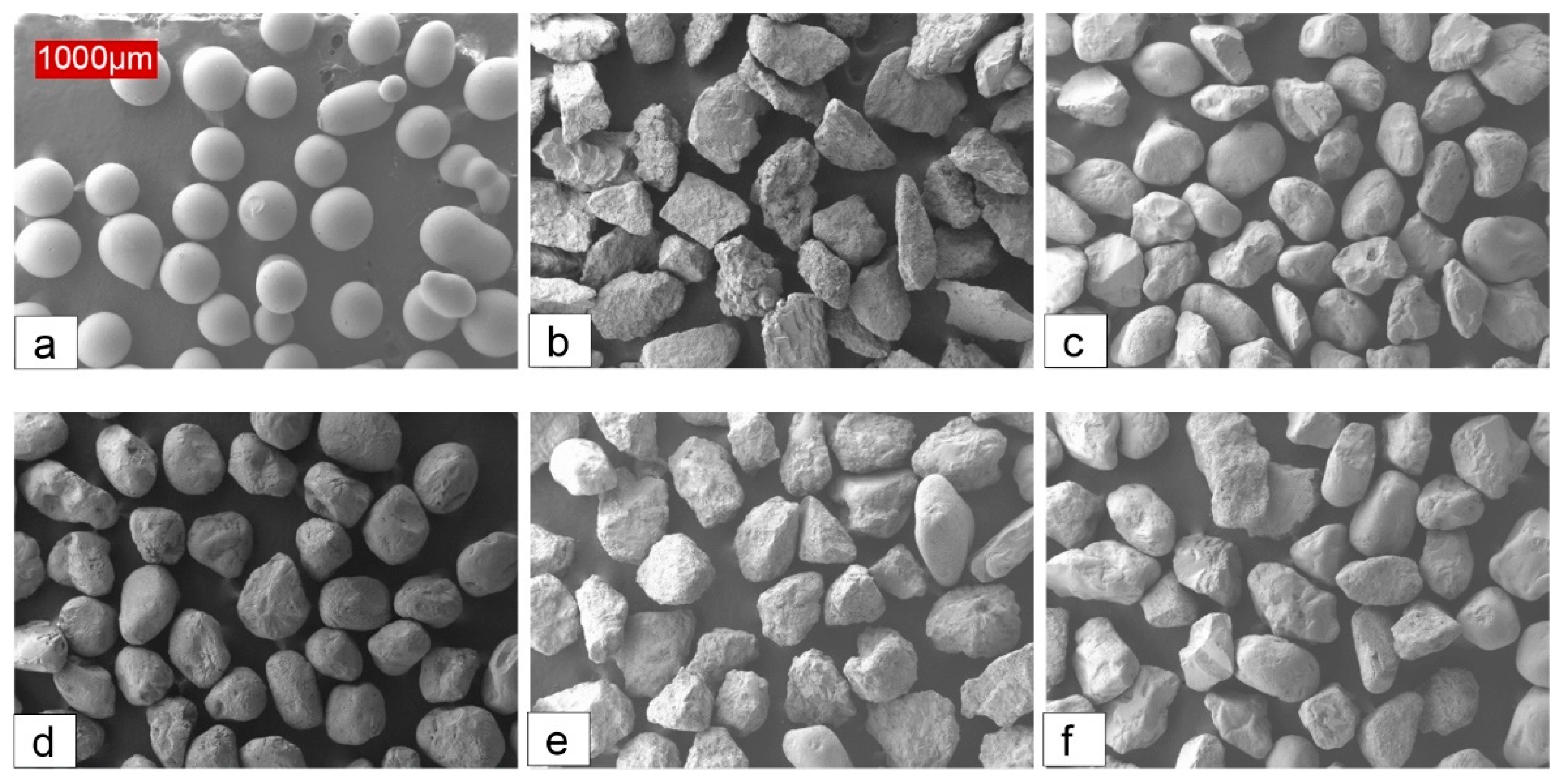
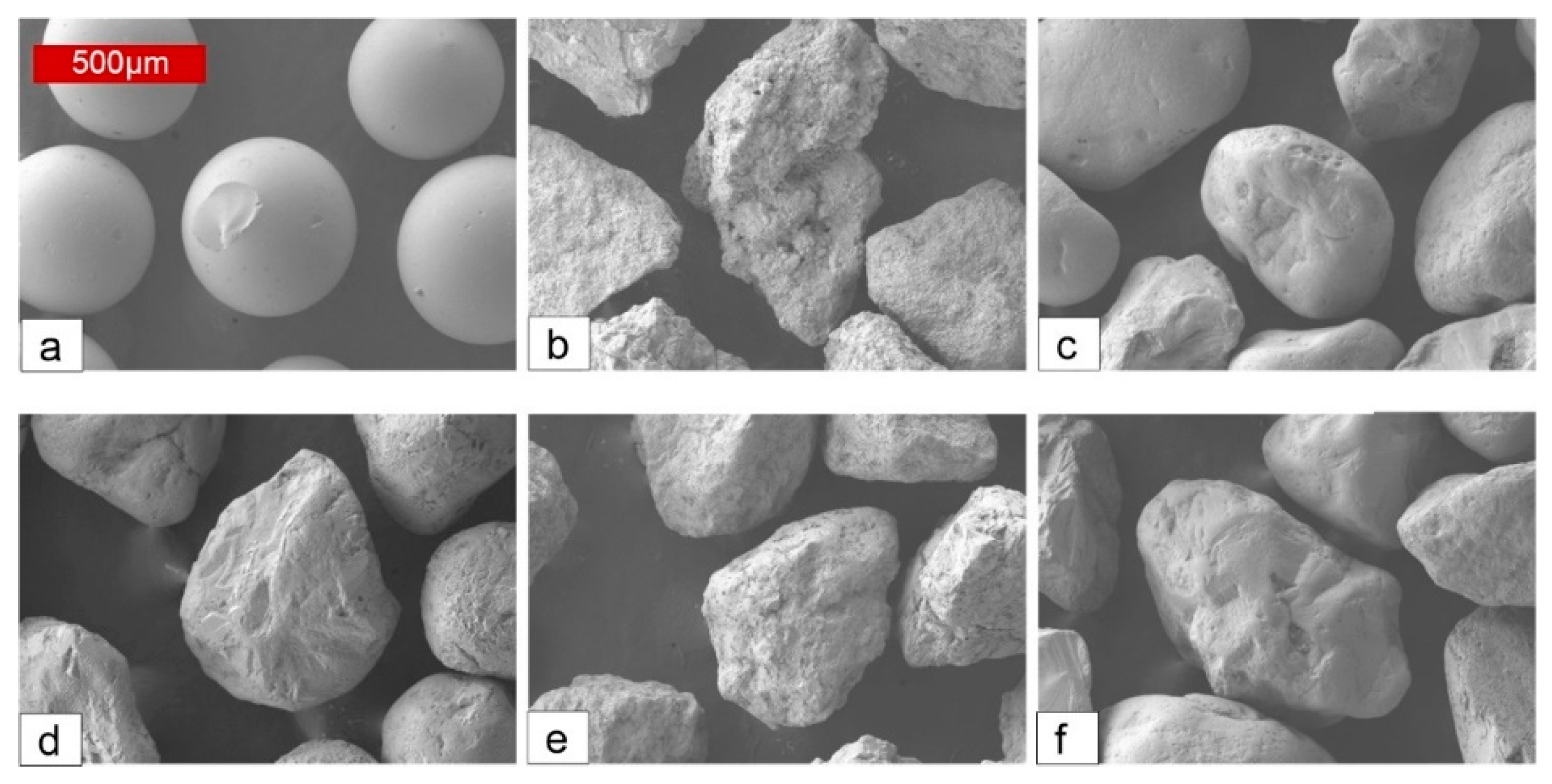
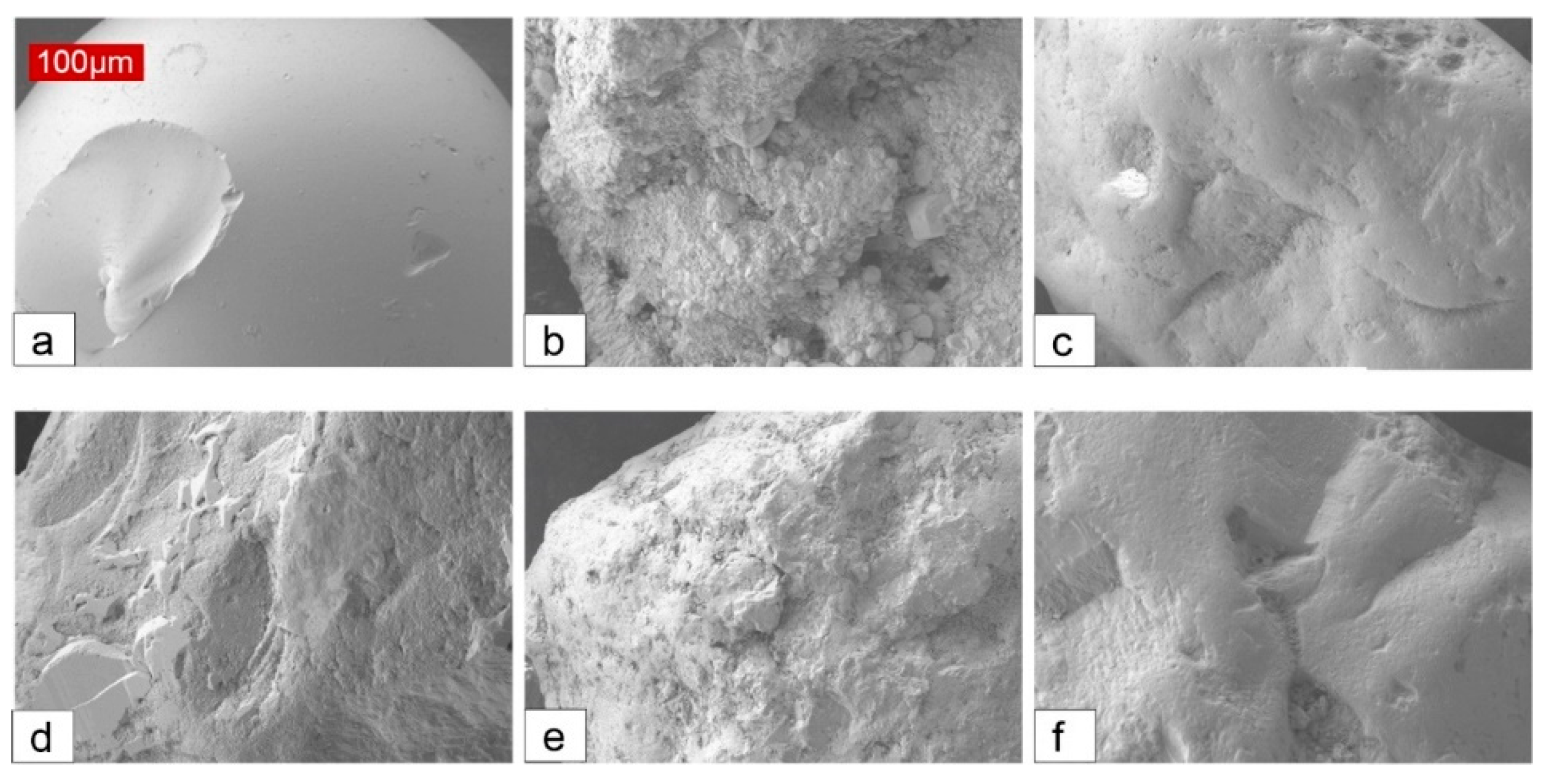
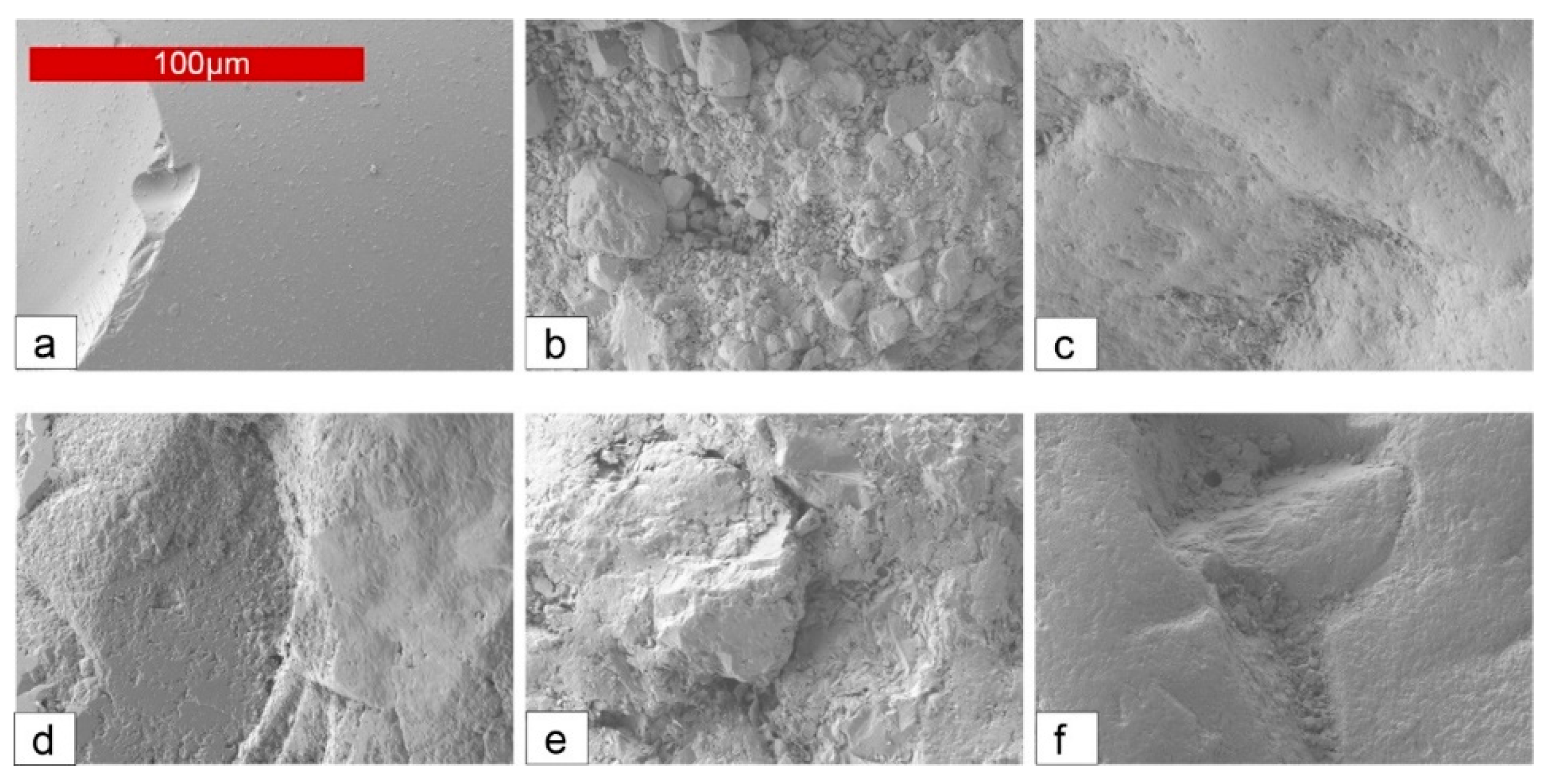
2.1. SEM-Image-Based Visual Approach

The evaluation of particle surface texture through SEM images involves an analysis of small-scale ridges and aberrations present on the surface of the particles. This analysis is informed by the varied levels of shading perceptible within the image. In SEM images, shading or greyscale is the method employed to represent depth, providing a nuanced view of surface irregularities. The proposed scale or guide for qualitatively evaluating these SEM images, as applied to the specific context of this study, is depicted in Figure 1.

Figure 2, Figure 3, Figure 4 and Figure 5 show example SEM images at different magnifications, from 50× to 1500×. The authors judged that the 50× image (Figure 2) likely resulted in the most reasonable visual assessment of s for these particles. At greater magnification, it becomes increasingly challenging to discern the surface texture on the correct scale (as most particles/surfaces begin to appear pitted and/or rough at increasingly high magnifications). Similarly, at low magnification, surface details are no longer visible. What is important, therefore, is not the magnification value itself, but rather the context and, by extension, the number of particles visible in each image. The authors suggest that for a reasonable visual estimate of smoothness, 10 to 30 representative particles should be visible within the frame of an image or observation with magnification of about 50×.

The results of the s estimates by the authors observing 30 individual particles using SEM images are shown in

Table 3. Smoothness estimates by the authors (visual method with SEM images and optical microscope images, numerical analysis, and collective visual assessment).

	Glass Beads				Crushed Limestone				Manistee Dune Sand
	Vis-SEM a	Num b	Vis-opt c	Vis-opt2 d	Vis-SEM	Num	Vis-opt	Vis-opt2	Vis-SEM	Num	Vis-opt	Vis-opt2
Particles observed	30	30	--	30	30	30	--	30	30	30	--	30
Mean	0.95	0.95	0.95	0.93	0.25	0.25	0.20	0.29	0.71	0.71	0.70	0.65
Standard deviation	0.02	0.07	--	0.04	0.09	0.34	--	0.11	0.12	0.18	--	0.13
Coefficient of variation	0.02	0.07	--	0.04	0.36	1.36	--	0.38	0.17	0.25	--	0.20
Minimum	0.90	0.67	--	0.80	0.08	−0.47	--	0.15	0.45	0.21	--	0.45
Maximum	0.98	1.04	--	0.98	0.40	0.81	--	0.60	0.95	0.73	--	0.91
Median	0.95	1.0	--	0.94	0.25	0.29	--	0.28	0.70	0.73	--	0.60
	Ottawa Sand				Gay Stamp Sand				Traverse City Sand
	Vis-SEM	Num	Vis-opt	Vis-opt2	Vis-SEM	Num	Vis-opt	Vis-opt2	Vis-SEM	Num	Vis-opt	Vis-opt2
Particles observed	30	30	--	30	30	30	--	30	30	30	--	30
Mean	0.60	0.58	0.40	0.54	0.33	0.32	0.15	0.29	0.62	0.63	0.50	0.60
Standard deviation	0.10	0.20	--	0.08	0.13	0.26	--	0.18	0.14	0.20	--	0.18
Coefficient of variation	0.16	0.34	--	0.15	0.39	0.81	--	0.62	0.23	0.32	--	0.30
Minimum	0.40	0.14	--	0.38	0.14	−0.21	--	0.12	0.32	0.07	--	0.20
Maximum	0.75	0.91	--	0.55	0.80	0.33	--	0.65	0.93	0.89	--	0.60
Median	0.60	0.59	--	0.55	0.30	0.33	--	0.20	0.67	0.68	--	0.60

^a Visual estimates using SEM images; individual particle evaluation. ^b Measurements using numerical analysis approach (R_tm); individual particle evaluation. ^c Visual estimates using optical microscopy images; specimens evaluated collectively, all with a single observation. ^d Visual estimates using optical microscope images; individual particle evaluation.

noted as “Vis-SEM”.

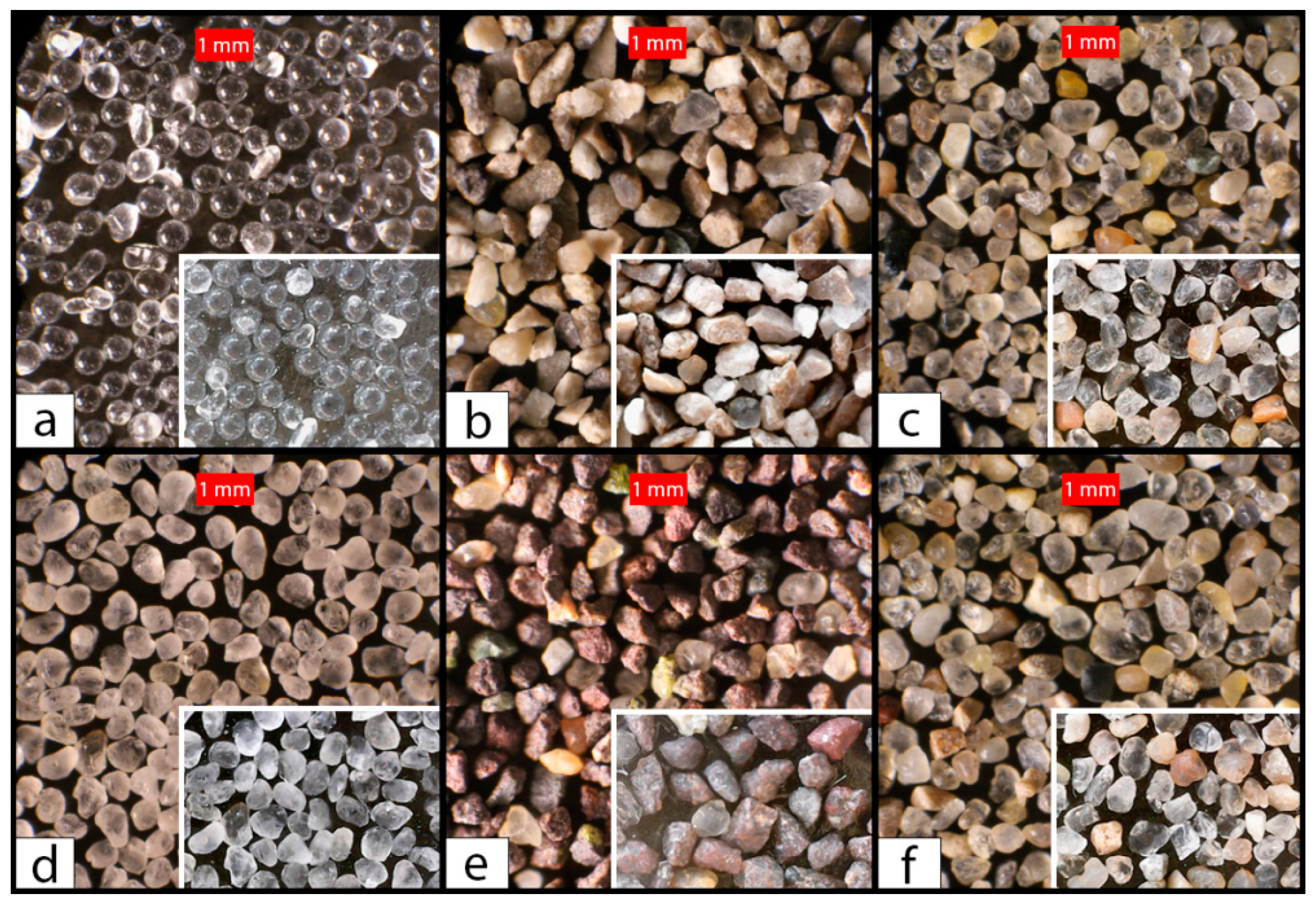
2.2. Optical Microscopy Imagery-Based Visual Approach

The second method for visually evaluating s includes observing particles through an optical microscope at relatively low power and visually evaluating their surface appearance. This approach may be undertaken either by evaluating numerous individual particles (finally arriving at a mean, median, etc., with statistical results, as desired), or by evaluating a small selection of representative particles collectively (i.e., all at once). With the latter approach, a single average—or sometimes an estimated range—of s is assigned by the observer. Furthermore, optical images may be used (obtained by an optical microscope of some type), or a hand lens may be used to view the particles collectively. The use of an optical microscope has recently become a rather interesting proposition. as this option is now further enabled by the recent availability of ultralow-cost digital microscopes, which bypass the need for an expensive traditional optical microscope. Additionally, an increasing percentage of smartphones are capable of macrophotography, which potentially extends the viability of this method to a wider audience. Unlike SEM, which uses a focused beam of electrons to create the image of particles, an optical microscope or camera uses the reflection of light to produce images as observed by the eye. Figure 6 shows traditional optical microscope images of the six 30–40-graded specimens considered in this preliminary study, with images obtained via a low-cost (i.e., approximately 20 USD) USB microscope inlaid for comparison. Figure 7 shows unedited USB microscope images of the crushed limestone and Traverse City samples (b and f, respectively, in Figure 6).

The traditional microscope images were obtained via a manual benchtop microscope using a digital camera lens adapter. Multiple sequential images were recorded, with the focus shifted gradually in each image. The first image in this sequence was obtained with the features of the particles closest to the camera in focus. The focal point was then shifted away from the camera incrementally until the features furthest from the camera were recorded. The series of images were focused and stacked using the automated focus stacking feature in Adobe Photoshop to obtain the final image. This process was labor-intensive and involved a controlled lighting environment, as slight shifts in the ambient light conditions would alter the exposure of the image and prevent stacking. This is in contrast to the low-cost USB microscope images, which were obtained in a matter of seconds under ambient light conditions. While most of the low-cost microscopes contain internal LED lighting, it is too harsh and produces overexposed images. Simple ambient lighting, as shown in Figure 7, captures the surface features of the soil particles at a quality level approximately equivalent to that of the traditional method.

With the differences between SEM and optical microscopy in mind, and with the lower magnification associated with optical microscopy, the proposed classification guide using a microscope of some type, or a hand lens, is as follows: If, through the microscope or hand lens, the particles appear polished and glossy with a high luster, s is likely to be relatively high (high smoothness, HS; s = 0.7 to 1.0). If the particles appear highly frosted, with no visible sheen, the particles likely have a low s level (low smoothness, LS; s = 0.1 to 0.3). If the particles are moderately shiny or appear to have a greasy texture, s is likely to be somewhere between high and low (moderate smoothness, MS, s = 0.4 to 0.6). Note that the technique for visually evaluating surface smoothness varies depending on the mineralogy of the particles. For example, if the particles are predominately those of a translucent mineral (e.g., quartz, topaz, olivine, etc.), the glossy-to-frosted appearance may control the evaluation. If, on the other hand, the particles are of a comparably opaque mineral (e.g., basalt- or limestone-derived), the presence of small-scale ridges or highly visible texture becomes an important clue (more than the level of apparent gloss, etc.).

Table 4. Smoothness (s) classification values.

Texture Classification for Optical Microscope (with Symbol)	Range of s	Average s
Noticeably rough surface/highly frosted, with small ridges and/or very dull appearance (LS)	0.1 to 0.3	0.20
Moderately smooth surface/mildly frosted–greasy appearance (MS)	0.4 to 0.6	0.50
Very smooth surface/polished or highly glossy appearance (G)	0.7 to 1.0	0.85

shows a summary of the proposed s classification system using the microscope and hand lens methods of observation, with descriptions pertaining to both translucent and opaque minerals. We should note that the physical descriptions in Table 4 supplement the visual key shown in Figure 1 for use in the evaluation of SEM images. However, descriptions pertaining to their reflection or scattering of light cannot be extended to SEM evaluations.

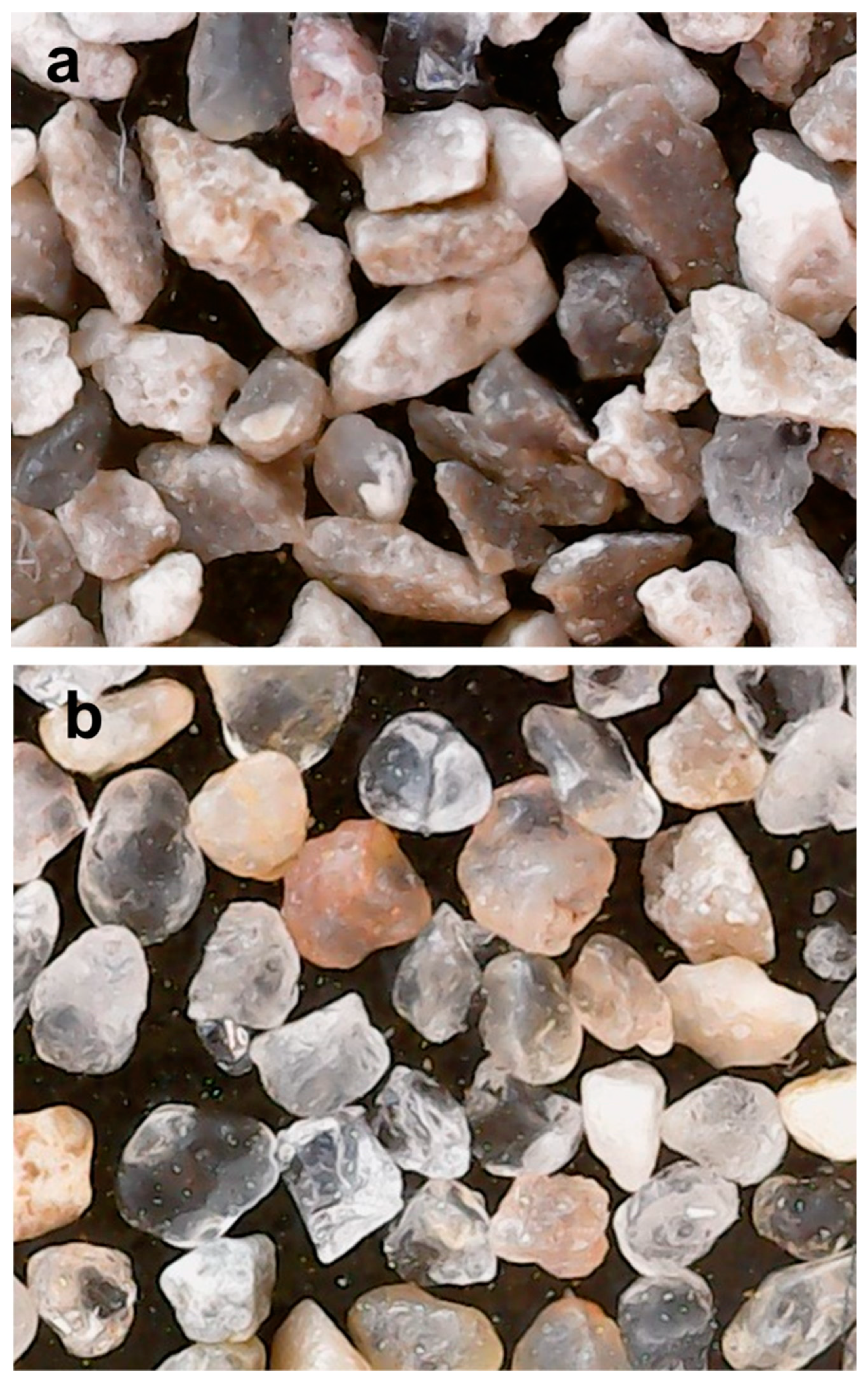
2.2.1. Optical Microscope Imagery or Hand Lens on a Large Number of Particles Collectively

The first approach in this visual method included an evaluation of s values for the optical images by evaluating the overall appearance of the particles (Table 3) contained within the image frame. This approach has an obvious caveat, in that the human eye is likely only able to perceive features down to about 1/10 of a millimeter. And considering a magnification of 10× using a hand lens, it seems reasonable that the human eye may be able to barely discern a feature that is about 10 μ. However, even this level of resolution is likely unable to directly identify most surface features of a particle that could be in the order of 1μ. It is for this reason that the authors propose an indirect approach for observing surface smoothness (i.e., using the appearance of the particles to infer the likely particle surface smoothness).

Table 5. Average smoothness (s) estimates (visual method with optical microscope).

Soil Name	s Estimated Range a	smean a
Glass beads	0.90–1.0	0.95
Ottawa sand	0.30–0.50	0.40
Manistee dune sand	0.60–0.80	0.70
Traverse City sand	0.40–0.60	0.50
Crushed limestone	0.10–0.30	0.20
Gay stamp sand	0.10–0.20	0.15

^a Visual estimate using optical microscopy images on many particles, collectively.

shows the s estimates by the authors using the visual approach for optical microscopy using the collective evaluation approach (where all of the particles are rapidly evaluated rather than individually evaluating each particle). Note that, in Table 5, the collective visual estimate of the specimens resulted in a natural preference for the operator to provide a range of values. We then took the average of that range to arrive at the mean, as noted in Table 5. The mean s results for this first approach are included in Table 3 as “Vis-opt” for comparison with the other techniques.

2.2.2. Optical Microscope Imagery-Based Visual Approach for Numerous Individual Particles

The second approach for the visual evaluation technique included evaluating 30 randomly selected particles, each for its own individual s estimate. The average s results from this individual particle assessment are shown in Table 3, where they are noted as “Vis-opt2”.

The results of the optical microscope imagery-based estimates, as well as those of the evaluation of SEM images are presented in box-and-whisker format in Figure 8. Note that the median value is included (rather than the mean), as would be conventional for most bar-and-whisker plots, along with minimum and maximum values, and finally the 1st and 3rd quartiles.

2.3. Proposed Software-Based Numerical Approach for Numerous Individual Particles

The authors sought a new, simplified method for quantifying particle smoothness using a numerical routine for SEM images. Other researchers have contributed to this work in considerable detail. For example, Alshibli and Alsaleh [18] presented a rather rigorous program involving surface roughness measurements of sand grains using the optical interferometry approach as well as a scanning electron microscope.

In this study, the authors used Gwyddion, which is a free program for scanning probe microscopy (SPM) data’s visualization and analysis. Although the program is specifically designed for the analysis of height fields obtained from SPM data, it can also be used for general greyscale image processing, which is how depth and, therefore, texture are represented in SEM images. Very fine topographic measurements of soil particles were carried out to arrive at representative values describing the surface texture. The images contained within Figure 1 were used to verify/calibrate the approach, wherein the s parameters were obtained for each specimen and the upper and lower bounds were set to smoothness values of 0.9 and 0.1, respectively. The visually obtained estimates and correlated values agreed well for the intermediate points. In order to provide additional data points for the calibration process, the same approach was then used for the SEM images contained in Figure 2 (i.e., 50× magnification as the preferred view for this visual approach), with the upper and lower bounds for smoothness set with the estimated values obtained from the glass beads and crushed limestone, respectively. The average values of 30 representative particles from each specimen for the software approach were compared with the visual SEM estimates. Linear regression was used to link the smoothness estimates and the software roughness parameter (average height of the roughness, R_tm) obtained for the total area of each particle, resulting in a line of best fit with an R² value of 0.998. The individual data points from the numerical analyses were then converted using the linear regression and compared to the corresponding individual visual SEM estimates described in Section 2.1.

The results of the numerical analysis described above are shown in Table 3 (as “Num”), as well as in Figure 8 in box-and-whisker format, along with visual estimates from both the SEM images and traditional optical microscopy images. Note that all three approaches have a relatively consistent median value (Figure 8), along with consistent mean values (see Table 3). However, the upper and lower bounds of the numerical approach exceed the limits of the smoothness scale, going slightly above 1.0 in a few instances and well below 0 in others (Figure 8). This is likely due to the method by which the software analyzes surface smoothness, which calculates the average height of the roughness, R_tm (i.e., the average height of an asperity). In the smooth cases, values of s slightly above 1.0 are likely due to very small changes in the R_tm value, as the obtained linear regression equation is sensitive on the high end. While in theory, R_tm should be 0 for a smoothness of 1.0, as shown in many of the SEM figures (e.g., Figure 4a and Figure 5a), a portion of the laboratory-made glass beads had some surface artifacts. This discrepancy was rather small and only manifested in a handful of instances where the observed beads did not contain significant micro-asperities in the analysis area. On the other hand, the smoothness results on the other end of the scale went well below 0 in several instances. This was again likely due to the method by which smoothness was evaluated, which considered the average height of the roughness, R_tm. Since this is a measure of the relative average height of an asperity, the software is indeed calculating a valid measurement. However, at some point, an increase in the average height of an asperity has no additional effect on the surface roughness. For example, consider the height of the teeth on a saw blade. Increasing the height of the teeth would increase the engagement and function of the saw starting from zero but would eventually reach a point of diminishing returns, analogous to these sand particles under consideration. Thus, the software calculates valid measurements, but they are beyond the point of impact. To better illustrate these results, Figure 8 includes the raw smoothness estimates based on the empirical line of best fit for the software-based data, highlighting the regions above 1.0 and below 0 in a red tint. For practical purposes, data points from these regions would be set to the corresponding upper and lower bounds of the smoothness scale. However, the use of the software-based approach is meant to be an objective verification exercise to support the visual estimate methodology, as it bypasses human biases.

Although this method is simplified and can be used to characterize smoothness, provided that an upper and lower bound can be established from an image set obtained using the same equipment, it is of moderate use to practicing engineers and of limited use to academics, where a more rigorous approach is likely desired. This approach cannot be used for optically obtained images, as the chromatic information contained within photographs would confound the analysis of high and low areas, where a shadow could be used to infer contour. For example, a highly polished piece of granite would contain significant color contrast despite being relatively smooth. In spite of these limitations, the results obtained from these trials were compared with the microscopy data, as described earlier, demonstrating the objective usefulness of said visual methods in the rapid, economical, and meaningful characterization of surface smoothness.

3. Evaluating Overall Particle Shape

Cho et al. [3] used a parameter relating both R and S to one another: regularity (ρ). Regularity is the average of R and S of the particles (Equation (1)). Note that the parameters R and S are defined by [3,6,7,8], among others. The R parameter may be summarized as a measure of particle angularity. Mathematically, R may be determined by taking the ratio of the mean radius of individual inscribed corners/features to the maximum inscribed circle within the particle. Sphericity, S, may be summarized by the ratio of the diameter of the maximum inscribed circle to that of the minimum circumscribed circle.

ρ = (R + S)/2

(1)

Tessari et al. [2] put forth a particle shape parameter including R, S, and s: modified ρ, or ρ_mod. This parameter is the average of R, S, and s, as shown in Equation (2):

ρ_mod = (R + S + s)/3

(2)

Equation (2) indicates that ρ_mod treats R, S, and s as contributing equally to soil behavior in terms of particle shape, and we consider this parameter further in this study. Both ρ and ρ_mod are examined later in the context of the laboratory index testing results for these sands. Also, note that ρ_mod was evaluated using the smoothness obtained from two sources—SEM and optical microscopy—for the purposes of later comparison.

4. Particle Shape’s Effect on Index Parameters of Soils

Numerous researchers have described the effects of particle shape on various parameters, such as the effective stress friction angle, ϕ’ [20,21], liquefaction potential [22], critical state parameters [23,24,25], and particle crushing potential [26], along with compressibility and others [27,28]. Additionally, several researchers have noted that particle shape parameters can be obtained indirectly by observing the behavior of the specimens [3,27]. They caution, however, that the individual contributions of R, S, and s (or surface texture) cannot be reliably ascertained using this methodology (i.e., based on a limited number of tests).

In this study, the physical behavior of the specimens was evaluated through the use of several laboratory index testing methods. This was carried out as a means of further investigating the possible impacts of s on the overall behavior of the sands, and to add to the body of knowledge on the subject. Note that Tessari et al. [2] contributed to this exercise previously as well, using 30–40 glass beads of varying surface roughness. The results of that study confirmed and provided examples of how s (without a change in R or S) affects the physical behavior of particles.

In this current study, the authors subjected the graded (passing the US #30 and retained on the #40 sieves, or 0.6 mm and 0.425 mm, respectively) sands to the following laboratory tests to quantify the differences in the limit void ratio, angle of repose, and flow rate through a funnel. All of the specimens were oven-dried prior to experimental testing.

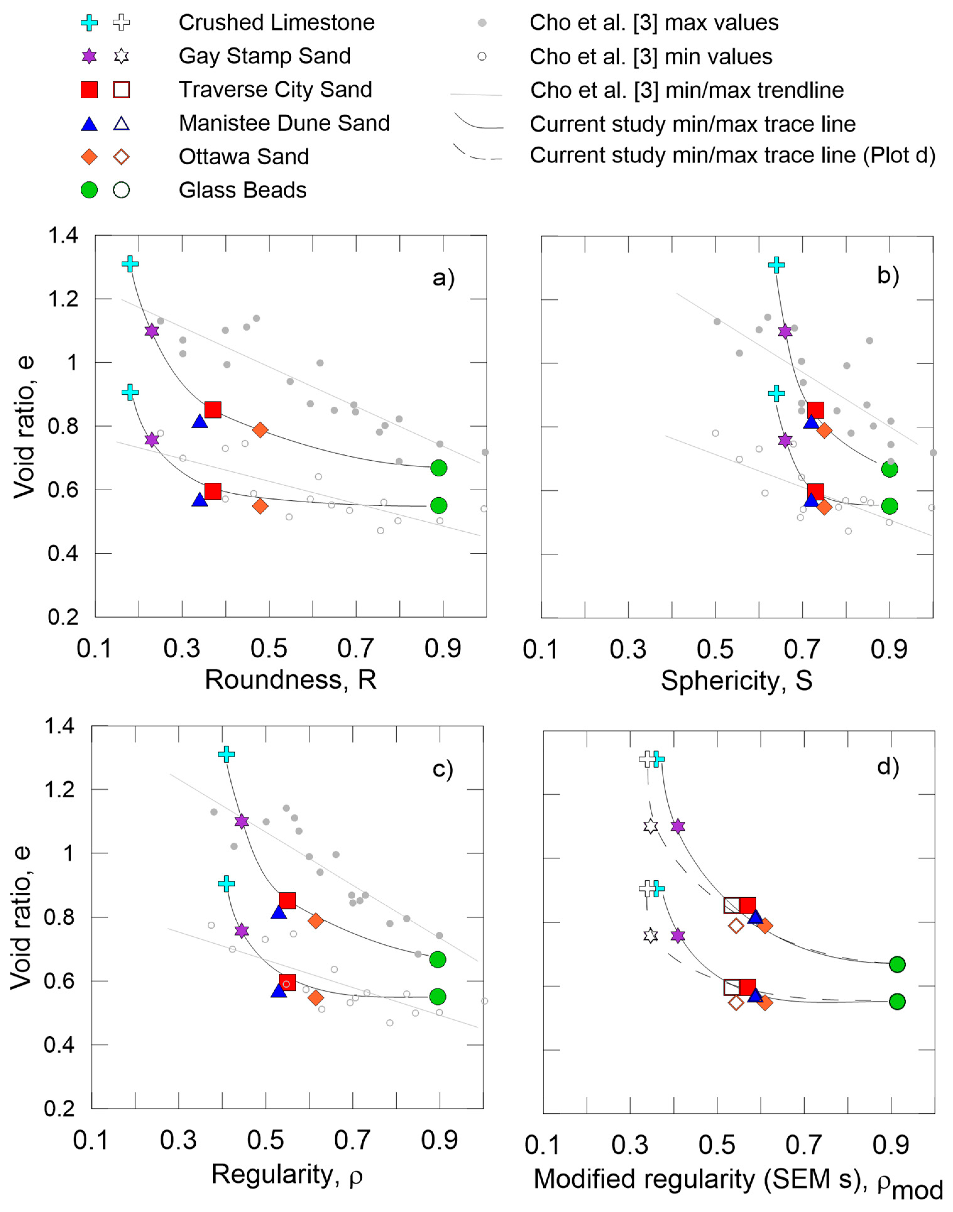
4.1. Maximum and Minimum Void Ratio

Muszynski [29] detailed the approach utilized for obtaining the maximum and minimum void ratios (e_max and e_min) of the specimens. The simplified method uses a mold reminiscent of a smaller version of a Proctor mold. The maximum density is found by tapping the sides of the mold to densify the specimen, while avoiding particle segregation by size. The minimum density is determined by slowly pouring sand into the mold through a funnel. This laboratory work was well suited to this simplified method for determining e_max and e_min, as the graded 30–40 (0.425 to 0.6 mm) sands did not include a large available specimen mass. Additionally, several tests could be conducted to arrive at an average for e_max and e_min, allowing for an evaluation of the consistency of the results.

The specific gravity of solids, G_s, was obtained for each graded soil using a helium pycnometer or the conventional ASTM D 854 method. The helium pycnometer method yields values comparable to those of the conventional ASTM D 854 method [30].

The average results of the maximum and minimum (limit) void ratios for the specimens are shown in

Table 6. Laboratory results of six 30–40-graded specimens.

Soil Name a	R b	S b	ρ	s c	ρmod-sem c	s e	ρmod-om e	Gs	emax	emin	Ie d	ϕrep deg	q f cc/s
Glass beads	0.89 WR g	0.90	0.90	0.95	0.91	0.95	0.91	2.47	0.668	0.551	0.117	23.0	28.6
Crushed limestone	0.18 A	0.64	0.41	0.25	0.36	0.20	0.34	2.76	1.31	0.906	0.404	36.7	11.6
Manistee dune sand	0.34 SA	0.72	0.53	0.71	0.59	0.70	0.59	2.68	0.818	0.571	0.247	32.6	19.4
Ottawa sand	0.48 SR	0.75	0.62	0.60	0.61	0.40	0.54	2.66	0.789	0.548	0.241	32.3	20.4
Gay stamp sand	0.23 A	0.66	0.45	0.33	0.41	0.15	0.35	2.90	1.10	0.758	0.342	35.4	17.1
Traverse City sand	0.37 SR	0.73	0.55	0.62	0.57	0.50	0.53	2.69	0.852	0.595	0.257	32.8	20.1

^a Soil graded to include particles passing a #30 sieve (0.600 mm) and retained on a #40 sieve (0.475 mm). ^b “Large scale visual estimate” of R and S as presented by Muszynski and Vitton [1]. ^c Smoothness, s, determined using visual methods on SEM images described in this document. ^d I_e = void ratio interval = e_max − e_min. ^e Using optical microscope s estimates. ^f 1 cm diameter funnel. ^g Qualitative labels as per Table 1.

. The results of the limit void ratios against R, S, ρ, and ρ_mod (evaluated using individual s parameters from both the optical microscope and SEM) are shown graphically in Figure 9a–d, respectively. It should be noted that the connecting lines (between data points) are not considered to be trendlines, but rather “traces”, which are intended to aid the reader in understanding the progression of the results, and to better follow the results with the eye.

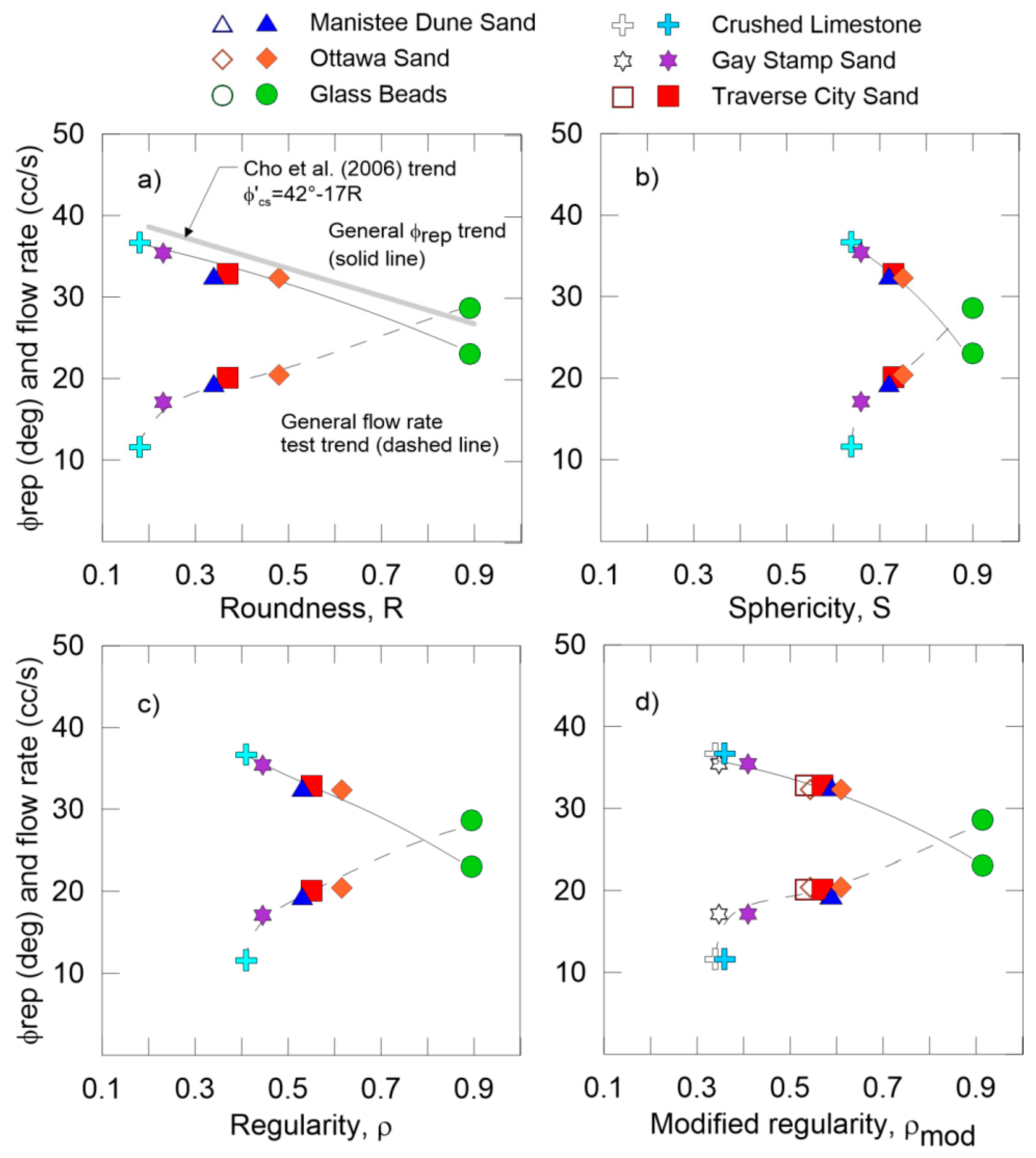
4.2. Angle of Repose

The angle of repose, ϕ_rep, is a useful concept in indirectly obtaining the strength characteristics of a sand. The ϕ_rep is an indicator of the angle of internal friction corresponding to the large strain friction angle/constant volume friction angle, ϕ_cv [20,21,31], or critical state friction angle, ϕ_cs [3]. Therefore, it is regarded as reasonable to consider the critical state friction angle, constant volume friction angle, and angle of repose as being approximately equivalent (i.e., ϕ_cs~ϕ_cv~ϕ_rep).

Santamarina and Cho [32] evaluated ϕ_cs by observing the angle of a submerged specimen after slowly tipping the specimen in a glass cylinder. This procedure worked for the clean specimens considered. In the current study, a tabletop angle of repose test approach was used to obtain an indication of the critical state/constant volume friction angle. Since active ASTM standards do not currently exist for determining ϕ_rep, the following technique was used: First, a piece of thick glass was placed on top of the level surface of a heavy table that was not subject to vibration. Next, static electricity was removed from the glass surface using a dryer sheet. The specimen was then poured through a funnel onto the flat, smooth glass surface. Very small amounts of material were then carefully removed from the toe of the sand specimen using stiff cardboard to create the steepest angle possible. Finally, several measurements were recorded using angle guides. The results of the measurements for ϕ_rep were averaged and are shown in Table 6, as well as against the particle shape parameters R, S, ρ, and ρ_mod (using individual s values obtained from both the optical microscope and SEM) in Figure 10a–d, respectively.

Figure 10a also includes the Cho et al. [3] relationship between the critical state friction angle (ϕ_cs) as a function of roundness, R (ϕ_cs = 42 − 17R). The specimens used to arrive at that well-known and recognized relationship generally had coefficients of uniformity (C_u) less than 2.5. In contrast, the specimens in this study were more narrowly graded than those specimens used in [3], and they had C_u values near unity, perhaps explaining some of the differences in the results. The graphical depiction of the relationship by Cho et al. [3] is located just above the results of the current study in Figure 10a.

4.3. Flow Rate through a Funnel

Dickin [33] demonstrated that the flow rate through a funnel is related to the general particle shape of a dry specimen. For our work, in a similar approach to [33], a recorded mass of each sand specimen was sent through a funnel with a tip diameter of 1 cm. The amount of time required for the sand to pass through was recorded, and several trials were completed to evaluate consistency and establish an average result. The mass measurements were then converted to volume using the G_s for each specimen, and the flow rate q was computed in cm³ of sand per second. The average results of the flow rate testing are shown in Table 6, and also against the particle shape parameters in Figure 10. Once again, trace lines—rather than trendlines—are included in this figure to aid in viewing the progression of the results (ϕ_rep or q against the particle shape parameter noted on the abscissa).

5. Discussion

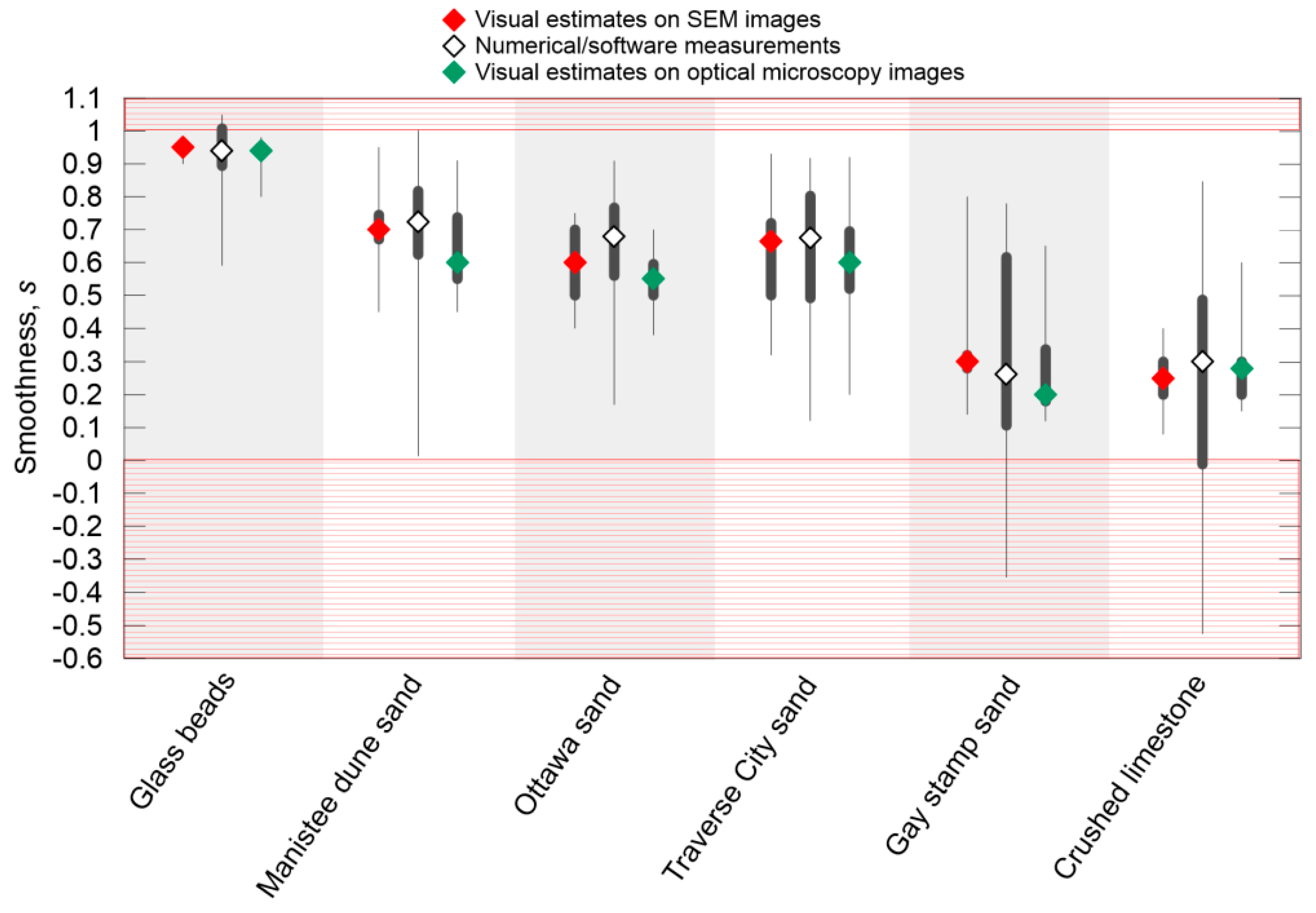
5.1. Smoothness Measurements

Evaluating the surface smoothness of sands requires a different approach to thinking than that of evaluating the shape parameters R and S. With s, the observer must examine the particles on a much smaller scale, which requires additional care.

The use of images obtained with SEM technology offers some advantages over evaluation using optical images, in that SEM makes use of electrons rather than the light viewed by the observer. With SEM images, some of the variables that an observer would notice are bypassed, as the SEM images provide a grayscale image that is purely representative of the distance that the electrons traveled, whereas optical images contain reflections, shading, and other complicating factors. Table 5 shows the comparison of the s estimates using the visual classification method on individual SEM images and the visual classification method on a sample of representative particles as observed through an optical microscope, along with the visual evaluation of individual particles depicted in optical microscopy images, and finally numerical results. As this table shows, the consistency between the methods is reasonable in most cases—particularly for either the mean or the median of the estimated s values.

All things considered, and even though the process of smoothness evaluation is rather objectively complex, the human eye/brain is apparently able to estimate s in a reasonably useful and repeatable manner using the visual estimate approach on either the SEM or optical images. Additionally, a 10× hand lens has shown to be effective in allowing the observer to collect usable s estimates, whether quantitative or qualitative [2]. The numerical analyses conducted suggest that the visual estimates are sufficient in terms of accuracy and consistency.

The options for evaluating s are many, including (from most to least involved) scanning electron microscopy, optical microscopy, visual estimates with a low-cost USB microscope, or, in limited cases of larger particles, a visual estimate using a hand lens. In evaluating the various methods for estimating and/or measuring s, we offer a summary of considerations of the apparent benefits and drawbacks of each approach in

Table 7. Advantages and disadvantages of various smoothness evaluation techniques.

Approach for Evaluating Smoothness (s)	Advantages	Disadvantages
Visual evaluation using SEM images; individual particle evaluation	Humans able to visual detect major s differences with relative repeatability Able to evaluate numerous individual particles for greater confidence	Obtaining SEM images may be costly Setup time (obtaining images, etc.) is potentially lengthy Subtle differences in s become rather subjective Although the evaluation time is not excessive, it still requires ~5 min per 40 particles, for example
Visual evaluation using optical microscopy images; individual particle evaluation	Humans able to visual detect major s differences with relative repeatability Able to evaluate numerous individual particles for greater confidence Optical image capture is relatively cost-effective and becoming more cost-effective rapidly Image capture using recent low-cost USB microscopes is time-effective	Obtaining optical images may be time=consuming using traditional optical microscopy methods Subtle differences in s become rather subjective Although the evaluation time is not excessive, it still requires ~5 min per 40 particles, for example Mindset of evaluation is slightly different based on whether a translucent mineral is evaluated as compared with an opaque mineral
Visual using optical images; specimens’ s evaluated collectively	Humans able to visually detect major s differences with relative repeatability Optical image capture is relatively cost-effective and becoming more cost-effective rapidly Image capture using recent low-cost USB microscopes is time-effective Evaluation time is very rapid (~5 s) once images have been obtained	Obtaining optical images may be time-consuming using traditional optical microscopy methods Subtle differences in s become rather subjective
Visual using a hand lens; specimens’ s evaluated collectively	Humans able to visually detect general s differences with relative repeatability May be performed in the field with a hand lens Evaluation time is very rapid (~5 s)	Works best for quartz-based sands (where “milkiness”, frost and/or surface gloss, etc., may be more clearly observed)

.

5.2. Laboratory Index Testing

Figure 9 and Figure 10 show that e_max and e_min, ϕ_rep, and q are all strongly dependent on particle shape. The results show general trends similar to those observed in the literature [3,4,32,34]. However, some apparent anomalies can be observed. The Manistee dune sand, with R = 0.34, had an I_e of 0.247, as compared with the Traverse City sand, which had R = 0.37 and a greater I_e of 0.257. This relationship should have been reversed if the usual observation of a less rounded sand with an increased I_e were to hold true.

Another observation was made with respect to the results of q for the Ottawa sand, Manistee dune sand, and Traverse City sand. Although these three sands have substantially different average R values, their results for q appear very similar. It seems that the results should be much different, particularly for the Ottawa sand versus the Manistee dune sand and Traverse City sand. When s is included in the particle shape description in the form of ρ_mod, with s visually evaluated based on either SEM images or optical microscopy, values for q closer to those expected are observed. For example, although the Ottawa sand has a greater value of R than the Manistee dune sand and the Traverse City sand, when s is considered, ρ_mod is relatively similar for all three soils (SEM- or optical-microscope-based evaluations of s). This may help explain the similarity in q. And when analyzing I_e for these three soils, the expected trend is observed when ρ_mod (SEM) is used as the particle shape indicator. The trend for I_e observed when the optical microscope is used to estimate s is not as clear-cut, although the results for ρ_mod (optical microscope) indicate a similarity in that parameter between the Manistee dune sand, Ottawa sand, and Traverse City sand.

With decreasing R, the limit void ratios generally increase, as does the range between e_max and e_min, I_e (Figure 9). The trend appears reversed, or ambiguous, between the Ottawa sand, Manistee dune sand, and Traverse City sand. This observation appears to support the idea that R alone does not solely influence the behavior of these graded sands. Upon closer examination through the use of the parameter s, we determined that the Manistee dune sand was actually slightly smoother than the Traverse City sand, while the Ottawa sand was slightly rougher than the Traverse City sand. As ρ_mod was considered for these soils, the observed trend in limit void ratio seemed more predictable, particularly for the SEM-image-based s estimates.

Also included—and superimposed on Figure 9a–c—are the results of the limit void ratios found by Cho et al. [3], mainly for the purpose of comparing the minimum void ratios. For example, the “mid-range” of R values (R = 0.4 to 0.7) for the maximum limit void ratio appeared to be rather low—perhaps closer to what would be expected for the minimum limit void ratio values (see Figure 9a–c). The highly angular crushed limestone specimen also had both minimum and maximum limit void ratio values that were seemingly out of range when compared to those of [3]. These apparent differences in limit void ratio results are not necessarily alarming, because the C_u was substantially different between the specimens of the current study and those of the previous study by Cho et al. [3]. The majority of the other results for limit void ratios in the current study are generally consistent with those of [3], despite the difference in C_u.

The ϕ_rep value increased with a decrease in R, as expected (Figure 10). The relationship found by Cho et al. [3] between ϕ_cs and R (ϕ_cs = 42 − 17R) was located just above the results of this current study. Once again, this appears to be of little surprise, as the C_u values in this study were substantially less than those used to develop the relationship by [3].

Although roundness leads to a strong correlation with certain behaviors of sands, the role of smoothness also plays a measurable and observable role and should be considered to make a more complete description of the overall particle shape. This is particularly the case for the results of the limit void ratios, where including the contribution of s serves to clarify the limit void ratio results. Including the s parameter in matters concerning trends of flow rate and ϕ_rep (e.g., Figure 10c,d) seems to lead to a less dramatic difference in the appearance of the trends. Even so, evaluation of s provides a more complete description of particle shape and potential behavior. However, we should note that other recent studies (e.g., Tessari et al. [2]) have shown measurably different results in various sand specimens’ behaviors, with s isolated as the only variable in play.

Today, with the advent of low-cost USB microscopes, in conjunction with smartphones, obtaining high-quality images in an instant and while onsite is easier than ever. Failing that, examination of a sand specimen onsite with the use of a hand lens continues to be a viable option (particularly if qualitative estimates are suitable at a minimum). At the least, a rapid visual examination of the particle-scale parameters, including s, helps to better understand the likely behavior of the ground and/or avoid certain problems that may surface.

One potential problem arises when a geotechnical engineer works or consults on a site in an unfamiliar location, possibly containing sand with drastically different parameters, and, in turn, exhibits unexpected behavior under loading. An example is as follows: Suppose a soil engineer is familiar with an area containing, perhaps, rounded and rather smooth sands. The soil engineer may have a good feel for what the results of a standard penetration test (SPT) should mean for a given soil deposit with which they are acquainted, and for how past structures have performed in their area. The same engineer perhaps then accepts an assignment working on a development underlain by a vast expanse of stamp sand. The stamp sands are probably more angular and rough-surfaced. Under these conditions, the SPT values could be interpreted erroneously, and foundation settlement predictions could be well off the mark. A cursory observation, at a minimum, of the shape and smoothness parameters may be adequate to give the engineer additional insight about the likely behavior of the soil under various loading conditions. An indication of this behavior in terms of the penetration resistance of a sand with a given relative density and particle shape was described by Muszynski [35] using a miniature cone penetration test.

6. Conclusions

In this article, a new computer-based approach to improve the characterization of surface smoothness of sand particles is proposed. The research described here also presents significant advancements in the evaluation and understanding of the macroscale response of coarse-grained soils. The advancements in low-cost digital microscopy and the development of a new numerical routine for quantifying surface texture are particularly noteworthy. These advancements not only make the method more accessible to a wider audience but also improve the accuracy of predictions related to the behavior of sands. However, at this time, the technique is limited to the range of particle sizes described in this paper, although future research efforts will focus on expanding the technique to encompass natural sands. The key advancements are as follows:

This study introduces a novel smoothness estimation approach utilizing open-source software, which is a more objective numerical analysis measurement technique. This technique enables the rapid and economic quantification of smoothness, which can aid practitioners and academics in their understanding of the macroscale response of coarse-grained soils.

The technique utilizes the recent availability of ultralow-cost digital microscopes, which bypass the need for an expensive traditional optical microscope or specialized laboratory equipment. This advancement extends the viability of the method to a wider audience, who may not have access to expensive and specialized equipment. The study further demonstrates the effectiveness of said microscopes in capturing the surface features of sand particles at a quality level approximately equivalent to that of more traditional methods.

This research shows that human perception is apparently able to estimate smoothness in a reasonably useful and repeatable manner using the visual estimate approach on either the SEM or optical images. However, the sample size of persons was limited and may not be representative of a larger population group.

This paper presents a new numerical routine, using open-source software, designed to quantify surface smoothness and intended to be useful in verifying the results of the visual evaluation approaches.

This study also demonstrates measurable differences in the behaviors of the sands versus predictions when only roundness and sphericity were considered. When smoothness was included in the predictions, the results for the flow rate through a fixed orifice, limit void ratios, interval void ratios, and frictional angles aligned better with expectations and apparent trends.

References

1. Muszynski, M.R.; Vitton, S.J. Particle Shape Estimates of Uniform Sands; Visual and Automated Methods Comparison. J. Mater. Civ. Eng. 2012, 24, 194–206. [Google Scholar] [CrossRef]
2. Tessari, A.; Muszynski, M.R.; Colletti, J. Surface Smoothness Evaluation of Etched and Unaltered Sand Specimens with Mechanical Behavior Assessment. Geotech. Test. J. 2018, 42, 20170261. [Google Scholar] [CrossRef]
3. Cho, G.C.; Dodds, J.S.; Santamarina, J.C. Particle Shape Effects On Packing Density, Stiffness and Strength: Natural and Crushed Sands. J. Geotech. Geoenviron. Eng. 2006, 132, 591–602. [Google Scholar] [CrossRef]
4. Holubec, I.; D’Appolonia, E. Effect of Particle Shape on the Engineering Properties of Granular Soils. In Evaluation of Relative Density and Its Role in Geotechnical Projects Involving Cohesionless Soils; ASTM STP 523; American Society for Testing and Materials: West Conshohocken, PA, USA, 1973; pp. 304–318. [Google Scholar]
5. Youd, T.L. Factors Controlling Maximum and Minimum Densities of Sands. Evaluation of Relative Density and Its Role in Geotechnical Projects Involving Cohesionless Soils; ASTM STP 523; American Society for Testing and Materials: West Conshohocken, PA, USA, 1973; pp. 98–112. [Google Scholar]
6. Powers, M.C. A New Roundness Scale for Sedimentary Particles. J. Sediment. Petrol. 1953, 23, 117–119. [Google Scholar] [CrossRef]
7. Krumbein, W.C. Measurement and Geological Significance of Shape and Roundness of Sedimentary Particles. J. Sediment. Petrol. 1941, 11, 64–72. [Google Scholar] [CrossRef]
8. Wadell, H. Volume, Shape, and Roundness of Rock Particles. J. Geol. 1932, 40, 443–451. [Google Scholar] [CrossRef]
9. Krumbein, W.C.; Sloss, L.L. Stratigraphy and Sedimentation, 2nd ed.; W.H. Freeman and Co.: San Francisco, CA, USA, 1963; p. 660. [Google Scholar]
10. Muszynski, M.R.; Vitton, S.J. Discussion of “Particle Roundness and Sphericity from Images of Assemblies by Chart Estimates and Computer Methods” by: Roman D. Hryciw, Junxing Zheng, and Kristen Shetler. J. Geotech. Geoenviron. Eng. 2017, 143, 07017024. [Google Scholar] [CrossRef]
11. Hryciw, R.; Zheng, J.; Shetler, K. Particle Roundness and Sphericity from Images of Assemblies by Chart Estimates and Computer Methods. J. Geotech. Geoenviron. Eng. 2016, 142, 04016038. [Google Scholar] [CrossRef]
12. Folk, R.L. Student Operator Error in Determination of Roundness, Sphericity and Grain Size. J. Sediment. Petrol. 1955, 25, 297–301. [Google Scholar]
13. Rodriguez, J.; Johansson, J.; Edeskär, T. Particle shape determination by two-dimensional image analysis in geotechnical engineering. In Proceedings of the Nordic Geotechnical Meeting, Copenhagen, Denmark, 9–12 May 2012; pp. 207–218. [Google Scholar]
14. Altuhafi, F.; Coop, M.; Georgiannou, V. Effect of particle shape on the mechanical behavior of natural sands. J. Geotech. Geoenviron. Eng. 2016, 142, 04016071. [Google Scholar] [CrossRef]
15. Masad, E.A. Aggregate Imaging System (AIMS) Basics and Applications; Report 5-1707-01-1, Project 5-1707-01; Texas Transportation Institute and the Federal Highway Administration: College Station, TX, USA, 2004.
16. Santamarina, C.; Cascante, G. Effect of Surface Roughness on Wave Propogation Parameters. Geotechnique 1998, 48, 129–137. [Google Scholar] [CrossRef]
17. Payan, M.; Khoshghalb, A.; Senetakis, K.; Khalili, N. Effect of particle shape and validity of Gmax models for sand: A critical review and a new expression. Comput. Geotech. 2016, 72, 28–41. [Google Scholar] [CrossRef]
18. Alshibli, K.A.; Alsaleh, M.I. Characterizing Surface Roughness and Shape of Sands Using Digital Microscopy. J. Comput. Civ. Eng. 2004, 18, 36–45. [Google Scholar] [CrossRef]
19. Leon, E.; Gassman, S.L.; Talwani, P. Accounting for Soil Aging when Assessing Liquefaction Potential. J. Geotech. Geoenviron. Eng. 2006, 132, 363–377. [Google Scholar] [CrossRef]
20. Cornforth, D.H. Prediction of Drained Strength of Sands from Relative Density Measurements. ASTM Spec. Tech. Publ. (STP) 1973, 523, 281–303. [Google Scholar]
21. Holtz, R.D.; Kovacs, W.D. An Introduction to Geotechnical Engineering; Prentice-Hall, Inc.: Englewood Cliffs, NJ, USA, 1981; p. 517. [Google Scholar]
22. Kramer, S.L. Geotechnical Earthquake Engineering; Pearson: New York, NY, USA, 1996. [Google Scholar]
23. Olson, S.M. Liquefaction Analysis of Level and Sloping Ground Using Field Case Histories and Penetration Resistance. Ph.D. Dissertation, University of Illinois at Urbana-Champaign, Urbana, IL, USA, 2001. [Google Scholar]
24. Konrad, J.M. Sand state from cone penetrometer tests: A framework considering grain crushing stress. Géotechnique 1998, 48, 201–215. [Google Scholar] [CrossRef]
25. Poulos, S.J.; Castro, G.; France, J.W. Liquefaction evaluation procedure. J. Geotech. Eng. 1985, 111, 772–792. [Google Scholar] [CrossRef]
26. Hardin, B.O. Crushing of soil particles. J. Geotech. Eng. 1985, 111, 1177–1192. [Google Scholar] [CrossRef]
27. Santamarina, J.C.; Cho, G.C. Soil behavior: The Role of Particle Shape. In Advances in Geotechnical Engineering: The Skempton Conference; Thomas Telford: London, UK, 2004; pp. 604–617. [Google Scholar]
28. Kulhawy, F.H.; Mayne, P.W. Manual on Estimating Soil Properties for Foundation Design; No. EPRI-EL-6800; Electric Power Research Inst.: Palo Alto, CA, USA, 1990. [Google Scholar]
29. Muszynski, M.R. Determination of Maximum and Minimum Densities of Poorly Graded Sands Using a Simplified Method. Geotech. Test. J. 2006, 29, 263–272. [Google Scholar]
30. Vitton, S.J.; Lehman, M.A.; Van Dam, T.J. Automated Soil Particle Specific Gravity Analysis Using Bulk Flow and Helium Pycnometry, Nondestructive and Automated Testing for Soil and Rock Properties; ASTM STP 1350; Marr, W.A., Fairhurst, C.E., Eds.; American Society for Testing and Materials: West Conshohocken, PA, USA, 1998. [Google Scholar]
31. Mesri, G.; Hayat, T.M. The Coefficient of Earth Pressure at Rest. Can. Geotech. J. 1993, 30, 647–666. [Google Scholar] [CrossRef]
32. Santamarina, J.C.; Cho, G.C. Determination of Critical State Parameters in Sandy Soils—Simple Procedure. Geotech. Test. J. 2001, 24, 185–192. [Google Scholar]
33. Dickin, E.A. Influence of Grain Shape and Size upon the Limiting Porosities of Sands. In Evaluation of Relative Density and Its Role in Geotechnical Projects Involving Cohesionless Soils; ASTM STP 523; American Society for Testing and Materials: West Conshohocken, PA, USA, 1973; pp. 113–120. [Google Scholar]
34. Burmister, D.M. The Importance and Practical Use of Relative Density in Soil Mechanics. ASTM Proc. 1948, 48, 1249–1268. [Google Scholar]
35. Muszynski, M.R. Effects of Particle Shape and Gradation on Miniature DCP Tests in Sand. Geotech. Test. J. 2008, 31, 531–539. [Google Scholar] [CrossRef]
Figure 1. SEM images of selected particles showing proposed smoothness s values (modified from reference [2]).
Geotechnics 03 00046 g001
Figure 2. Sand specimens at 50× magnification using the SEM: (a) glass beads; (b) crushed limestone; (c) Manistee dune sand; (d) Ottawa sand; (e) Gay stamp sand; (f) Traverse City sand.
Geotechnics 03 00046 g002
Figure 3. Sand specimens at 150× magnification using the SEM: (a) glass beads; (b) crushed limestone; (c) Manistee dune sand; (d) Ottawa sand; (e) Gay stamp sand; (f) Traverse City sand.
Geotechnics 03 00046 g003
Figure 4. Sand specimens at 500× magnification using the SEM: (a) glass beads; (b) crushed limestone; (c) Manistee dune sand; (d) Ottawa sand; (e) Gay stamp sand; (f) Traverse City sand.
Geotechnics 03 00046 g004
Figure 5. Sand specimens at 1500× magnification using the SEM: (a) glass beads; (b) crushed limestone; (c) Manistee dune sand; (d) Ottawa sand; (e) Gay stamp sand; (f) Traverse City sand.
Geotechnics 03 00046 g005
Figure 6. Optical microscope images (30×) of the 30–40 specimens considered with inlaid low-cost USB microscope images/thumbnails: (a) glass beads; (b) crushed limestone; (c) Manistee dune sand; (d) Ottawa sand; (e) Gay stamp sand; (f) Traverse City sand.
Geotechnics 03 00046 g006
Figure 7. Examples of raw USB microscope images of (a) a crushed limestone sample and (b) Traverse City sand, showing differences in smoothness features using the appearance of the particles.
Geotechnics 03 00046 g007
Figure 8. Bar-and-whisker plot of smoothness, s, for visual estimates and numerical measurements.
Geotechnics 03 00046 g008
Figure 9. Relationship between limit void ratios for the 30–40-graded specimens: (a) roundness, R; (b) sphericity, S; (c) regularity, ρ; (d) modified regularity with ρmod-om using the s results from optical microscopy and ρmod-sem using the s results from SEM; note that in plot d the open symbols correspond to the optical-microscopy-derived s values, and the solid symbols to the SEM-derived s values.
Geotechnics 03 00046 g009
Figure 10. Relationship between angle of repose, ϕrep, and flow rate through a funnel against: (a) roundness, R; (b) sphericity, S; (c) regularity, ρ; (d) modified regularity, ρmod. Note that plot d includes the optical-microscope-derived s values (open symbols) and the SEM-derived s values (solid symbols) for the 30/40-graded specimens [3].
Geotechnics 03 00046 g010