Review of Methods to Solve Desiccation Cracks in Clayey Soils


Division of Civil & Building Services Engineering (CBSE), London South Bank University (LSBU), London SE1 0AA, UK
Geotechnics 2023, 3(3), 808-828; https://doi.org/10.3390/geotechnics3030044
Submission received: 2 June 2023
/
Revised: 3 August 2023
/
Accepted: 8 August 2023
/
Published: 10 August 2023
Abstract
:This paper reviews numerical methods used to simulate desiccation cracks in clayey soils. It examines five numerical approaches: Finite Element (FEM), Lattice Boltzmann (LBM), Discrete Element (DEM), Cellular Automaton (CAM), and Phase Field (PFM) Methods. The paper presents a simplified description of the methods, including their basic numerical formulations. Several factors such as the multiphase nature of soils, heterogeneity, nonlinearities, coupling, scales of analysis, and computational aspects are discussed. The review highlights the characteristics, strengths, and limitations of each method. FEM shows a good capacity to deal with the thermo-hydromechanical behavior of clays when drying that complement well with the ability of DEM to deal with particle interactions as well as LBM, PFM, and CAM to deal with complex crack patterns. The article concludes by reviewing the integration of multiple numerical methods to enhance the simulation of desiccation cracks in clayey soils and proposing what is the best option to continue improving the study of this problem.
1. Introduction
After more than a century of research from experimental [1,2,3,4,5,6,7,8,9,10,11,12,13,14,15,16,17], theoretical [18,19,20,21,22], and numerical points of view [23,24,25,26,27,28,29], desiccation cracks in clayey soils is still an open research field due to their complexity. It has two very different components, desiccation, which is the loss of water due to water evaporation, and cracking, a failure produced when reaching the strength of the soil. The first is a thermo-hydromechanical (THM) problem [30] and the second is a fracture mechanics (FM) problem [31]. This topic is important because when clayey soil desiccates and cracks, its properties change, becoming more permeable and less strong against loads.
Simulating desiccation cracks in clayey soils is a complex task due to several reasons.
Firstly, clayey soils are multiphase media composed of soil particles, and pores that contain only air, only water, or water and air, depending on if the condition is dry, saturated, or unsaturated. Secondly, clayey soils exhibit coupled nonlinear THM behavior. As moisture content decreases, the soil undergoes significant volume changes due to the suction generated in the soil matrix, resulting in shrinkage first and cracking when the soil strength is reached. This nonlinear behavior requires advanced constitutive models and numerical techniques to accurately capture the soil’s response to environmental contour conditions [32]. The coupling of multiple physical processes, including fluid flow, heat transfer, and deformation is accounted for by incorporating temperature-dependent and moisture-dependent properties. Additionally, constitutive relationships are employed to couple moisture content and mechanical behavior. Thermal expansion coefficients and thermal conductivity should be considered as functions of mechanical strain/stress to account for the coupling between temperature and deformation. Thirdly, the behavior of desiccation cracks is influenced by various factors such as soil composition, mineralogy, pore structure, and initial moisture content. The inherent variability and uncertainties associated with these factors make it difficult to predict crack formation and propagation accurately [33,34,35]. Fourthly, simulating desiccation cracks often requires considering different scenarios, from laboratory specimens to field-scale applications. Accounting for scale effects and capturing the heterogeneity of soil properties is crucial for realistic simulations [36]. Finally, simulating desiccation cracks in clayey soils requires computationally intensive simulations due to the need to solve complex nonlinear coupled equations and handle large deformation and long-term drying processes.
This problem involves several interconnected physical processes in a portion of a multiphase soil system that is in mechanical equilibrium. The shrinkage that takes place as moisture is lost is governed by the principle of balance, known as Richards’ equation, and the generalized Darcy’s law. At the same time, there will be a distribution of temperature governed by the heat balance equation and Fourier’s law. Mechanical deformation arises from shrinkage, exhibiting elastic and plastic behavior described by the THM constitutive model [30].
In the pores of the soil, there are physical processes that occur during the desiccation and cracking. The air dissolution in water is governed by Henry’s law, and the diffusion of air in water is governed by Fick’s law, with water molecules moving from areas of high moisture content to low moisture content. Additionally, heat transfer occurs under effects such as Soret’s thermal diffusion of water vapors in the air because of pressure gradients produced by temperature gradients [37,38,39], vapor effusion, and Stefan’s flow [40]. Fortunately, in many cases, they can be neglected and continue capturing the main mechanisms that govern the desiccation and cracking processes. Thus, they are not necessarily needed in a formulation and a numerical model.
At the beginning of the desiccation, the soil is a saturated fluid slurry, but with time, the condition turns to compacted unsaturated soil. For this reason, the degree of saturation must be included in the formulation and simulation by using, for example, a simplified Van Genuchten’s formula [41] or more complex variations that include the effect of temperature. To accurately model the mechanical behavior of clayey soils during desiccation, THM constitutive equations are necessary. These equations define the relationship between stress and strain and capture the material’s response when suction and temperature change. The simplest stress–strain relationship is the generalized isotropic linear elastic model commonly known as Hooke’s law, which characterizes stress–strain behavior in the linear elastic range. Even if the soil’s mechanical behavior is considered elastic, the equation must include the effect of the temperature and suction to couple the thermal, hydraulic, and mechanical processes. More sophisticated models are nonlinear, viscoelastic, or plasticity, such as bilinear, Mohr–Coulomb models, and many others.
To simulate the initiation and propagation of cracks, Griffith’s criterion (tensile strength controls the initiation of the cracks) or linear elastic fracture mechanics (LEFM) equations are commonly used due to their simplicity. LEFM principles and its rules determine the critical crack length and assess crack propagation. Incorporating LEFM principles allows for the analysis of crack formation and growth during desiccation. The numerical simulation of crack propagation is in particular a very challenging problem in the context of the Finite Element Method (FEM). For this reason, several approaches to simulate the cracking process have been proposed apart from the FEM. Lattice Boltzmann (LBM), Discrete Element (DEM), Cellular Automaton (CAM), and Phase Field (PFM) methods are all alternatives to the FEM that can be used to effectively simulate the desiccation cracks in clayey soils and cracks in other problems.
These numerical techniques enable the solution of complex equations and the simulation of desiccation cracks in clayey soils. Boundary conditions, initial conditions, and appropriate numerical algorithms also play a crucial role in accurately capturing the behavior of desiccation cracks. Figure 1 shows a laboratory test made on a cylindrical sample to study the problem of desiccation cracks in clayey soils under controlled conditions. A whole cycle of drying, wetting, flooding, drying, and cracking demonstrated that flooding produces more cracks and wetting modifies suction profiles. Even when this problem is usually studied as a desiccation problem, the first semi-cycle in Figure 1, wetting and flooding are part of the problem and significantly affect the cracking process. Today, the research community is working mainly on semi-cycles of desiccation. To fully understand this problem, the whole cycle must be understood.
2. Methods to Simulate Desiccation Cracks in Clayey Soils
In the attempt of simulating desiccation cracks in soils, researchers have used physical-based approaches and non-physical-based approaches. In this section, five of the most effective methods to resolve this problem are commented on in terms of the main characteristics, strengths, and limitations. The strengths of these methods are presented in Table 1.
2.1. The Finite Element Method (FEM)
FEM [23,24,26,32,34] and its variant Extended Finite Element Method (XFEM) [42] have been extensively used for simulating desiccation cracks in clayey soils at a macroscale level and can also be applied at micro- and mesoscale levels. Researchers have employed FEM to study moisture diffusion, shrinkage, and cracking behavior during drying.
FEM resolves classic transient continuum mechanics’ partial differential equations that describe the phenomenon. FEM has been successful in capturing the complex behavior of desiccation cracks since it can deal with complex geometries and heterogeneity. It can map the distribution of stress in the soil mass locating the areas of concentration of stresses that produce cracks. FEM deals well with coupling the thermo-hydromechanical physical processes that the problem includes. The accuracy of this method relies on the appropriate implementation of constitutive models and boundary conditions.
The limitations FEM has shown are mesh dependency, making it challenging to capture intricate crack patterns. Additionally, it has shown difficulties in accurately predicting crack propagation without explicit crack geometry modeling. FEM and the other methods presented here neglect soil–structure and soil–atmosphere interaction (Figure 2), which can significantly influence crack formation and behavior. Finally, calibrating constitutive models to accurately represent soil behavior is always a challenge when using FEM and any other numerical approximation. These limitations drive the need for specialized techniques and alternative numerical methods to overcome these challenges and improve the accuracy of simulations.
During the desiccation process, the three phases of the soil interact in general thermally, hydraulically, and mechanically. Once the contour conditions in suction, temperature, and displacements are set, and if the soil–structure and soil–atmosphere interactions are neglected, the main equations that define the THM problem of desiccation in clayey soils are the governing equations and constitutive equations from continuum mechanics, respectively.
In the next section, the formulation for the desiccation cracks problem using FEM is presented. All the details of this formulation, including numerical examples, can be found in [32].
2.1.1. Equilibrium Equation (Cauchy Equation of Motion)
If no dynamic effects are considered, the equilibrium equation of the soil matrix is as follows:
Equation (1) is an elliptic partial differential equation where is the total stress tensor, and is the average density of the multiphase medium (soil, water, or air). The vector is the gravity vector.
2.1.2. Balance Equation (Continuity Equation also Known as Richards’ Equation)
Equation (2) is a parabolic partial differential equation that represents the balance of water in the pores of the soil. In an unsaturated porous medium (the general case that includes the saturated case, and the dry case, ), the water mass balance equation is written as follows:
In Equation (2), is the water density, is Darcy’s velocity vector, is time, is the porosity of the soil, and is the degree of saturation of water in the soil pores.
2.1.3. Conservation of Energy Equation (First Law of Thermodynamics)
If thermal effects are considered, the first law of thermodynamics establishes the need for the heat transfer equation in the soil. Equation (3) is a parabolic partial differential equation:
In Equation (3), is the density of the soil, is the specific heat capacity, is the temperature, is the heat transfer rate, and is the thermal conductivity (could be scalar for isotropic permeability or tensorial for anisotropic permeability).
2.1.4. Stress–Strain Thermos-Mechanical Constitutive Law
For the most general case of unsaturated soils, the effective stress tensor () is:
In Equation (4), is the total stress tensor. The air and water pressure are, respectively, and , is a parameter that depends on the degree of saturation, the stress history and the soil’s fabric and are the identity tensor.
In this formulation, the matrix suction and the net mean stress define the effective stress tensor through Equation (4):
The net stress and the suction are:
The general strain–stress relation must be written in differential form, because of the nonlinearity of the material behavior.
For the most general THM case, is a tangent matrix in function of the strain, , temperature, , and suction, . Equation (7) establishes the coupling between temperature, suction, and mechanical effects.
The deformations are calculated by the addition of a component due to the net stress plus a component due to the suction plus a component due to temperature. Equation (8) considers, then, the additive deformation hypothesis:
In Equation (8), the parameter is the volumetric modulus and is the shear modulus of the soil matrix; the parameter is the volumetric modulus due to changes in suction; the parameter is the volumetric modulus due to temperature changes. These parameters must be established depending on the constitutive model chosen (linear elastic, non-linear elastic, viscoelastic, plastic, etc.); the factor is a fourth-order compliance tensor and are second-order tensors.
The net stress increments can be obtained from (8):
In Equation (9), is the tangent stiffness tensor.
2.1.5. Generalized Darcy’s Law for Unsaturated Soils and Permeability Tensor
The generalized Darcy’s law for unsaturated soils is:
In Equation (10), is the velocity of Darcy’s vector; is the gradient of the suction; is a permeability tensor that changes with water saturation degree, , porosity, , and temperature, ; is the gravity vector and is the water density. The permeability tensor, , can be isotropic or anisotropic.
2.1.6. Water Retention Curve
The van Genuchten function [13] is usually adopted in this formulation to relate changes between the degree of saturation and the suction, :
where, is a material parameter and is the air entry value for the initial porosity , adopted as the reference value. Function considers the changes of porosity during desiccation and its effect in the water retention curve using a parameter, . For non-deformable soils, , because porosity is constant.
2.1.7. Fourier’s Law
This is the constitutive law for the thermal problem.
In Equation (12), is the heat transfer rate and is the thermal conductivity.
2.1.8. Hydro-Mechanical Formulation to Resolve Desiccation Cracks in Clayey Soils
As it was stated in previous sections, desiccation cracks in clayey soils are in general a THM problem. However, since the experimental programs are made under controlled conditions, it is usually chosen to work under isothermal conditions to simplify the study of the process [32,34]. Under these assumptions, the numerical simulations can be HM since the temperature will remain constant during the whole process. Under HM conditions, the problem is resolved by FEM resulting in the system of Equation (13) in what is known as a u-p formulation. This assumption simplifies the problem considerably since Equations (3) and (12) are not needed and Equations (7)–(9) are less complex.
In Equation (13), u are the displacements and p is the suction.
The factors in Equation (13) are:
2.2. Lattice Boltzmann Method (LBM)
LBM was introduced to simulate fluid flow for the first time in 1986 [43]. It was used to study fluid flow and fluid–solid interaction in [44,45]. LBM was used for dealing with several other problems like melting and solidification [46], gas transport into rocks [47], hydraulics fracturing [48], multiphase flow through micro- and macropores [49], fracture and flow [50], and finally, drying [51] and desiccation cracks [52].
LBM enables the consideration of pore-scale processes during drying. The fluid domain is discretized into a lattice structure, with each lattice node representing a small volume or pore. Instead of solving the governing equations at a continuum level, LBM simulates the behavior of individual fluid particles, represented by lattice cells or lattice Boltzmann particles, that move and interact within the lattice. By explicitly representing the individual fluid particles and their interactions, LBM allows for the consideration of various pore-scale processes during dryings, such as capillary effects, evaporation, fluid–solid interactions, and convective flows.
LBM employs a simplified kinetic model to describe the motion of fluid particles. These particles propagate along discrete lattice directions and undergo collisions with neighboring particles, leading to the redistribution of mass, momentum, and energy. The particle interactions at the pore scale directly influence the macroscopic behavior of the fluid.
LBM provides a means to couple pore-scale simulations with larger-scale models, such as FEM, to capture the interactions between the microscopic and macroscopic phenomena. This enables the integration of pore-scale information into continuum-based simulations and improves the accuracy of predictions at larger scales.
LBM provides insights into the fundamental mechanisms of crack formation, but its computational cost can be relatively high due to the need for fine spatial resolution. LBM can solve physical equations of balance and equilibrium. LBM is based on the Boltzmann equation that is derived from the principles of the conservation of mass, momentum, and energy, hence, a physical-based model.
The limitations of the LBM are that the accurate representation of soil behavior in LBM requires proper material characterization, which can be challenging due to the complexity of clayey soil slurry behavior during desiccation. Modeling crack propagation may need additional techniques, as the inherent lattice structure of LBM may not directly capture the process. Additionally, LBM primarily focuses on fluid flow, potentially overlooking some soil mechanics aspects when the soil acquires consistency, such as the mechanical behavior of the soil matrix, which influences crack initiation and propagation.
2.2.1. Formulation of LBM
LBM can be considered as a variant of the Finite Difference Method [53] since it generates a grid (lattice) where the fluid flow is simulated. However, its roots are statistical rather than deterministic [54].
The method calculates the probability of fictitious particles, that compose the material being modeled, being located at a particular point on a lattice as a function of time. It is executed by performing two algorithms. Algorithm 1 models the streaming of particles traveling from one lattice node to connected neighbors. Algorithm 2 mimics their collision (Figure 3). The response of the particles to collision and the lattice used determine the model behavior.
2.2.2. A Multi-Material Multiple-Relaxation-Time LBM
LBM models the statistical mechanics of many particles under collision [49,50]. In the formulation presented in [50], the objective of the method is to simulate the evolution of a single-particle-distribution function of statistical mechanics, . Where, is the position of the particle, is the velocity of the particle, and is time. The function, , is the probability of finding a particle at the position, , velocity, , at time, .
In this method, the mass and momentum conservation equations for an isotropic material can be written as Equations (21) and (22):
where, is the ghost density; is the momentum in the three directions of the space; and are the bulk and deviatoric components of the momentum tensor; is the mean stress and is the deviatoric stress. and bulk and shear coefficients of viscosity.
In three dimensions, the stress is defined as in Equations (23) and (24):
In LBM, the connection between the probability distribution function, , of particles and the conservation equations (mass and momentum) is established through the streaming and collision steps.
Streaming step: After collision, the particles’ are streamed to neighboring lattice nodes according to their velocities. This step ensures the propagation of information through the fluid domain. By streaming particles, the macroscopic properties, such as density and velocity, are advected throughout the simulation domain.
Collision step: In this step, particles collide with each other locally, leading to the redistribution of particle velocities. The collision process obeys conservation laws, such as mass and momentum conservation. During collision, the equilibrium of is determined based on local fluid properties, like density and velocity, at a given lattice point. The equilibrium of represents the that the system would tend toward if no collisions occurred. The key point is that the macroscopic properties of the fluid, such as density and velocity, are related to the moments (summations) of the . The zeroth moment corresponds to the particle density (mass conservation), and the first moment corresponds to the momentum density (momentum conservation). By tracking and updating the function through the collision and streaming steps, the LBM indirectly solves the conservation equations.
2.3. Phase Field Method (PFM)
PFM appeared in 1992 and it was used as an effective tool for simulating desiccation cracks in clayey soils from micro- to mesoscale levels. PFM describes the evolution of a system with multiple phases and has been applied to represent the degree of saturation or water content in the soil [55,56,57,58].
PFM provides a continuous representation of crack formation and propagation, enabling the study of complex crack patterns. However, the computational cost associated with PFM is high. PFM is a mathematical framework that can be used to solve physical equations of balance and equilibrium, so, it is a physical-based method.
The limitations of PFM are the difficulty in accurately calibrating the model parameters to represent the specific behavior of clayey soils. The constitutive relations and material properties used in the PFM may need to be carefully tuned to capture the unique characteristics of clayey soils, such as their complex moisture retention and swelling-shrinkage behavior. Additionally, the PFM tends to smooth out crack features due to its diffuse interface representation of cracks, potentially overlooking small-scale crack details. The cracks change the contour conditions of the problem; since the method treats the cracks with continuous functions, the method cannot update the contour conditions.
2.3.1. General Phase Field for Fracture Model
In this section, the formulation for the desiccation problem from [55] is resumed to their basic elements. The necessary variational approach for cracks was proposed initially by the authors of [59], the phase field implementation is due to [60] and an overview can be found in [61]. In this method, crack surfaces are represented by a surface density function in terms of an auxiliary phase field. Such an approach is known to be thermodynamically consistent and recent works have illustrated its potential to be predictive for a wide range of fracture problems. Phase field for fracture models have succeeded in capturing complex crack patterns, including branching and coalescence in two and three dimensions [62,63,64,65,66].
In Figure 4, the solid is a three-dimensional continuum where the main unknown variables are the displacement field, u, and the phase field, . The contour conditions are the usual Dirichlet boundary and Neumann boundary conditions.
The formulation is presented for infinitesimal deformations in Equation (25):
The total energy in the system is equal to the summation of the external and internal energy as shown in Equation (26):
In a mechanical process, the internal energy is given by Equation (27):
where the elastic energy density is given by Equation (28):
where and are the Lame’s elastic constants. Once a crack is produced in the crack set , the total energy can be expressed as in Equation (29):
is the energy associated with the fracture at , which is in function of the fracture toughness as expressed in Equation (30):
The method requires an explicit surface tracking algorithm and a method to handle the discontinuities. The surface integral is approximated by a volume integral in Equation (31):
is the approximation to the energy released during the cracking process and is the crack-density function.
For the definition of the crack-density function, , Allen–Cahn approximation to the crack surface is used, assuming a smooth transition from d = 1 along the crack set to d = 0 away from the crack set.
In Equation (32), is the local dissipation function and is a regularization parameter carrying units of length.
The system can be resolved by minimizing the total energy, Equation (33):
2.3.2. Govern and Constitutive Equations
The continuum mechanics problem is expressed by the equation of equilibrium and the contour conditions, Equations (34)–(37):
The constitutive laws are, Equations (38) and (39):
where is the degraded stress tensor, is the thermodynamic conjugate to , is the interfacial coefficient, and is often referred to the mobility in keeping with general Allen–Cahn phase field models.
2.4. Discrete Element Method (DEM)
DEM has been used to simulate the behavior of granular materials and clayey soils. DEM considers individual particles and their interactions, enabling the simulation of crack formation during drying. DEM has proven effective in capturing the deformation and interaction between soil particles during drying, but its applicability to large-scale problems can be limited due to high computational costs [67,68,69,70].
While the DEM can accurately simulate the behavior of granular materials, it does not solve the macroscopic equations of balance and equilibrium. Instead, it focuses on capturing the microscale interactions between individual particles and their resulting collective behavior.
The limitations of the DEM method are that, firstly, DEM requires a substantial number of discrete particles to accurately represent the soil structure, making it computationally demanding for large-scale simulations.
Additionally, the accurate characterization of material properties, such as particle-particle interactions, contact forces, and soil–water interaction, can be challenging in clayey soils. The calibration of DEM parameters specific to clayey soils is often complex and time-consuming.
Furthermore, DEM struggles to capture intricate crack patterns and accurately predict crack propagation due to its discrete nature. The method may also overlook important factors, such as the influence of soil matrix behavior and complex moisture redistribution phenomena, which are crucial in desiccation crack simulations.
Thus, while DEM offers valuable insights into the microscale behavior of soil particles, its limitations need careful consideration and validation when simulating desiccation cracks in clayey soils.
DEM Overview
In DEM, the soil is discretized by rigid particles that interact. For example, in [67], the contact behavior is modeled by a system consisting of springs, dashpots, and sliders (Figure 5). The motion of each particle i is governed by the following force and moment balance in Equations (40) and (41):
where and are the translational and rotational accelerations of a particle i, respectively; is the total mass of the particle i; is the acceleration of gravity; is the moment of inertia of the particle i; finally, the force () and moment () acting on particle I can be calculated as follows:
In Equations (42) and (43), and are the normal and shear contact forces at contact c; and are the normal and shear dashpot forces or damping forces; N is the total number of particle i contacts; is the vector from the center of particle i to contact c; and is the mass corresponding with the particle i.
By having particles that represent the soil and particles that represent water, this model [67] can reproduce the desiccation process of a thin layer of clay capturing the characteristic curling behavior during drying.
2.5. Cellular Automaton Method (CAM)
CAM (singular: Cellular Automaton or plural: Cellular Automata) has been employed to simulate the growth and pattern formation of cracks in rocks/clays and is able to work from micro- to macroscale levels [71,72,73,74]. This method uses a grid of cells with different states to represent the crack initiation, propagation, and interaction. CAM offers a simplified representation of crack evolution and is computationally efficient, allowing for the simulation of large-scale crack patterns. The method can simulate heterogeneity in the soil; however, it may lack accuracy in capturing the mechanical behavior of the soil. CAM represents the soil as a 2D or 3D grid of cells and uses rules to simulate the drying process and the resulting stress distribution. The model calculates the evolution of the system over time based on these rules and the initial conditions specified.
This method is what is called a mechanistic method that does not necessarily use physical-based equations to establish its rules. Thus, one limitation of CAM is the challenge of accurately representing the complex behavior of clayey soils within the simplified cellular automata framework. CAM relies on predefined rules and assumptions, which may not fully capture the intricacies of crack formation and propagation in clayey soils. Additionally, the model’s grid-based nature may result in limited spatial resolution, potentially overlooking fine-scale details of crack patterns.
These limitations underscore the need for cautious interpretation and validation of results when applying CAM to simulate desiccation cracks in clayey soils, as well as the potential for combining CAM with other methods to address these shortcomings.
2.5.1. Formulation of CAM
As an example of formulation, the rock discontinuous automaton (RDCA) from [71] is resumed in this section. RDCA includes:
- (1)
- Strong discontinuity;
- (2)
- Tracking a moving crack;
- (3)
- Cellular automaton updating rule;
- (4)
- Yield criteria and crack growth laws.
In Figure 6, this method generates a grid of cells to discretize the continuum. In this example, the grids are squares but the grids can have other shapes (triangles, hexagons, etc.). The elements of the grid are of three types: normal elements (white), elements intersected by a crack (yellow), and elements containing a crack tip (light blue).
- Strong discontinuity
To capture the discontinuous displacement field produced by cracks, Equation (44) was selected [75]:
where represents the total nodal number of the element; is the total nodal number on an element intersected completely by a crack; and are the sets of nodes associated with crack tips 1 and 2 in their influence domain, respectively; , and are the shape functions of the associated node; is the nodal displacements (standard degrees of freedom); and , and are the vectors of the additional degrees of nodal freedom for modeling crack faces and the two crack tips, respectively.
is the Heaviside enrichment function to model the strong discontinuity. It is defined as in Equation (45):
where is the value of the level set function.
- Tracking a moving crack
To track the moving crack, the level set method is used considering the domain is divided into two non-overlapping subdomains, and , that share an interphase as seen in Figure 7a. The level set function is defined [76] as in Equation (46):
An option for the level set function can be simply defined in terms of the signed distance function:
where d is the normal distance from a point x to the interphase .
- Cellular automaton updating rule
In terms of the Cellular Automaton updating rule for continuous problems, they can be elastic, elasto-plastic, elasto-visco plastic, etc. [77]. Discontinuities introduce more complexity. In this method, a cell has nodes , related cell elements and neighbor cell nodes. For every cell, the equilibrium equation is
In Equation (48), is the local stiffness on the cell node, is the incremental degree of freedom, and is the nodal force. The dimension of , , and are dependent on the cell type, i.e., a normal cell or a discontinuous cell. When a cell is intersected by a crack, the cell should be enriched by an enrichment function. The increment nodal force can be obtained from the equation
In Equation (49), is the cell element stiffness. For different element types, such as normal elements, elements with intersecting cracks or elements with crack tips, the cell element stiffness differs.
- Yield criteria and crack growth laws
Different yield criteria can be implemented in this method, Mohr–Coulomb, Drucker–Prager, etc., so, this is suitable for rocks and soils.
For the crack growth, several laws can be used, including maximum circumferential stress, maximum tangential stress, minimum strain energy criteria, etc.
For example, the maximum circumferential stress criterion will be
In Equation (50), is measured with respect to a local polar coordinate system with its origin at the crack tip and is aligned with the direction of the existing crack.
2.5.2. Governing Equations and Local Stiffness Matrix
In Equations (51)–(56), is the Cauchy stress tensor; u is the displacement; b is the body force per unit volume; n is the unit outward normal; and are the prescribed traction and displacement, respectively; is the strain tensor; and C is the Hooke tensor.
3. Integration of Methods to Improve Simulations and Analysis
All the methods in the previous section share limitations that encompass difficulties in accurately characterizing material properties and behavior, representing complex interactions between soil particles, cracks, and fluid flow, and addressing computational demands, particularly for large-scale simulations. Challenges also arise in capturing intricate crack patterns, accurately predicting crack propagation, and incorporating the mechanical behavior of the soil matrix. Furthermore, simulating soil–structure and soil–atmosphere interactions, moisture redistribution, and the microstructure of clayey soils can be challenging. The limitations underscore the need for careful consideration of method selection, calibration of constitutive models, and the exploration of techniques to overcome these challenges and enhance the accuracy and reliability of desiccation crack simulations in clayey soils.
Researchers have explored the combination of multiple numerical methods to simulate the process of desiccation cracks in clayey soils. By combining different methods, they aim to leverage the strengths of each approach to overcome individual limitations and improve the overall accuracy and reliability of the simulations.
For example, the coupling of Scaled Boundary Finite Element Method (SBFEM) with adaptive Phase Field Modeling (PFM) was published in 2019 [78]. This method can model materials that show quasi-brittle fracture properties and reduces the computational effort required by the phase field model. The FEM provides an accurate representation of soil deformation and handles the crack zone by densifying the mesh in the area, while the PFM handles the evolution and propagation of cracks. For hydraulic fracture propagation in rocks, a hydromechanical coupled LBM-DEM model was published in 2018 [79]. This is an interesting combination of physical-based and non-physical based models.
The FEM was coupled with CAM to simulate residual stress of dual-phase steel subjected to laser treatments in a work in 2021 [80]. CAM simulated the microstructure orientation that was after the input for a thermos-mechanical finite element model. This model was able to capture the anisotropy of the material, the dual-phase ferrite–martensite, the temperature sensitivity, and the strain rate influence in the thermos-mechanical behavior. In 2007, three techniques were used to study wave propagation problems. LBM, FEM, and CAM [81] were used in different parts of the geometry of the problem to take advantage of the power of every method.
Hybrid approaches allow for the simultaneous modeling of soil deformation and crack propagation, considering the discrete behavior of soil particles or the fluid flow within the soil matrix. This combination enables capturing both the macroscale behavior of the soil structure and the microscale interactions between particles or fluid.
Additionally, researchers have explored the integration of different methods using a multi-scale double threshold segmentation algorithm [82], methods like free-mesh smoothed particle hydrodynamics method (SPH) [83] and particle discretization scheme finite element method (PDS-FEM) [52]. This involves coupling methods such as FEM, DEM, or LBM at different length scales to capture the behavior of the soil from the microscale to the macroscale. This allows for a more comprehensive understanding of desiccation crack formation and evolution.
While the combination of multiple methods shows promise, it is still an active area of research, and the specific combinations and approaches vary depending on the research objectives and available computational resources.
FEM and CAM are the only methods able to work from micro- to macroscale levels being computationally efficient for large-scale simulation. In the opinion of the author of this paper, FEM is the best method to simulate the desiccation process taking into consideration the complexities of the soil behavior and is a physical-based method.
4. Finite Element and Cellular Automaton Method (FEM-CAM)
After the study of the state of the art, the author arrives to the conclusion that since the problem of desiccation cracks in clayey soils is a multiphysics and multiphase problem (soil matrix + water and air in the pores), it can be resolved using FEM for the THM process and CAM for the cracking problem by developing a FEM-CAM method. The method proposed in this section (for future research) is based on the one proposed by the authors of [80] to simulate residual stress by combining FEM and CAM.
Integration of FEM with CAM to Simulate Desiccation Cracks in Clayey Soils
CAM models the soil as a grid of cells, and each cell can be in different states representing soil moisture content, stress, or cracking. The mathematical formulation of the desiccation crack problem using CAM involves expressing the evolution of moisture content, suction, temperature, and stress, in the soil domain that can be calculated by a THM or HM model resolved by FEM.
In Figure 8, a simplified flow chart shows the coupling between FEM and CAM to solve the desiccation cracks problem. To start the resolution of the problem, the soil domain must be defined by including the geometry, contour conditions, loads, and material properties. FEM is used to discretize the soil domain and then this mesh is used to define the CAM grid and then define the initial conditions. As it was shown in the previous examples of the review, CAM first produces a grid representation of the soil and can establish heterogeneity.
A cracking criterion is defined based on stress thresholds or stress gradients. The criterion determines when a cell transitions from an intact state to a cracked state. For example, a simple criterion could be the crack initiate when the tensile strength is reached in any cell. Once a cell transitions to a cracked state, crack propagation rules determine how cracks propagate to neighboring cells. This can be based on stress redistribution or local crack propagation rules. The direction and extent of crack propagation can be influenced by factors such as stress concentration, crack coalescence, and crack branching.
One the CAM model is updated with the new cracks, the moisture content, suction, stress, temperature, and cracking states are updated at each time step using FEM. The specific equations and constitutive relationships used will depend on the chosen modeling approach and the characteristics of the soil being studied.
Finally, a direct, iterative, or embedded strategy is necessary to couple FEM with CAM. The degree of convergence of every time step will depend on the accuracy needed to resolve specific problems. The final step in the method will be the postprocessing of the results in terms of stresses, strains, humidity, temperature, etc., and should show the final configuration of cracks in the soil.
5. Conclusions
Modeling and simulating desiccation cracks in clayey include cycles of drying, wetting, flooding, and re-drying (Figure 1) that will complicate the formulation and implementation of numerical models in the future even more.
The five methods reviewed in this paper include the Finite Element (FEM), Lattice Boltzmann (LBM), Phase Field (PFM), Discrete Element (DEM), and Cellular Automaton (CAM) Methods, whereby each one has their strengths and limitations when applied to this problem.
FEM captures very well and with consistency the THM desiccation process at a macroscale level and can be applied to micro- and mesoscale levels also. Being based on the continuum mechanics equations makes the method reliable but limited when dealing with complex crack patterns due to the need for complex remeshing that are computationally highly demanding. For example, Ref. [32] presents the simulation of the initiation and propagation of only one crack in 2D, showing a good agreement with laboratory results in terms of water loss and shrinkage. LBM is a good method to simulate the flow of the initial slurry of clayey soil at a mesoscale level but not so well for deformation in connection with the complex THM behavior of clayey soils when it becomes a compacted unsaturated medium. However, Ref. [50] demonstrated the ability of simulating multiple cracks in 2D. PFM is good to simulate micro- and mesoscale continuous cracks, but not so good to capture the THM nature of the process in the soil mass. Again, Ref. [55] has shown the ability to simulate multiple cracks in 2D. DEM is good at simulating the behavior of particles interacting at a microscale level but not so good at capturing the THM nature of the soil behavior and is not a physical-based model. However, Ref. [67] demonstrated that this method can simulate the curling process when clays dry. CAM is good for simulating complex crack patterns at micro-, meso- and macroscale levels, but limited in dealing with the THM desiccation process, which is what makes it ideal to work in combination with FEM. In [71], the ability of this method to simulate cracks in concrete, which can be extrapolated to clays, is demonstrated.
The limitations of these methods working separately, such as introducing heterogeneity, difficulties in accurately characterizing material properties, capturing intricate crack patterns, considering complex soil–fluid, soil–structure, soil–atmosphere interactions, and being computationally highly demanding, highlight the need for further research.
Since the desiccation cracks in clayey soils is a problem well divided into two coupled processes, desiccation and cracking, and considering that FEM simulates the desiccation well, and other methods simulate the cracking process well, their combination seems to be the best option. Then, to address these limitations and improve the simulations, researchers started to explore the combination of different methods. By integrating the strengths of multiple approaches, such as coupling FEM with DEM or LBM, or combining FEM with PFM, it becomes possible to overcome individual limitations and obtain more accurate and reliable simulations. Furthermore, a multi-scale approach, integrating methods at different length scales, allows for a comprehensive understanding of desiccation crack formation and evolution.
The combination of FEM and CAM, presented in Section 4, is a promising alternative since FEM and CAM can capture the process from micro- to macroscale levels and CAM is particularly efficient when computationally intense calculations are needed for large-scale crack pattern simulations. In addition, since they both have the same governing equations and can share the mesh, it seems that they can efficiently work together to resolve desiccation cracks in clayey soils. It is of course difficult to know which method or combination of methods will be the best option to tackle the desiccation crack problem in clayey soils in the coming years, but the aim of this paper is to identify the most promising alternatives based on the research performed up until today.
Funding
This research received no external funding.
Conflicts of Interest
The author declares no conflict of interest.
References
- Kindle, E.M. Some factors affecting the development of mud-cracks. J. Geol. 1917, 25, 135–144. [Google Scholar] [CrossRef] [Green Version]
- Kodikara, J.; Barbour, S.L.; Fredlund, D.G. Desiccation cracking of soil layers. In Unsaturated Soils for Asia; Rahardjo, H., Toll, D.G., Leong, E.C., Eds.; Balkema: Lodon, UK, 2000; pp. 693–698. [Google Scholar]
- Chekhov, V.Y. Modelling cracking stages of saturated soils as they dry and shrink. Eur. J. Soil Sci. 2002, 53, 105–118. [Google Scholar]
- Corte, A.; Higashi, A. Experimental Research on Desiccation Cracks in Soil. Wilmette; DREN: Wilmette, IL, USA, 1964. [Google Scholar]
- Hu, L.B.; Hueckel, T.; Péron, H.; Laloui, L. Modeling Evaporation, Shrinkage and Cracking of Desiccating Soils. In Proceedings of the 12th International Conference of International Association for Computer Methods and Advances in Geomechanics, Goa, India, 1–6 October 2008; pp. 1083–1090. [Google Scholar]
- Lakshmikantha, M.R.; Prat, P.C.; Ledesma, A. Characterization of crack networks in desiccating soils using image analysis techniques. In Numerical Models in Geomechanics X; Pande, G.N., Pietruszczak, S., Eds.; Balkema: London, UK, 2007; pp. 167–176. [Google Scholar]
- Lakshmikantha, M.R.; Prat, P.C.; Ledesma, A. Image analysis for the quantification of a developing crack network on a drying soil. Geotech. Test J. 2009, 32, 505–515. [Google Scholar]
- Lakshmikantha, M.R.; Prat, P.C.; Ledesma, A. Experimental evidence of size-effect in soil cracking. Can. Geotech. J. 2012, 49, 264–284. [Google Scholar] [CrossRef]
- Lakshmikantha, M.R.; Prat, P.C.; Ledesma, A. Evidence of hierarchy in cracking of drying soils. ASCE Geotech. Spec. Publ. 2013, 231, 782–789. [Google Scholar]
- Lau, J.T.K. Desiccation Cracking of Clay Soils. Master’s Thesis, University of Saskatchewan, Saskatoon, SK, Canada, 1987. [Google Scholar]
- Cordero Arias, J.A. Experimental Analysis of Soil Cracking Due to Environmental Conditions. Ph.D. Thesis, UPC-Barcelona Tech, Barcelona, Spain, 2019. [Google Scholar]
- Nahlawi, H.; Kodikara, J. Laboratory experiments on desiccation cracking of thin soil layers. Geotech. Geol. Eng. 2006, 24, 1641–1664. [Google Scholar] [CrossRef]
- Péron, H.; Hueckel, T.; Laloui, L.; Hu, L.B. Fundamentals of desiccation cracking of fine-grained soils: Experimental characterization and mechanisms identification. Can. Geotech. J. 2009, 46, 1177–1201. [Google Scholar] [CrossRef]
- Tang, C.-S.; Shi, B.; Liu, C.; Gao, L.; Inyang, H. Experimental Investigation of the Desiccation Cracking Behavior of Soil Layers during Drying. J. Mater. Civ. Eng. 2011, 23, 873–878. [Google Scholar] [CrossRef]
- Tang, C.-S.; Shi, B.; Liu, C.; Suo, W.-B.; Gao, L. Experimental characterization of shrinkage and desiccation cracking in thin clay layer. Appl. Clay Sci. 2011, 52, 69–77. [Google Scholar] [CrossRef]
- Vogel, H.J.; Hoffmann, H.; Roth, K. Studies of crack dynamics in clay soil. I: Experimental methods, results, and morphological quantification. Geoderma 2005, 125, 203–211. [Google Scholar] [CrossRef]
- Taheri, S.; El-Zein, A. Desiccation cracking of polymer-bentonite mixtures: An experimental investigation. Appl. Clay Sci. 2023, 238, 106945. [Google Scholar] [CrossRef]
- Lachenbruch, A.H. Depth and spacing of tension cracks. J. Geophys. Res. 1961, 66, 4273–4292. [Google Scholar] [CrossRef]
- Morris, P.H.; Graham, J.; Williams, D.J. Cracking in drying soils. Can. Geotech. J. 1992, 29, 263–277. [Google Scholar] [CrossRef]
- Abu-Hejleh, A.; Znidarcic, D. Desiccation theory for soft cohesive soils. J. Geotech. Eng. 1995, 121, 493–502. [Google Scholar] [CrossRef]
- Konrad, J.; Ayad, R. Desiccation of a sensitive clay: Field experimental observations. Can. Geotech. J. 1997, 34, 929–942. [Google Scholar] [CrossRef]
- Konrad, J.; Ayad, R. An idealized framework for the analysis of cohesive soils undergoing desiccation. Can. Geotech. J. 1997, 34, 477–488. [Google Scholar] [CrossRef]
- Lee, F.H.; Lo, K.W.; Lee, S.L. Tension Crack Development in Soils. J. Geotech. Eng. 1988, 114, 915–929. [Google Scholar] [CrossRef]
- Trabelsi, H.; Jamei, M.; Zenzri, H.; Olivella, S. Crack patterns in clayey soils: Experiments and modeling. Int. J. Numer. Anal. Methods Geomech. 2012, 36, 1410–1433. [Google Scholar] [CrossRef]
- Sima, J.; Jiang, M.; Zhou, C. Modeling desiccation cracking in thin clay layer using three-dimensional discrete element method. Proc. Am. Inst. Phys. 2013, 1542, 245–248. [Google Scholar]
- Amarasiri, A.L.; Kodikara, J.; Costa, S. Numerical modelling of desiccation cracking. Int. J. Numer. Anal. Methods Geomech. 2011, 35, 82–96. [Google Scholar] [CrossRef]
- Sánchez, M.; Manzoli, O.L.; Guimarães, L.N. Modeling 3-D desiccation soil crack networks using a mesh fragmentation technique. Comput. Geotech. 2014, 62, 27–39. [Google Scholar] [CrossRef]
- Gui, Y.; Zhao, G.F. Modelling of laboratory soil desiccation cracking using DLSM with a two-phase bond model. Comput. Geotech. 2015, 69, 578–587. [Google Scholar] [CrossRef]
- Guo, L.; Chen, G.; Ding, L.; Zheng, L.; Gao, J. Numerical simulation of full desiccation process of clayey soils using an extended DDA model with soil suction consideration. Comput. Geotech. 2023, 153, 105107. [Google Scholar] [CrossRef]
- Lewis, R.W.; Schrefler, B.A. The Finite Element Method in the Static and Dynamic Deformation and Consolidation of Porous Media, 2nd ed.; Wiley: Hoboken, NJ, USA, 1998. [Google Scholar]
- Griffith, A.A. The phenomenon of rupture and flow in solids. Philos. Trans. R. Soc. Lond. Ser. A 1921, 221, 163–198. [Google Scholar]
- Levatti, H.U. Numerical Solution of Desiccation Cracks in Clayey Soils. In Encyclopedia of Engineering, 1st ed.; Barretta, R., Agarwal, R., Zur, K.K., Ruta, G., Eds.; MDPI: Basel, Switzerland, 2023; Volume 1, pp. 399–421. [Google Scholar]
- Ávila, G. Estudio de la Retracción y el Agrietamiento de Arcillas. Aplicación a la arcilla de Bogotá. Ph.D. Thesis, UPC-Barcelona Tech, Barcelona, Spain, 2005. [Google Scholar]
- Levatti, H.U. Estudio Experimental y Análisis Numérico de la Desecación en Suelos Arcillosos. Ph.D. Thesis, UPC-Barcelona Tech, Barcelona, Spain, 2015. Available online: https://www.tdx.cat/handle/10803/299202#page=1 (accessed on 1 January 2023).
- Lakshmikantha, M.R. Experimental and Theoretical Analysis of Cracking in Drying Soils. Ph.D. Thesis, UPC-BarcelonaTech, Barcelona, Spain, 2009. [Google Scholar]
- Salciarini, D.; Bienen, B.; Tamagnini, C.; Hicks, M.A.; Brinkgreve, R.B.J.; Rohe, A. Incorporating scale effects in shallow footings in a hypoplastic macroelement model. In Proceedings of the 8th European Conference on Numerical, Delft, The Netherlands, 18–20 June 2014. [Google Scholar]
- Platten, J.K. The Soret Effect: A Review of Recent Experimental Results. J. Appl. Mech. 2006, 73, 5–15. [Google Scholar] [CrossRef]
- Ludwig, C. Diffusion zwischen ungleich erwärmten Orten gleich zusammengesetzter Lösung. Sitzungsberichte Akad. Wiss. Math. Naturwissenschaftliche Kl. 1856, 20, 539. [Google Scholar]
- Soret, C. Sur l’état d’équilibre que prend au point de vue de sa concentration une dissolution saline primitivement homogène dont deux parties sont portées à des températures différentes. Ann. Chim. Phys. 1881, 22, 293–297. [Google Scholar]
- Mitrovic, J. Josef Stefan and his evaporation–diffusion tube—The Stefan diffusion problem. Chem. Eng. Sci. 2012, 75, 279–281. [Google Scholar] [CrossRef]
- van Genuchten, M.T. Closed-form equation for predicting the hydraulic conductivity of unsaturated soils. Soil Sci. Soc. Am. J. 1980, 44, 892–898. [Google Scholar] [CrossRef] [Green Version]
- Cheng, W.; Bian, H.; Hattab, M.; Yang, Z. Numerical modelling of desiccation shrinkage and cracking on soils. Eur. J. Environ. Civ. Eng. 2022, 2–21. [Google Scholar] [CrossRef]
- Frisch, U.; Hasslacher, B.; Pomeau, Y. Lattice-gas automata for the Navier-Stokes equation. Phys. Rev. Lett. 1986, 56, 1505–1508. [Google Scholar] [CrossRef] [PubMed] [Green Version]
- Galindo-Torres, S.A. A coupled discrete element size lattice Boltzmann method for the simulation of fluid-solid interaction with particles of general shapes. Comput. Methods Appl. Mech. Eng. 2013, 265, 107–119. [Google Scholar] [CrossRef]
- Chen, S.; Doolen, G.D. Lattice Boltzmann method for fluid flows. Annu. Rev. Fluid Mech. 1998, 30, 329–364. [Google Scholar] [CrossRef] [Green Version]
- Samanta, R.; Chattopadhyay, H.; Guha, C. A review on the application of lattice Boltzmann method for melting and solidification problems. Comput. Mater. Sci. 2022, 206, 111288. [Google Scholar] [CrossRef]
- Yang, J.; Fall, M. Hydro-mechanical modelling of gas transport in clayey host rocks for nuclear waste repositories. Int. J. Rock Mech. Min. Sci. 2021, 148, 104987. [Google Scholar] [CrossRef]
- Mejía Camones, L.A.; Vargas, E.A., Jr.; Velloso, R.Q.; Paulino, G.H. Simulation of hydraulic fracturing processes in rocks by coupling the lattice Boltzmann model and the Par-Paulino-Roesler potential-based cohesive zone model. Int. J. Rock Mech. Min. Sci. 2018, 112, 339–353. [Google Scholar] [CrossRef]
- Kutay, M.E.; Khire, M. Numerical modeling of multiphase flow through micro- and macro-pores of clay landfill caps using Lattice Boltzmann method. In Proceedings of the 7th International Conference on Heat Transfer, Fluid Mechanics, and Thermodynamics, Antalya, Turkey, 19–21 July 2010; Available online: https://repository.up.ac.za/handle/2263/44410 (accessed on 1 March 2023).
- Sikaneta, S. Novel Lattice Boltzmann Methods for Modelling Fracture and Flow. Ph.D. Thesis, Dalhousie University, Halifax, NS, Canada, 2009. Available online: https://www.researchgate.net/publication/241414135_Novel_lattice_Boltzmann_methods_for_modelling_fracture_and_flow (accessed on 2 June 2023).
- Qin, F.; Zhao, J.; Kang, Q.; Derome, D.; Carmeliet, J. Lattice Boltzmann modeling of drying of porous media considering contact angle hysteresis. Transp. Porous Media 2021, 140, 395–420. [Google Scholar] [CrossRef]
- Hirobe, S.; Oguni, K. Coupling analysis of pattern formation in desiccation cracks. Comput. Methods Appl. Mech. Eng. 2016, 307, 470–488. [Google Scholar] [CrossRef]
- Junk, M. A finite difference interpretation of the lattice Boltzmann method. Numer. Methods Partial. Differ. Equ. 2001, 17, 383–402. [Google Scholar] [CrossRef] [Green Version]
- Higuera, F.; Jimenez, J. Boltzmann approach to lattice gas simulations. Europhys. Lett. 1989, 9, 663–668. [Google Scholar] [CrossRef]
- Hu, T.; Guilleminot, J.; Dolbow, J.E. A phase-field model of fracture with frictionless contact and random fracture properties: Application to thin-film fracture and soil desiccation. Comput. Methods Appl. Mech. Eng. 2020, 368, 113106. [Google Scholar] [CrossRef]
- Miehe, C.; Hofacker, M.; Welschinger, F. A phase field model for rate-independent crack propagation: Robust algorithmic implementation based on operator splits. Comput. Methods Appl. Mech. Eng. 2010, 368, 2765–2778. [Google Scholar] [CrossRef]
- Luo, C.; Sanavia, L.; De Lorenzis, L. Phase-field modeling of drying-induced cracks: Choice of coupling and study of homogeneous and localized damage. Comput. Methods Appl. Mech. Eng. 2023, 410, 115962. [Google Scholar] [CrossRef]
- Hun, D.; Yvonnet, J.; Guilleminot, J.; Dadda, A.; Tang, A.; Bornert, M. Desiccation cracking of heterogeneous clayey soil: Experiments, modeling, and simulations. Eng. Fract. Mech. 2021, 258, 108065. [Google Scholar] [CrossRef]
- Francfort, G.; Marigo, J.J. Revisiting brittle fracture as an energy minimization problem. J. Mech. Phys. Solids 1998, 46, 1319–1342. [Google Scholar] [CrossRef]
- Bourdin, B.; Francfort, G.; Marigo, J.J. Numerical experiments in revisited brittle fracture. J. Mech. Phys. Solids 2000, 48, 797–826. [Google Scholar] [CrossRef]
- Bourdin, B.; Francfort, G.A.; Marigo, J.J. The variational approach to fracture. J. Elast. 2008, 91, 5–148. [Google Scholar] [CrossRef]
- Karma, A.; Kessler, D.A.; Levine, H. Phase-field model of mode III dynamic fracture. Phys. Rev. Lett. 2001, 87, 045501. [Google Scholar] [CrossRef] [Green Version]
- Karma, A.; Lobkovsky, A.E. Unsteady crack motion and branching in a phase-field model of brittle fracture. Phys. Rev. Lett. 2004, 93, 245510. [Google Scholar] [CrossRef] [Green Version]
- Henry, H.; Levine, H. Dynamic instabilities of fracture under biaxial strain using a phase field model. Phys. Rev. Lett. 2004, 93, 105504. [Google Scholar] [CrossRef] [Green Version]
- Spatschek, R.; Gugenberger, C.M.; Brener, E. Phase field modeling of fracture and stress-induced phase transitions. Phys. Rev. E 2007, 75 Pt 2, 066111. [Google Scholar] [CrossRef] [PubMed] [Green Version]
- Amor, H.; Marigo, J.J.; Maurini, C. Regularized formulation of the variational brittle fracture with unilateral contact: Numerical experiments. J. Mech. Phys. Solids 2009, 57, 1209–1229. [Google Scholar] [CrossRef]
- Tran, K.M.; Bui, H.H.; Sánchez, M.; Kodikara, J. A DEM approach to study desiccation processes in slurry soils. Comput. Geotech. 2020, 120, 103448. [Google Scholar] [CrossRef]
- Nguyen, N.H.T.; Bui, H.H.; Nguyen, G.D.; Kodikara, J. A cohesive damage-plasticity model for DEM and its application for numerical investigation of soft rock fracture properties. Int. J. Plast. 2017, 98, 175–196. [Google Scholar] [CrossRef]
- Peron, H.; Delenne, J.Y.; Laloui, L.; El Youssoufi, M.S. Discrete element modelling of drying shrinkage and cracking of soils. Comput. Geotech. 2009, 36, 61–69. [Google Scholar] [CrossRef]
- Guo, Y.; Han, C.; Yu, X. Laboratory characterization and discrete element modeling of shrinkage and cracking in clay layer. Can. Geotech. J. 2017, 55, 680–688. [Google Scholar] [CrossRef] [Green Version]
- Pan, P.; Yan, F.; Feng, X. Modeling the cracking process of rocks from continuity to discontinuity using a cellular automaton. Comput. Geosci. 2012, 42, 87–99. [Google Scholar] [CrossRef]
- Pan, P.Z.; Feng, X.T.; Hudson, J.A. Study of failure and scale effects in rocks under uniaxial compression using 3D cellular automata. Int. J. Rock Mech. Min. Sci. 2009, 46, 674–685. [Google Scholar] [CrossRef]
- Gobron, S.; Chiba, N. Crack pattern simulation based on 3D surface cellular automata. Vis. Comput. 2001, 17, 287–309. [Google Scholar] [CrossRef]
- Hosoglu, S. Cellular Automata: An Approach to Wave Propagation and Fracture Mechanics Problems. Ph.D. Thesis, Naval Postgraduate School, Monterey, CA, USA, 2006. [Google Scholar]
- Moës, N.; Dolbow, J.; Belytschko, T. A finite element method for crack growth without remeshing. Int. J. Numer. Methods Eng. 1999, 46, 131–150. [Google Scholar] [CrossRef]
- Osher, S.; Sethian, J.A. Fronts propagating with curvature-dependent speed: Algorithms based on Hamilton–Jacobi formulations. J. Comput. Phys. 1988, 79, 12–49. [Google Scholar] [CrossRef] [Green Version]
- Feng, X.T.; Pan, P.Z.; Zhou, H. Simulation of the rock micro fracturing process under uniaxial compression using an elastoplastic cellular automaton. Int. J. Rock Mech. Min. Sci. 2006, 43, 1091–1108. [Google Scholar] [CrossRef]
- Hirshikesh, A.L.N.; Pramod, R.K.; Annabattula, E.T.; Song, C.; Natarajan, S. Adaptive phase-field modeling of brittle fracture using the scaled boundary finite element method. Comput. Methods Appl. Mech. Eng. 2019, 355, 284–307. [Google Scholar] [CrossRef]
- Chen, Z.; Yang, Z.; Wang, M. Hydro-mechanical coupled mechanisms of hydraulic fracture propagation in rocks with cemented natural fractures. J. Pet. Sci. Eng. 2018, 163, 421–434. [Google Scholar] [CrossRef]
- Liu, S.; Gavrus, A.; Kouadri-Henni, A. Finite element method coupled with a numerical cellular automaton model used to simulate the residual stresses of dual phase DP600 steel Nd: YAG laser welding. In Proceedings of the 23rd Congres Français de Mécanique, Lille, France, 28 August–1 September 2017; Available online: https://hal.science/hal-03465290 (accessed on 2 June 2023).
- Kwon, Y.W.; Hosoglu, S. Application of lattice Boltzmann method, finite element method, and cellular automata and their coupling to wave propagation problems. Comput. Struct. 2007, 86, 663–670. [Google Scholar] [CrossRef]
- Zhou, X.P.; Zhao, Z.; Li, Z. Cracking behaviors and hydraulic properties evaluation based on fractural microstructure models in geomaterials. Int. J. Rock Mech. Min. Sci. 2020, 130, 104304. [Google Scholar] [CrossRef]
- Tran, H.T.; Wang, Y.; Nguyen, G.D.; Kodikara, J.; Sanchez, M.; Bui, H.H. Modelling 3D desiccation cracking in clayey soils using a size dependent SPH computational approach. Comput. Geotech. 2019, 116, 103209. [Google Scholar] [CrossRef]
Figure 1.
Drying, wetting, flooding, and drying 36-day tests on cylindrical clays sample, 80 cm in diameter and 10 cm high, in an environmental chamber. From Dr. Hector U. Levatti—Ph.D. [34].
Figure 1.
Drying, wetting, flooding, and drying 36-day tests on cylindrical clays sample, 80 cm in diameter and 10 cm high, in an environmental chamber. From Dr. Hector U. Levatti—Ph.D. [34].

Figure 2.
Soil–atmosphere and soil–structure (tray) interactions can significantly affect the behavior of the cracks.
Figure 2.
Soil–atmosphere and soil–structure (tray) interactions can significantly affect the behavior of the cracks.

Figure 3.
Lattice Boltzmann method. (a) Algorithm 1—Streaming step. Particles travel to connected neighbors. (b) Algorithm 2—Collision step. Particles travel to lattice node.
Figure 3.
Lattice Boltzmann method. (a) Algorithm 1—Streaming step. Particles travel to connected neighbors. (b) Algorithm 2—Collision step. Particles travel to lattice node.

Figure 4.
(a) An intact solid body with Dirichlet boundary and Neumann boundary . (b) A solid body with a crack represented by the crack set Γ. (c) A solid body with a crack represented by the crack-density function γ (d).
Figure 4.
(a) An intact solid body with Dirichlet boundary and Neumann boundary . (b) A solid body with a crack represented by the crack set Γ. (c) A solid body with a crack represented by the crack-density function γ (d).

Figure 5.
Basic contact model in DEM.

Figure 6.
Cellular automaton model representation.

Figure 7.
(a) Definition of the level set function; (b) Boundary value problem with a crack.
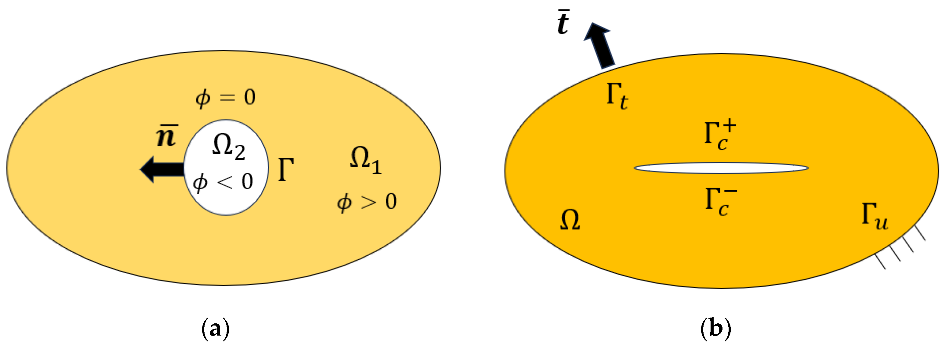
Figure 8.
Simplified flow chart for coupled FEM-CAM method.


Table 1.
Methods that effectively tackle challenges when simulating desiccation cracks in clayey soils, and the scale levels they work into. The methods are classified into non-physical-based (nPb) and physical-based (Pb) methods into columns for every scale level.
Table 1.
Methods that effectively tackle challenges when simulating desiccation cracks in clayey soils, and the scale levels they work into. The methods are classified into non-physical-based (nPb) and physical-based (Pb) methods into columns for every scale level.
| Common Challenges | Non-Physical-Based (nPb) Physical-Based (Pb) | Scale Level | |||||
|---|---|---|---|---|---|---|---|
| Microscale | Mesoscale | Macroscale | |||||
| nPb | Pb | nPb | Pb | nPb | Pb | ||
| Heterogeneity | DEM CAM | FEM | CAM | FEM | CAM | FEM | |
| Multiphase medium | DEM CAM | PFM | CAM | PFM | CAM | FEM | |
| Coupled nonlinear THM problem | DEM CAM | PFM | CAM | LBM PFM | CAM | FEM | |
| Effect of the soil composition, mineralogy, pore structure, initial moisture content | DEM CAM | PFM | CAM | LBM PFM | CAM | FEM | |
| Dealing efficiently with computationally intensive methods at large-scale simulations | CAM | CAM | CAM | ||||
| Large deformations | DEM CAM | PFM | CAM | LBM PFM | CAM | FEM | |
| Capture shrinkage and cracking using advanced constitutive equations | DEM CAM | PFM | CAM | LBM PFM | CAM | FEM | |
| Complex crack patterns | CAM | CAM | CAM | ||||
Disclaimer/Publisher’s Note: The statements, opinions and data contained in all publications are solely those of the individual author(s) and contributor(s) and not of MDPI and/or the editor(s). MDPI and/or the editor(s) disclaim responsibility for any injury to people or property resulting from any ideas, methods, instructions or products referred to in the content. |
© 2023 by the author. Licensee MDPI, Basel, Switzerland. This article is an open access article distributed under the terms and conditions of the Creative Commons Attribution (CC BY) license (https://creativecommons.org/licenses/by/4.0/).
Share and Cite
MDPI and ACS Style
Levatti, H.U. Review of Methods to Solve Desiccation Cracks in Clayey Soils. Geotechnics 2023, 3, 808-828. https://doi.org/10.3390/geotechnics3030044
AMA Style
Levatti HU. Review of Methods to Solve Desiccation Cracks in Clayey Soils. Geotechnics. 2023; 3(3):808-828. https://doi.org/10.3390/geotechnics3030044
Chicago/Turabian StyleLevatti, Hector U. 2023. "Review of Methods to Solve Desiccation Cracks in Clayey Soils" Geotechnics 3, no. 3: 808-828. https://doi.org/10.3390/geotechnics3030044