Tsunami Wave Characteristics from the 1674 Ambon Earthquake Event Based on Landslide Scenarios

Abstract

This study focuses on understanding the historical tsunami events in Eastern Indonesia, specifically the Banda Sea region, by extracting information from the limited and challenging-to-interpret historical records. The oldest detailed account of a tsunami in Indonesia dates back to 1674, documented in the book Waerachtigh Verhael Van de Schlickelijcke Aerdbebinge by Rumphius. The study aims to comprehend the primary source of the tsunami and analyze its characteristics to facilitate future tsunami risk reduction. The methodology includes collecting topography and bathymetry data, conducting landslide scenario analysis, employing a two-layer wave propagation model, and performing spectral analysis. The study utilizes comprehensive datasets, investigates potential landslide scenarios, simulates tsunami propagation, and analyzes frequency characteristics using the fast Fourier transform. The 1674 event yielded a runup height of approximately 50–100 m, whereas this study underestimated the actual runup. To illustrate the tsunami wave along the bay’s coastline, a Hovmöller diagram was employed. By analyzing the Hovmöller diagram, the power spectral density was computed, revealing five prominent period bands: 6.96, 5.16, 4.1, 3.75, and 3.36 min. The integration of these components provides a rigorous approach to understanding tsunami dynamics and enhancing risk assessment and mitigation in the study area.

1. Introduction

One of the regions characterized by highly active and complex tectonic activity is Eastern Indonesia, specifically the Banda Sea [1,2,3,4], as shown in Figure 1. Although the historical record of this area is replete with major destructive earthquakes and tsunamis, most of the significant events in recent times have occurred in western Indonesia. Thus, to better comprehend the tsunami threat in eastern Indonesia, it becomes imperative to extract as much information as possible from the historical record, which often consists of scant and challenging-to-interpret accounts.

The oldest detailed account of a tsunami in Indonesia dates back to Rumphius [5,6]. On 17 February 1674, Ambon and its surrounding islands were rocked by a devastating earthquake. Following the earthquake, a massive tsunami occurred, reaching a run-up height of approximately 100 m. However, this tsunami was only observed on the northern coast of Ambon Island, while other regions experienced only minor tsunamis. The earthquake and ensuing tsunami resulted in more than 2300 fatalities, primarily on the northern shore of Ambon.

The historical documentation of the Ambon earthquake and tsunami on 17 February 1674 can be found in the book Waerachtigh Verhael Van de Schlickelijcke Aerdbebinge, authored by Rumphius [5,6]. An English translation of the book titled The True History of the Terrible Earthquake was published in 1997 [5,6].

The event occurred at around 7:30 p.m. local time, coinciding with the celebration of the Chinese Lunar New Year in Laitimor. In Ambon, the bells in Victoria Castle swung on their own, and individuals standing upright were thrown to the ground as the earth undulated like the sea. Stone structures collapsed, burying up to 80 people. The mountains in Laitimor experienced strong shaking, causing rocks to tumble and the ground to crack open. In Hutumuri, situated near the coast on the eastern side of Laitimor, seawater burst into the air akin to a fountain.

The earthquake was also reported in Hitu. In the Waytome River, on the northern side, the river water spurted up to a height of 6 m. People residing to the north and northwest of Hitu heard a loud sound resembling cannon fire. They observed two long, thin marks in the sky stretching from Luhu to Seith shortly before the earthquake. Less than 15 min after the earthquake, villages between Lima and Hila were obliterated by an enormous wall of seawater. The seawater rose approximately 50 to 60 fathoms (around 90–110 m) and reached the summits of the surrounding hills, resulting in the loss of over 2300 lives.

This extraordinary phenomenon was observed in other areas, albeit with significantly less intensity. Hitu Lama village, located approximately 15 km east of Hila, reported a rise in seawater of only 3 to 5 m, leading to the deaths of 35 individuals. Further east, in Mamala, 40 houses were swept away, but no fatalities were recorded. The settlement of Orien (now known as Ureng), located less than 10 km west of Lima, reported the flooding of land by seawater, although the water did not enter the houses. In Larike, a village in the westernmost part of Hitu, residents noted that the seawater rose less than 1 m at the Rotterdam Redoubt. In the southern and eastern regions of Ambon Island, apart from a few small boats being tossed around, there were few reports of seawater oscillation.

In Luhu, situated in Seram Kecil, the seawater inundated trees, and the dwellings of a company rose to a height of slightly over 5 m. At the northernmost tip of Piru Bay, half of the houses in Tanuno were engulfed by water, yet no fatalities were recorded. Fishermen in Piru Bay noted that the sea remained calm with a noticeable ripple. People from Manipa, Salati, Haruku, Nusa Laut, and Banda Neira Islands reported much lower seawater oscillation compared to the oscillation observed in Hitu and Laitimor. Aftershocks continued for at least 3 months, with the two largest aftershocks occurring on 6 and 10 May. The location of the mentioned place name for this event is indicated in Figure 1.

The source of the tsunami and earthquake remains unknown. Løvholt et al. [7] and Harris and Major [8] have postulated that it may have been triggered by an earthquake south of Ambon and a landslide triggered by an earthquake within Ambon Bay, respectively. However, no further investigations have been undertaken to delve into this event, particularly to ascertain why the extreme run-up was observed solely on the northern coast of Ambon. Therefore, understanding the primary source of the tsunami requires exploring the landslide scenario. Finally, we analyze the characteristics of the tsunami, focusing on wave resonance, to facilitate future planning for tsunami risk reduction.

2. Results and Discussion

2.1. Tsunami Wave Generation and Propagation Results

The tsunami wave generation was simulated using a two-layer model based on three landslide scenarios triggered by the 1764 earthquake. The model incorporated a stratified medium consisting of an upper layer representing seawater with a constant density of ρ₁ (1024 kg/m³) and a lower layer representing fluidized granular material with a density of ρ₂ (2000 kg/m³) and a porosity of φ (0.35). The three landslide scenarios, referred to as scenarios A, B, and C, had volumes of approximately 0.14 km³, 0.2 km³, and 1.12 km³, respectively. The model successfully captured the interactions between tsunami generation and submarine landslides, accurately simulating the dynamics of the tsunami waves. The accuracy of the three scenarios was further validated using measured data, ensuring their reliability and precision.

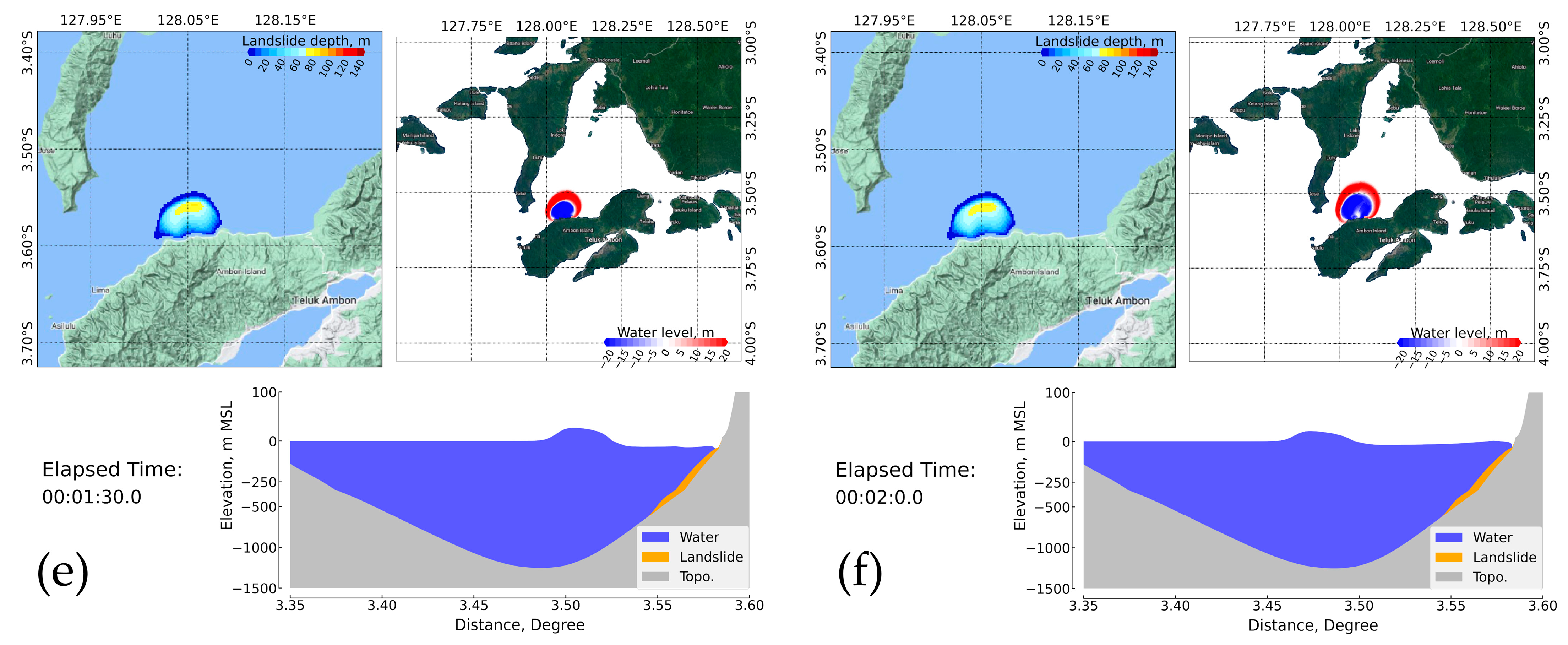
The simulation snapshots of tsunami propagation at different times are shown in Figure 2 at 5, 15, 30, 60, 90, and 120 s after the tsunami was generated by the submarine landslide demonstrated in Scenario C. The simulation animation of tsunami wave propagation demonstrated in the scenario C is presented in Video S1 in the supplementary materials. Single-potential submarine landslide source scenarios were used to demonstrate the generation of the tsunami wave. The single potential submarine landslide generates a solitary wave that propagates northward of the bay. After the landslide stabilizes with a slope of approximately 5 degrees, the maximum amplitudes are approximately 10 m, 25 m, and 50 m for Scenarios A, B, and C, respectively.

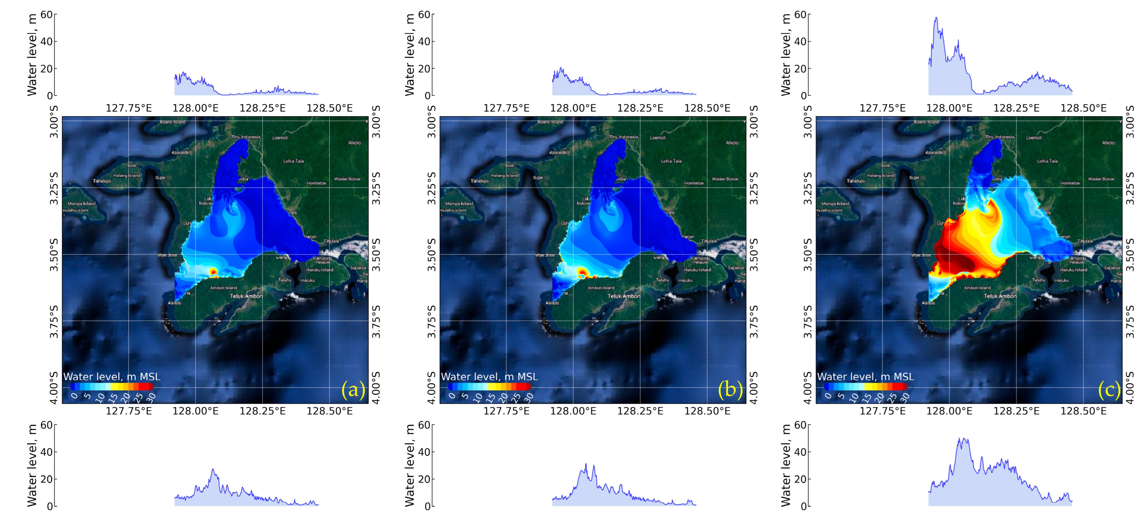
Figure 3 illustrates the maximum water levels resulting from the three landslide scenarios. Figure 3a presents Scenario A, while Figure 3b depicts Scenario B. Scenario C is displayed in Figure 3c. Among the three scenarios, Scenario A exhibits the smallest impact but demonstrates the highest amplitude in the area near the landslide location. In this scenario, the maximum water level on the south shore surpasses that on the north shore. Considering the north shore, the western side experiences a higher maximum water level compared to the eastern side. This difference can be attributed to the deeper bathymetry in the western region, causing the tsunami wave to refract westward. The phenomenon of tsunami wave refraction due to bathymetry has been discussed by Gusman et al. [9].

Scenario B exhibits behavior similar to Scenario A but with higher water level values. In contrast, Scenario C differs from both scenarios in that the maximum water level towards the north is higher than towards the south. The maximum water level in Scenario C surpasses that of both previous scenarios by approximately two times.

Figure 4 illustrates the distribution of inundation depth in the inland area surrounding the shoreline of Piru Bay, as reproduced from the three landslide scenarios. Figure 4a represents Scenario A; Figure 4b depicts Scenario B; and Scenario C is presented in Figure 4c. Among the three scenarios, Scenario A has the smallest impact but exhibits the highest inundation depth in the vicinity of the landslide location. In this scenario, the maximum inundation depth on the south shore reaches approximately 12 m, covering an area of approximately 42.54 km². On the north shore, the western side experiences inundation with a depth of around 1 m, while the eastern side remains unaffected. This variation is attributed to the deeper bathymetry in the western region and the westward refraction of waves.

Scenario B shows similar behavior to Scenario A but with higher inundation depth values. It results in an inundation area of approximately 46.62 km², with a maximum inundation depth of approximately 18 m. In contrast, Scenario C differs from the other two scenarios, with higher inundation depths observed in the north compared to the south. Inundation also occurs in the eastern region, with a depth of approximately 1.5 m. Scenario C reveals a larger inundation area of approximately 139.12 km², with a maximum depth of approximately 32 m.

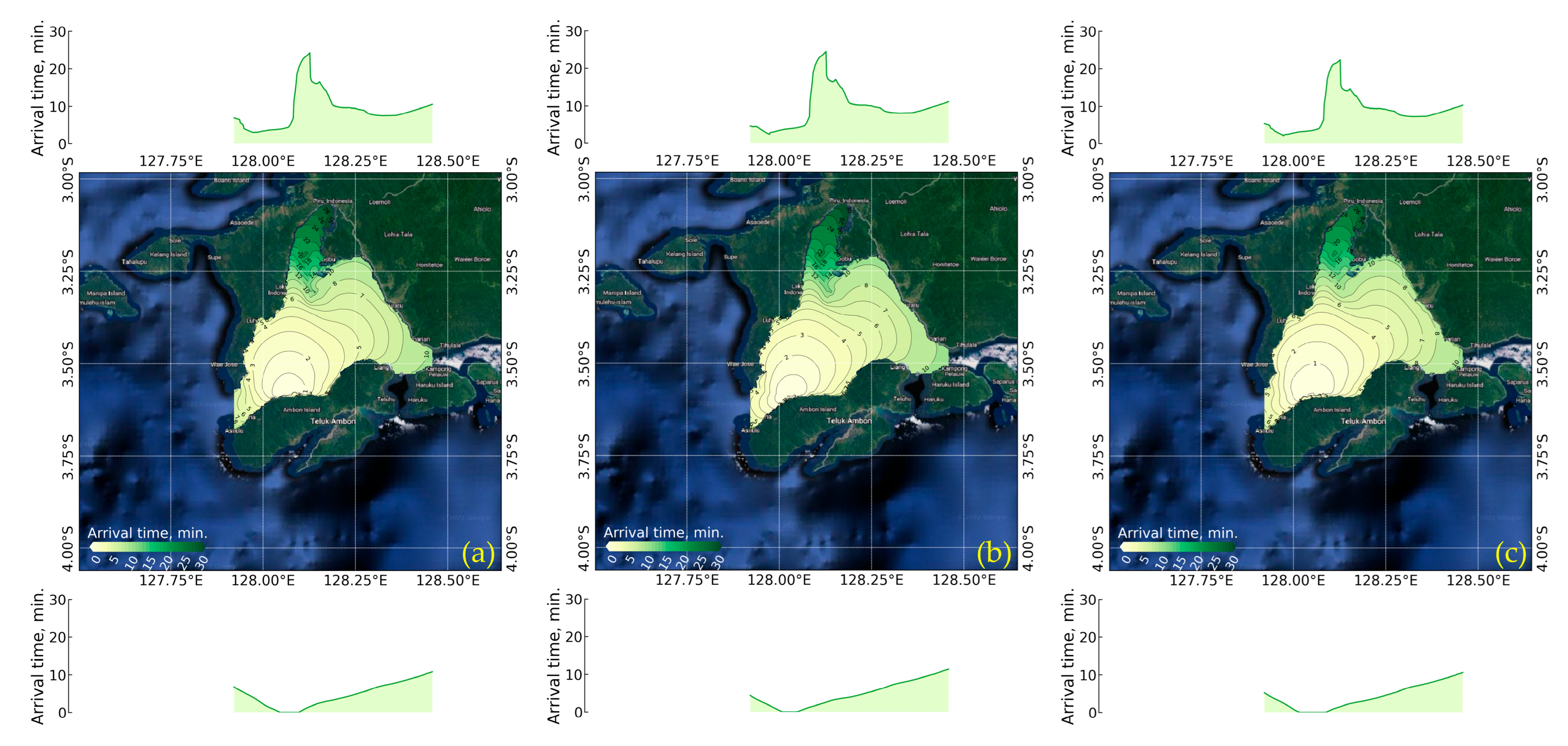
Figure 5 illustrates the tsunami arrival times for the three scenarios: Scenario A (see Figure 5a), Scenario B (see Figure 5b), and Scenario C (see Figure 5c). Each scenario is presented in a separate column. The patterns observed in the three scenarios indicate that the tsunami arrives on the south shore more rapidly than on the north shore. On the north shore, the fastest arrival time across all scenarios is approximately 5 min, while the slowest arrival time is approximately 25 min. In contrast, on the south shore, the fastest tsunami arrival time is approximately 1 min, occurring behind the landslide location. The slowest arrival time on the south shore is approximately 10 min, towards the eastward direction.

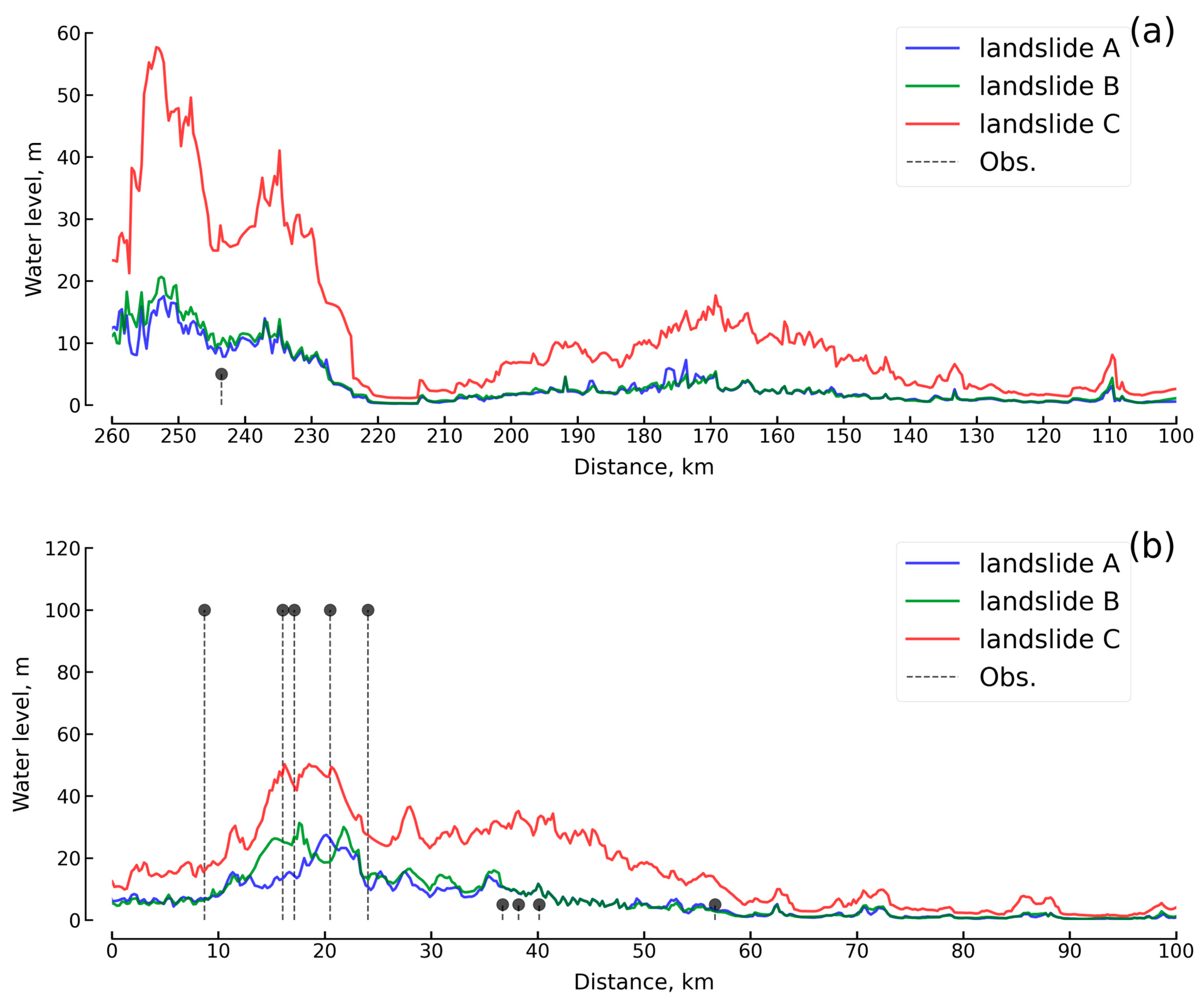
In to Figure 6, the effects of the tsunami resulting from the three landslide scenarios along the coastline of Piru Bay were analyzed over a distance of 260 km, comparing them with the measured data provided by Pranatyo and Cummins [10]. In the southern region spanning 0–30 km, Scenario A exhibited an average tsunami height of approximately 10 m, with a maximum of 20 m at 17 km. In Scenario B, the average height was around 12 m, reaching a maximum of 22 m at 17 km. Scenario C showed significantly higher values, with a tsunami height of approximately 40 m and a maximum of 50 m at 17 km. However, all scenarios underestimated the measured data, which indicated a height of 100 m. Moving along the south shore from 30–70 km, the tsunami heights were approximately 6 m, overestimating the observed data by approximately 5 m. Scenarios A and B closely reproduced the measured tsunami heights, while Scenario C consistently produced higher values, approximately twice the measured height. In the northern region from 70 to 160 km, Scenario A and B had varying tsunami heights of approximately 3 m, with the highest value around 5 m at 120 km. In contrast, Scenario C exhibited greater variability, ranging from approximately 10 m to a peak of 15 m at 120 km. The range from 160 to 260 km indicated that Scenarios A and B closely matched the measured data, both showing a height of 5 m at 240 km. However, Scenario C overestimated the tsunami height by approximately 60 m. Overall, Scenario C had the highest impact compared to Scenarios A and B.

2.2. Spectral Analysis of the Tsunami Wave

The tsunami wave resulting from the two-layer model underwent spectral analysis to examine its frequency characteristics. The analysis employed the fast Fourier transform (FFT) method, utilizing the Numpy library in the Python package. By applying the FFT to the simulated waveform, the spectral amplitudes were obtained as a function of frequency (or period). This analysis allowed for the identification of oscillation patterns and the relationship between the period and amplitude of the tsunami wave. The spectral analysis provided valuable insights into the frequency components and energy distribution within the tsunami wave, contributing to the future risk reduction of tsunamis. We demonstrated scenario C for the spectral analysis, which had the highest impact among the three scenarios.

To understand the pattern of the tsunami wave along the coastline of Piru Bay, we utilized a Hovmöller diagram [11], as shown in Figure 7. The diagram displays the temporal amplitudes of virtual tide gauges spaced at 1 km intervals along the coast, with the horizontal axis representing the distance and the vertical axis representing the time series of the tsunami wave. The diagram revealed a strong tsunami duration from 0 to 40 km and 220 to 260 km, with wave reflections observed at 20 km and 240 km. Another notable phenomenon observed was the presence of edge waves, which are gravity waves trapped by refraction against the coastline. These edge waves were evident at 20 km and 240 km. However, it is important to note that the edge waves were intertwined with shelf resonance, both of which contributed to the long-lasting duration of the tsunami.

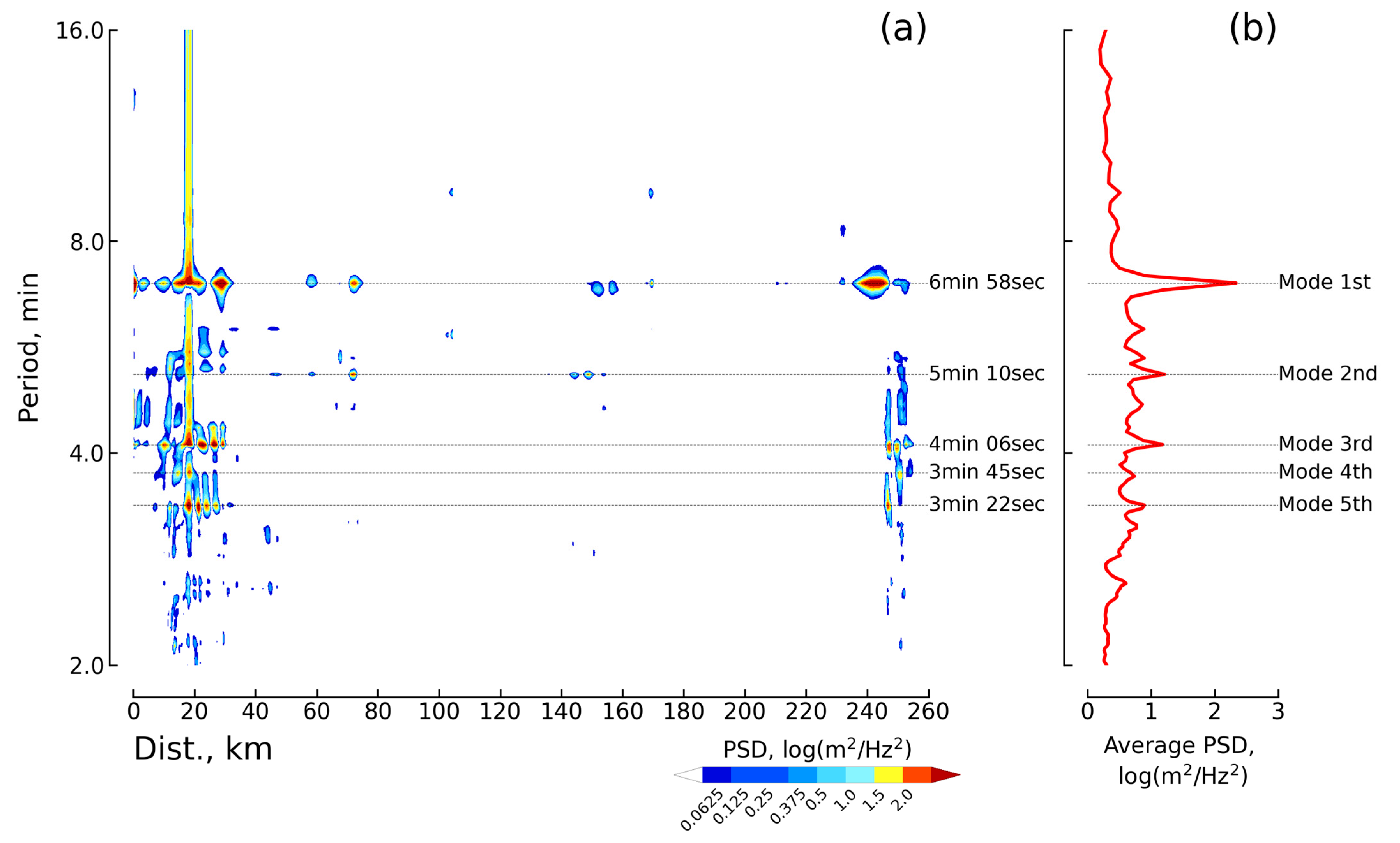
To better understand the contributions from reflection and edge waves, we calculated the power spectral density at each virtual coastal gauge along the coastline, as presented in Figure 8a. The results show that within the main coastline area, the tsunami energy was dominated by five main period bands centered at 6.96, 5.16, 4.1, 3.75, and 3.36 min, as shown in Figure 8b. In the shallow bathymetry area, located in the middle, the energy was concentrated at periods longer than 5 min. The beginning and end of the coastline area exhibited a variation in periods from high frequency to low frequency, representing the deep sea areas of the bay.

Figure 9 (in the first column) displayed the spectral amplitude plots for five representative oscillation modes, providing insights into the tsunami impact around the coastline of Piru Bay. Despite the southwest approach of the tsunami, the energy distribution was relatively even over the bay. The phase plots in Figure 9 (in the second column) reveal that some oscillation modes contained partial standing waves, which did not have well-defined nodes due to irregular coast configurations. Standing waves have the same phase within an antinode and undergo an abrupt 180° phase shift to adjacent antinodes, while partial standing waves show gradual phase variations across the nodes. A uniform phase variation would indicate progressive waves.

The first resonance at 6.96 min corresponds to the fundamental mode of the bay mouth on the western side. The phase plot shows a system of large-scale, partial standing waves on the north and south sides of the bay in the west. The resonance in the area and the partial standing waves were coupled with a 180° phase difference, resulting in minor amplification outside the embayment. At 5.16 min, resonance amplification occurred over the bay with well-defined antinodes on the east sides of the bay. The two antinodes had opposite phases and interacted through the partial standing waves in the area. At 4 min and 6.59 s, resonance oscillation was observed in the south area of the bay, with a node at the coastline and an antinode at the east end of the south. The partial standing waves retreated from the shallow sea and became out of phase over the northern area. This large-scale oscillation became less coherent between the two sides of the insular slope at higher resonance modes.

At 3 min and 45 s, the fundamental mode corresponded to the southern area of the bay. The phase plot shows a system of large-scale partial standing waves on the west side of the bay. Most of the partial standing waves had very small amplitudes, not noticeable in the amplitude plot, but the power could be considerable due to the water depth. The resonance in the partial standing waves was coupled with a 180° phase difference, resulting in minor amplification outside the harbor. The highest detectable resonance mode over the entire shelf occurred at 3 min and 22 s, with four offshore antinodes over the south of the bay and a system of partial standing waves around the area.

The resonance modes help identify areas prone to large oscillations and explain the behavior of the tsunami along the coast of Piru Bay. Figure 10a displays the computed spectral energy and peak period. The spectral energy exceeding 80 cm².s is primarily concentrated along the south coastline and north coastline on the west side of the bay, with some smaller areas in the east. In the middle of the north, there are disruptions in the sea caused by small islands and seamounts.

The peak period of the wave spectrum exhibits variation within the bay, as depicted in Figure 10b. The average peak period falls within the range of approximately 6–8 min, with the highest peak period of around 12 min observed in the east and north regions of the bay, attributable to the shallow sea conditions.

3. Conclusions

In conclusion, the study on the 1674 Ambon earthquake and tsunami in Piru Bay, Eastern Indonesia, has provided significant insights into the characteristics and impacts of past tsunamis in the region. By integrating various data sources and employing advanced modeling techniques, the research has enhanced our understanding of tsunami dynamics in Piru Bay.

The simulation of the tsunami wave generated by submarine landslides in Piru Bay successfully captured the dynamics of wave propagation. The model accurately simulated the interactions between tsunami generation and the three landslide scenarios (A, B, and C), which had varying volumes and resulted in different maximum amplitudes and arrival times. Scenario C was the highest volume of landslides, followed by Scenarios B and A. The accuracy of the two-layer model revealed the overestimation in the small impact area based on the measured data, while the high impact area reproduced the underestimation. The maximum water levels and arrival times varied along the coastline, with Scenario C exhibiting the highest impact and surpassing the measured data. The study provides valuable insights into the behavior of tsunami waves in the bay, contributing to our understanding of their potential impacts and aiding in the development of effective coastal planning and disaster management strategies.

The spectral analysis of the tsunami wave in Piru Bay revealed valuable information about its frequency characteristics, energy distribution, and oscillation patterns. The analysis, performed through the fast Fourier transform method, provided insights into the relationship between the period and amplitude of the wave, contributing to future risk reduction efforts. The Hovmöller diagram demonstrates a strong tsunami duration and the presence of wave reflections and edge waves along the coastline, while the power spectral density analysis highlights dominant period bands and the energy concentration in specific areas. The investigation of resonance modes helped identify regions prone to large oscillations, and the computed spectral energy and peak period analysis shed light on energy concentrations and variability within the bay. These findings enhance our understanding of tsunami dynamics and can inform coastal planning and disaster management strategies in the region.

In detail, the Hovmöller diagram reveals the pattern of the tsunami wave along the coastline of Piru Bay. It demonstrates a strong tsunami duration in specific areas, with wave reflections and the presence of edge waves observed at certain distances. The combination of edge waves and shelf resonance contributes to the long-lasting duration of the tsunami. The power spectral density calculations along the coastline highlight the dominance of specific period bands within the main coastline area, while the shallow bathymetry area exhibits energy concentration at longer periods.

The spectral amplitude plots for representative oscillation modes provide further understanding of the tsunami impact around Piru Bay’s coastline. Despite the southwest approach of the tsunami, the energy distribution was relatively even over the bay. The phase plots reveal the presence of partial standing waves and their interaction with antinodes, indicating the behavior of progressive and standing waves. The resonance modes helped identify areas prone to large oscillations and explained the tsunami’s behavior along the coast.

The computed spectral energy and peak period analysis indicate that the highest energy concentrations exceeding 80 cm².s were primarily along the south and north coastlines on the west side of the bay, with additional smaller areas in the east. The peak period varied within the bay, with an average falling within the 6–8 min range and the highest peak period of around 12 min observed in the east and north regions due to shallow sea conditions.

Overall, the spectral analysis, Hovmöller diagram, and resonance mode investigations provide crucial insights into the characteristics and behavior of the tsunami wave along the coastline of Piru Bay. These findings contribute to a better understanding of tsunami dynamics and can inform future coastal planning, risk assessment, and disaster management strategies in the region.

The findings of this study have important implications for coastal communities in Eastern Indonesia. They can inform decision-making processes aimed at mitigating the risks associated with tsunamis and improving the resilience of vulnerable areas. The comprehensive analysis of historical records and the modeling of tsunami scenarios contribute to the knowledge base necessary for effective planning and disaster management strategies.

4. Methodology

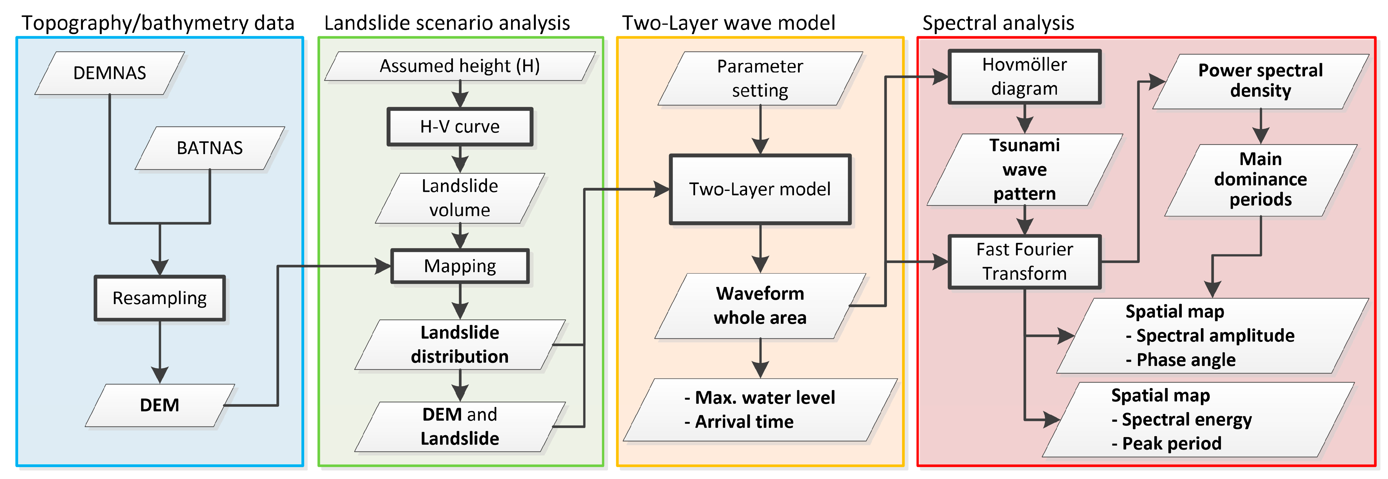
The methodology employed in this study encompasses four key components: topography/bathymetry data, landslide scenario analysis, two-layer wave propagation modeling, and spectral analysis, as shown in the streamline in Figure 11. To establish a comprehensive understanding of the study area’s land and underwater terrain, extensive topography and bathymetry data were collected and utilized. This dataset serves as a crucial foundation for subsequent analyses, enabling accurate modeling and interpretation of tsunami events. A thorough investigation of the landslide scenario was conducted to explore the potential causes and impacts of tsunamis in the region. The focus of this study was to assess the characteristics of the 1674 tsunami in Piru Bay, assuming it was caused by a submarine landslide triggered by seismotectonic movement, as suggested by Pranantyo and Cummins [10]. To simulate the propagation of tsunamis, a two-layer wave propagation model was employed. This model incorporates the characteristics of the coastal environment, including the interaction between the tsunami wave and the seabed. By utilizing this model, predictions of wave behavior and its impact on coastal areas were made. Spectral analysis techniques, specifically the fast Fourier transform (FFT), were applied to the collected data. This analysis allowed for the identification and analysis of different frequencies and amplitudes present in the tsunami signals. It provided valuable insights into dominant wave periods and energy distribution, enhancing the understanding of tsunami behavior and potential impacts. By integrating these four components into the methodology, a comprehensive and rigorous approach was established, facilitating a deeper understanding of tsunami dynamics and enhancing the ability to assess and mitigate tsunami risks in the study area.

4.1. Topography and Bathymetry Data

Badan Informasi Geospatial (BIG), an organization in Indonesia, generously supplied comprehensive bathymetric and topographic data encompassing Piru Bay and the surrounding continental areas. The dataset consists of two separate datasets, one providing bathymetry data for the sea with a resolution of 180 m and the other offering topography data for the land with a resolution of 8 m. The bathymetry data was sourced from the National Bathymetric Data (BATNAS) [12], while the topography data was obtained from the Digital Elevation Model Nasional (DEMNAS) [13] provided by Indonesia. To ensure consistency and compatibility, both datasets underwent resampling to a resolution of 180 m, as illustrated in Figure 1b. This resampling process resulted in a grid comprising 686 columns and 646 rows, effectively covering the entire Piru Bay area.

4.2. Landslide Scenario Analysis

The fundamental premise of this study is that the tsunami that occurred in Piru Bay in 1674 was initially believed to have been caused by a submarine landslide resulting from a significant movement of materials originally situated on the upper slope. This movement led to a submarine landslide on the seafloor and the formation of a submarine deposit. This massive slide was likely triggered by seismotectonic activity. The resulting submarine landslide would have generated a tsunami that affected the coastal area of Piru Bay.

The possible locations of the hypothesized landslides in Piru Bay are depicted in Figure 12, and these landslides can be categorized into three scenarios. The three primary landslides identified in Piru Bay were significant contributors to the investigated tsunami. The location of these landslides was previously mentioned in research [9], recommending their proximity to the shoreline between Hila and Seith. Following the recommended location from the previous study [10], the three landslide scenarios were situated accordingly. The size of each submarine landslide was determined based on the relationship between the volume of the landslide ($V$) and the resulting runup height ($H$), as provided by Murty [14]. The relationship is expressed by the formula $H=aV$, where the value of $a$ ranges from 0.3945 to 2.3994. Scenario A (see Figure 12a) represents the smallest landslide, with an estimated volume of approximately 0.14 km³, corresponding to a runup height of approximately 50 m. Scenario B (see Figure 12b) has a volume of around 0.2 km³, estimated based on a runup height of 75 m. Finally, Scenario C (see Figure 12c) represents the largest landslide with an estimated volume of approximately 1.12 km³, corresponding to a runup height of 100 m.

4.3. Two-Layer Wave Propagation Modeling

The method for simulating tsunamis triggered by landslides involves treating both the landslide and the water as distinct fluids [15,16,17,18]. This approach enables the deformation of the landslide and accurately represents the two-way interaction between the landslide and the surrounding water. Extensive efforts have been dedicated to developing such models. For instance, Jiang and Leblond [19,20] introduced a two-layer model that treated the lower-layer landslide as either a laminar incompressible viscous fluid or a Bingham visco-plastic fluid. This model dynamically coupled the deformable underwater landslide with the resulting tsunami waves. Further advancements to this approach were made by Fine et al. [21] and Skvortsov and Bornhold [22]. Abadie et al. [23] utilized a 3D multi-fluid Navier–Stokes model called THETIS to simulate tsunami waves resulting from a potential collapse of the west flank of the Cumbre Vieja Volcano (CVV) in the Canary Islands, Spain. In this model, the landslide and water were treated as immiscible fluids with different densities, and a volume of fluid (VOF) algorithm was employed to accurately capture the free surface and the interface between the landslide and water. Horrillo et al. [24] employed a similar approach. Assier-Rzadkiewicz et al. [25] modeled underwater landslides as sediment-water mixtures, considering rheology that varied from linear fluid viscosity at low sediment concentrations to Bingham visco-plastic behavior at high concentrations. The model successfully replicated the water waves generated by a laboratory landslide with reasonable accuracy. Heinrich et al. [26] implemented the same approach using a 3D Navier–Stokes solver to investigate water waves generated by a potential debris avalanche in Montserrat, Lesser Antilles. Ma et al. [27] adopted a similar approach in the non-hydrostatic wave model NHWAVE, albeit without incorporating the Bingham visco-plastic behavior at high concentrations.

The assessment of the tsunami model in Piru Bay utilizes a two-layer numerical model that was developed to solve nonlinear shallow-water equations. This model incorporates two interfacing layers and appropriate kinematic and dynamic boundary conditions at the seafloor, interface, and water surface [28,29,30]. The aim is to simulate landslide-generated tsunamis by considering the interactions between tsunami generation and submarine landslides as upper and lower layers.

The mathematical model employed in the landslide-tsunami code consists of a stratified medium with two layers. The first layer represents a homogeneous inviscid fluid with a constant density ${\rho }_1$ (1024 kg/m³), representing seawater. The second layer represents a fluidized granular material with a density ${\rho }_s$ of 2000 kg/m³ and a porosity $\phi$ of 0.35. In this study, the mean density of the fluidized debris remains constant and is determined by ${\rho }_2=\left(1-\phi \right){\rho }_s+\phi {\rho }_1$, as stated in previous research [31]. It is assumed that the two fluids, water and fluidized debris, are immiscible in this study. The governing equations are described as follows:

Continuity equation for the first layer:

$$\frac{\partial Z_1}{\partial t}+\frac{\partial Q_{1x}}{\partial x}+\frac{\partial Q_{1y}}{\partial y}=0$$

Momentum equations for the first layer in the $X$ and $Y$ directions:

$$\begin{gathered} \frac{\partial Q_{1x}}{\partial t}+\frac{\partial }{\partial x}\left(\frac{Q_{1x}^2}{D_1}\right)+\frac{\partial }{\partial y}\left(\frac{Q_{1x}{Q}_{1y}}{D_1}\right)+g{D}_1\frac{\partial Z_1}{\partial x}+g{D}_1\frac{\partial Z_2}{\partial x}-{\tau }_{1x}=0 \\ \frac{\partial Q_{1y}}{\partial t}+\frac{\partial }{\partial x}\left(\frac{Q_{1x}{Q}_{1y}}{D_1}\right)+\frac{\partial }{\partial y}\left(\frac{Q_{1y}^2}{D_1}\right)+g{D}_1\frac{\partial Z_1}{\partial y}+g{D}_1\frac{\partial Z_2}{\partial y}-{\tau }_{1y}=0 \end{gathered}$$

Continuity equation for the second layer:

$$\frac{\partial Z_2}{\partial t}+\frac{\partial Q_{2x}}{\partial x}+\frac{\partial Q_{2y}}{\partial y}=0$$

Momentum equations for the second layer in the $x$ and $y$ directions:

$$\begin{gathered} \frac{\partial Q_{2x}}{\partial t}+\frac{\partial }{\partial x}\left(\frac{Q_{2x}^2}{D_2}\right)+\frac{\partial }{\partial y}\left(\frac{Q_{2x}{Q}_{2y}}{D_2}\right)+g{D}_2\frac{\partial Z_2}{\partial x}+g{D}_2\frac{{\rho }_1}{{\rho }_2}\frac{\partial Z_1}{\partial x}-{\tau }_{2x}=0 \\ \frac{\partial Q_{2y}}{\partial t}+\frac{\partial }{\partial x}\left(\frac{Q_{2x}{Q}_{2y}}{D_2}\right)+\frac{\partial }{\partial y}\left(\frac{Q_{2y}^2}{D_2}\right)+g{D}_2\frac{\mathit{\partial }{Z}_2}{\partial y}+g{D}_2\frac{{\rho }_1}{{\rho }_2}\frac{\partial Z_1}{\partial y}-{\tau }_{2y}=0 \end{gathered}$$

(1)

where index 1 pertains to the upper layer and index 2 represents the second layer. $Z_i(x,y,t)$, $i=1, 2$ denotes the level of the layer at each point ($x,y$) at time t, with the level measured from a given reference level. $Q_i(x,y,t)$, $i=1, 2$ denotes the vertically integrated discharge in the x and y directions. $g$ denotes the gravitational acceleration, and ${\rho }_1$ and ${\rho }_2$ are the densities of the first and second layers, respectively. ${\tau }_i(x,y,t)$ represents the bottom stress in each layer at each point $(x,y)$ and time $t$. In Equation (1), the interaction between the first layer and the second layer is determined by the fifth term in the momentum equation.

Equation (1) is solved using a finite difference scheme implemented in the Open Multi-Processing (OpenMP) platform, enabling faster computation. In this model, the landslide layer is considered to be in equilibrium when it has zero velocity. For the generation of the landslide tsunami, the far-field wave propagation and run-up height are based on the tsunami wave.

Numerical tsunami simulations were conducted by utilizing submarine landslide sources to simulate potential tsunami scenarios and gather numerical results along the coasts of Piru Bay. The study utilized bathymetry and topography data with a resolution of 180 m and a computational domain of 686 × 646. The constant-grid tsunami simulation involved solving approximately one million equations and unknowns at each time step, ranging from 0.00001 to 1 s. Non-reflective boundary conditions were applied at the boundary lines representing the open sea, while no specific boundary conditions were set for wet/dry fronts in coastal areas [32].

4.4. Spectral Analysis

Spectral analysis is employed in this study to investigate oscillation patterns and frequency characteristics, building upon previous research conducted by Catalán et al. [33] and Ren et al. [34]. The analysis utilizes the Fourier transform, specifically the fast Fourier transform (FFT) method. The implementation of the FFT is based on the Numpy library within the Python package, as outlined by Harris et al. [35]. By applying the FFT, the spectral amplitude is determined as a function of frequency or period, which is a commonly used technique for analyzing tsunami signals, as demonstrated by Munger and Cheung [36], Roeber et al. [37], Yamazaki and Cheung [38], Heidarzadeh and Satake [39], Pakoksung et al. [40], and Wang et al. [41].

The wave pattern along the shoreline was analyzed using a Hovmöller diagram to observe wave reflection and edge waves [11]. The Hovmöller diagram is commonly used to illustrate wave behavior, with the axes representing changes over the time series of scalar quantities like wave amplitude. Initially introduced by Ernest Hovmöller [42] for atmospheric waves, we employed the Hovmöller diagram in this study, with the horizontal axis representing distance along the shoreline and the vertical axis representing the time series.

To analyze the simulated waveform of the event, a Fast Fourier Transform (FFT) was applied, considering a time series of 5 h following the eruption based on the wave pattern in the Hovmöller diagram. By plotting the spectra, the spatial distribution of period and amplitude was visualized, enabling the identification of dominant amplitudes within specific periods using the power spectral density. The power spectral density (PSD), or spectral energy, represents the distribution of the average power of a wave in the frequency domain and can be estimated by squaring the FFT [43]. Through spectral analysis of the time series wave, the dominant periods were estimated based on the power spectral density along the coastline of Piru Bay.

By employing spectral analysis, this study aims to gain insights into the oscillation patterns and frequency characteristics of the tsunami wave. The Fourier transform, specifically the fast Fourier transform (FFT), is utilized, drawing from the Numpy library in the Python package, as described by Harris et al. [35]. The analysis focuses on the simulated waveform of the event, spanning a time series of 5 h after the eruption. Spectra are plotted to provide a spatial representation of the relationship between period and spectral amplitude, enabling the identification of dominant periods along the coastline of Piru Bay. The spectra plot also illustrates the spatial relationship between period and phase angle. In the frequency domain, a wave signal is represented by its frequency spectrum. The wave signal spectrum comprises an amplitude spectrum and a phase spectrum. The amplitude spectrum indicates the amplitude of the wave signal components as a function of their frequencies. The phase spectrum indicates the phase of the wave signal components as a function of their frequencies, measured relative to a cosine waveform [44]. The spatial peak period was determined by identifying the maximum amplitude in the amplitude spectrum.

References

- Hamilton, W. Tectonics of the Indonesian Region, 4th ed.; United States Government Printing Office: Washington, DC, USA, 1979.
- McCaffrey, R. Active tectonics of the eastern Sunda and Banda arcs. J. Geophys. Res. Solid Earth 1988, 93, 15163–15182. [Google Scholar] [CrossRef]
- Spakman, W.; Hall, R. Surface deformation and slab-mantle interaction during Banda arc subduction rollback. Nat. Geosci. 2010, 3, 562. [Google Scholar] [CrossRef]
- Pownall, J.; Hall, R.; Lister, G. Rolling open Earth’s deepest forearc basin. Geology 2016, 44, 947–950. [Google Scholar] [CrossRef]
- Rumphius, G.E. Waerachtigh Verhael van de Schuckelijcke Aerdbebinge; Dutch East Indies: Batavia, Indonesia, 1675. [Google Scholar]
- Rumphius, G.E. True History of the Terrible Earthquake. Buijze, W., Ed.; Available online: https://iotic.ioc-unesco.org/1950-ambon-tsunami/1674-tsunami-in-ambon-and-seram/ (accessed on 19 June 2023).
- Løvholt, F.; Kühn, D.; Bungum, H.; Harbitz, C.B.; Glimsdal, S. Historical tsunamis and present tsunami hazard in eastern Indonesia and the southern Philippines. J. Geophys. Res. Solid Earth 2012, 117, B09310. [Google Scholar] [CrossRef]
- Harris, R.; Major, J. Waves of destruction in the East Indies: The Wichmann catalogue of earthquakes and tsunami in the Indonesian region from 1538 to 1877. Geol. Soc. Lond. Spec. Public 2017, 441, 9–46. [Google Scholar] [CrossRef]
- Gusman, A.R.; Satake, K.; Shinohara, M.; Sakai, S.; Tanioka, Y. Fault slip distribution of the 2016 Fukushima earthquake estimated from tsunami waveforms. Pure Appl. Geophys. 2017, 174, 2925–2943. [Google Scholar] [CrossRef]
- Pranantyo, I.R.; Cummins, P.R. The 1674 Ambon Tsunami: Extreme Run-Up Caused by an Earthquake-Triggered Landslide. Pure Appl. Geophys. 2020, 177, 1639–1657. [Google Scholar] [CrossRef]
- Hovmöller, E. The trough-and-Ridge diagram. Tellus 1949, 1, 62–66. [Google Scholar] [CrossRef]
- National Bathymetric Data (BATNAS). Available online: https://tanahair.indonesia.go.id/demnas/#/batnas (accessed on 1 April 2023).
- Digital Elevation Model Nasional (DEMNAS). Available online: https://tanahair.indonesia.go.id/demnas/#/demnas (accessed on 1 April 2023).
- Murty, T.S. Tsunami wave height dependence on landslide volume. Pure Appl. Geophys. 2003, 160, 2147–2153. [Google Scholar] [CrossRef]
- Ren, Z.; Liu, H.; Li, L.; Wang, Y.; Sun, Q. On the effects of rheological behavior on landslide motion and tsunami hazard for the Baiyun Slide in the South China Sea. Landslides 2023, 20, 1599–1616. [Google Scholar] [CrossRef]
- Sun, Q.; Wang, Q.; Shi, F.; Alves, T.; Gao, S.; Xie, X.; Wu, S.; Li, J. Runup of landslide-generated tsunamis controlled by paleogeography and sea-level change. Commun. Earth Environ. 2022, 3, 244. [Google Scholar] [CrossRef]
- Sun, Q.; Alves, T.M.; Lu, X.; Chen, C.; Xie, X. True volumes of slopefailure estimated from a Quaternarymass-transport deposit in the northern South China Sea. Geophys. Res. Lett. 2018, 45, 2642–2651. [Google Scholar] [CrossRef]
- Gao, J.; Ma, X.; Chen, H.; Zang, J.; Dong, G. On hydrodynamic characteristics of transient harbor resonance excited by double solitary waves. Ocean. Eng. 2021, 219, 108345. [Google Scholar] [CrossRef]
- Jiang, L.; Leblond, P.H. The coupling of a submarine slide and the surface waves which it generates. J. Geophys. Res. 1992, 97, 12731–12744. [Google Scholar] [CrossRef]
- Jiang, L.; Leblond, P.H. Numerical modeling of an underwater bingham plastic mudslide and the waves which it generates. J. Geophys. Res. 1992, 98, 10303–10317. [Google Scholar] [CrossRef]
- Fine, I.; Rabinovich, A.; Bornhold, B.; Thomson, R.; Kulikov, E. The grand banks landslide-generated tsunami of November 18, 1929: Preliminary analysis and numerical modeling. Mar. Geol. 2005, 215, 45–57. [Google Scholar] [CrossRef]
- Skvortsov, A.; Bornhold, B. Numerical simulation of the landslide-generated tsunami in Kitimat Arm, British Columbia, Canada, 27 April 1975. Geophys. Res. 2009, 35, 131–136. [Google Scholar] [CrossRef]
- Abadie, S.; Harris, J.C.; Grilli, S.T.; Fabre, R. Numerical modeling of tsunami waves generated by the flank collapse of the Cumbre Vieja volcano (La Palma, Canary islands): Tsunami source and near field effects. J. Geophys. Res. 2012, 117, C05030. [Google Scholar] [CrossRef]
- Horrillo, J.; Wood, A.; Kim, G.-B.; Parambath, A. A simplified 3d Navier–Stokes numerical model for landslide-tsunami: Application to the Gulf of Mexico. J. Geophys. Res. Oceans 2013, 118, 6934–6950. [Google Scholar] [CrossRef]
- Assier-Rzadkiewicz, S.; Mariotti, C.; Heinrich, P. Numerical simulation of submarine landslides and their hydraulic effects. J. Waterw. Port Coast. Ocean Eng. 1997, 123, 149–157. [Google Scholar] [CrossRef]
- Heinrich, P.; Mangeney, A.; Guibourg, S.; Roche, R.; Boudon, G.; Cheminee, J.-L. Simulation of water waves generated by a potential debris avalanche in Montserrat, Lesser Antilles. Geophys. Res. Lett. 1998, 25, 3697–3700. [Google Scholar] [CrossRef]
- Ma, G.; Kirby, J.T.; Shi, F. Numerical simulation of tsunami waves generated by deformable submarine landslides. Ocean Modell. 2013, 69, 146–165. [Google Scholar] [CrossRef]
- Imamura, F.; Imteaz, M.A. Long waves in two-layers: Governing equations and numerical model. Sci. Tsunami Hazards 1995, 13, 3–24. [Google Scholar]
- Pakoksung, K.; Suppasri, A.; Imamura, F.; Athanasius, C.; Omang, A.; Muhari, A. Simulation of the Submarine Landslide Tsunami on 28 September 2018 in Palu Bay, Sulawesi Island, Indonesia, Using a Two-Layer Model. Pure Appl. Geophys. 2019, 176, 3323–3350. [Google Scholar] [CrossRef]
- Pakoksung, K.; Suppasri, A.; Muhari, A.; Syamsidik; Imamura, F. Global optimization of a numerical two-layer model using observed data: A case study of the 2018 Sunda Strait tsunami. Geosci. Lett. 2020, 7, 15. [Google Scholar] [CrossRef]
- Macías, J.; Vázquez, J.T.; Fernández-Salas, L.M.; González-Vida, J.M.; Bárcenas, P.; Castro, M.J.; Díaz-del-Río, V.; Alonso, B. The Al-Borani submarine landslide and associated tsunami. A modelling approach. Mar. Geol. 2015, 361, 79–95. [Google Scholar] [CrossRef]
- Imamura, F. Review of tsunami with a finite difference method. In Long-Wave Runup Models; World Scientific Pub Co., Inc.: Singapore, 1995; pp. 25–42. [Google Scholar]
- Catalán, P.A.; Aránguiz, R.; González, G.; Tomita, T.; Cienfuegos, R.; González, J.; Shrivastava, M.N.; Kumagai, K.; Mokrani, C.; Cortés, P.; et al. The 1 April 2014 Pisagua tsunami: Observations and modeling. Geophys. Res. Lett. 2015, 42, 2918–2925. [Google Scholar] [CrossRef]
- Ren, Z.; Hou, J.; Wang, P.; Wang, Y. Tsunami resonance and standing waves in Hangzhou bay. Phys. Fluids 2021, 33, 81702. [Google Scholar] [CrossRef]
- Harris, C.R.; Millman, K.J.; Van Der Walt, S.J.; Gommers, R.; Virtanen, P.; Cournapeau, D.; Wieser, E.; Taylor, J.; Berg, S.; Smith, N.J.; et al. Array programming with NumPy. Nature 2020, 585, 357–362. [Google Scholar] [CrossRef]
- Munger, S.; Cheung, K.F. Resonance in hawaii waters from the 2006 kuril islands tsunami. Geophys. Res. Lett. 2008, 35, L07605. [Google Scholar] [CrossRef]
- Roeber, V.; Yamazaki, Y.; Cheung, K.F. Resonance and impact of the 2009 Samoa tsunami around Tutuila, American Samoa. Geophys. Res. Lett. 2010, 37, L12605. [Google Scholar] [CrossRef]
- Yamazaki, Y.; Cheung, K. Shelf resonance and impact of near filed tsunami generated by the 2010 Chile earthquake. Geophys. Res. Lett. 2011, 38, L12605. [Google Scholar] [CrossRef]
- Heidarzadeh, M.; Satake, K. Waveform and spectral analyses of the 2011 Japan tsunami records on tide gauge and dart stations across the pacific ocean. Pure Appl. Geophys. 2013, 170, 1275–1293. [Google Scholar] [CrossRef]
- Pakoksung, K.; Suppasri, A.; Imamura, F. The near-field tsunami generated by the 15 January 2022 eruption of the Hunga Tonga-Hunga Ha’apai volcano and its impact on Tongatapu, Tonga. Sci. Rep. 2022, 12, 15187. [Google Scholar] [CrossRef]
- Wang, Y.; Su, H.-Y.; Ren, Z.; Mz, Y. Source properties and resonance characteristics of the tsunami generated by the 2021 M 8.2 Alaska Earthquake. J. Geophys. Res. Ocean. 2022, 127, e2021JC018308. [Google Scholar] [CrossRef]
- Melgar, D.; Ruiz-Angulo, A. Long-lived tsunami edge waves and shelf resonance from the M8.2Tehuantepec earthquake. Geophys. Res. Lett. 2018, 45, 12414–12421. [Google Scholar] [CrossRef]
- Dempster, J. Signal Analysis and Measurement. In Biological Techniques Series, The Laboratory Computer; Academic Press: Cambridge, MA, USA, 2001; pp. 136–171. [Google Scholar] [CrossRef]
- Randall, R.B. Cepstrum Analysis, Encyclopedia of Vibration; Elsevier: Amsterdam, The Netherlands, 2001; pp. 216–227. [Google Scholar] [CrossRef]
Figure 1.
Study area. (
a) The red box in the global map is the location of the Banda Sea. The red line represents the tectonics in the Banda Sea: Seram Megathurst (SMT), Kawa fault (KF), South Seram Thrust (SST), Banda Detachment (BD), Wetar thrust (WT), and Wetar-Atauro fault (WAF). (
b) The detail of bathymetry/topography data located in the yellow box of the
Figure 1a is the area used to simulate the tsunami. Tsunami heights are indicated by the red point at 100 m and the blue point at 5 m.
Figure 2.
Temporal generation of the tsunami wave for demonstrating in Scenario C after (a) 5 s; (b) 15 s; (c) 30 s; (d) 60 s; (e) 90 s, and (f) 120 s.
Figure 3.
Maximum water level, the top panel presented the maximum water level on the north shoreline of the bay, and the bottom panel showed the south. (a) Scenario A, (b) Scenario B, and (c) Scenario C.
Figure 4.
Inundation depth distribution in the inland area. (a) Scenario A; (b) Scenario B; and (c) Scenario C.
Figure 5.
Arrival time of the tsunami, the top panel presented the maximum water level on the north shoreline of the bay, and the bottom panel showed the south. (a) Scenario A, (b) Scenario B, and (c) Scenario C.
Figure 6.
Impact of the tsunami along the coastline that the black dot is represented by the observed height of tsunami runup. (a) The coastline on the northern side; and (b) the coastline on the southern side.
Figure 7.
Hovmöller diagram showing the time generation of the tsunami at virtual tide gauges along the coastline.
Figure 8.
(a) Power spectral density (PSD) at virtual tide gauges along the coast. (b) Average PSD of the virtual tide gauge along the coast.
Figure 9.
Resonance modes in Piru Bay during the dominance period. The first column presents the spectral amplitude; (a1) 6.96 min, (b1) 5.16 min, (c1) 4.1 min, (d1) 3.75 min, (e1) 3.36 min. The second column shows the phase angle; (a2) 6.96 min, (b2) 5.16 min, (c2) 4.1 min, (d2) 3.75 min, (e2) 3.36 min.
Figure 10.
(a) Spectral energy and (b) peak period in Piru Bay.
Figure 11.
Streamline of this study to estimate the tsunami wave characteristics based on landslide scenarios.
Figure 12.
Landslide scenario, the top panel presented the top view of each scenario and the bottom panel showed the profiling of the landslide. (a) Scenario A, (b) Scenario B, and (c) Scenario C.