Article

In Situ Skin Friction Capacity Modeling with Advanced Neuro-Fuzzy Optimized by Metaheuristic Algorithms

by
Mohammed A. Mu’azu
Department of Civil Engineering, University of Hafr Al-Batin, Al Jamiah District 39524, Hafr Al Batin P.O. Box 1803, Saudi Arabia
Geotechnics 2022, 2(4), 1035-1058; https://doi.org/10.3390/geotechnics2040049
Submission received: 3 October 2022 / Revised: 25 November 2022 / Accepted: 25 November 2022 / Published: 1 December 2022

Abstract

:
Developing new optimization algorithms and data mining has improved traditional engineering structural analysis models (meaning basically swarm-based solutions). Additionally, an accurate quantification of in situ friction capacity (ISFC) of driven piles is of paramount importance in design/construction of geotechnical infrastructures. A number of studies have underscored the use of models developed via artificial neural networks (ANNs) in anticipation of the bearing capacity of driven piles. Nonetheless, the main drawbacks of implementing the techniques relying on artificial neural networks are their slow convergence rate and reliable testing outputs. The current research focused on establishing an accurate/reliable predictive network of ISFC. Therefore, an adaptive neuro-fuzzy inference system (ANFIS) coupled with Harris hawk optimization (HHO), salp swarm algorithm (SSA), teaching-learning-based optimization (TLBO), and water-cycle algorithm (WCA) is employed. The findings revealed that the four models could accurately assimilate the correlation of ISFC to the referenced parameters. The values of the root mean square error (RMSE) realized in the prediction phase were 8.2844, 7.4746, 6.6572, and 6.8528 for the HHO-ANFIS, SSA-ANFIS, TLBO-ANFIS, and WCA-ANFIS, respectively. The results depicted WCA-ANFIS as more accurate than the three other algorithms at the testing and training phase, and could probably be utilized as a substitute for laboratory/classical methods.

1. Introduction

The process of discovering the optimum combination of a set of decision variables to solve a certain issue is referred to as an optimization algorithm. The issue of engineering optimization could be considered a constrained optimization problem, and it is one of the most significant challenges in practical problems [1,2,3]. It is challenging to identify the optimal worldwide solution to complicated optimization problems appearing in diverse domains, including engineering, economics, and medicine, employing traditional mathematical optimization approaches. The strategy has the benefit of being quicker to implement due to its decreased complexity. Nevertheless, its drawback is that it could get stuck in the local region, preventing it from obtaining the optimal global solution. Swarm intelligence optimization algorithms that simulate the behavior of actual organisms and have effectively resolved numerous complicated optimization problems [4,5,6] are also categorized into two main types: evolutionary algorithms and swarm intelligence algorithms [7]. Evolutionary algorithms rely on a biological evolution-inspired system that comprises four operators: random selection, reproduction, recombination, and mutation. The swarm intelligence algorithm is a population-based algorithm that has emerged through social behavior. Meta-heuristic optimization algorithms evolve rapidly [8,9] due to their simple idea, adaptability, and capability to prevent local optima, and are frequently employed to solve various complicated real-world optimization problems [10]. Meta-heuristics could be separated into three primary types depending on the algorithmic inspiration: techniques based on evolution, physics, and swarm intelligence. The laws of natural evolution serve as the basis for evolutionary algorithms [11].
The ANFIS is amongst the most frequently used training systems, and the general usage in geotechnical engineering is well explained in Cabalar et al. [12]. Regarding this study’s aim, it is worth noting that ANFIS was improved using several optimization techniques to envision the applicability of the approaches used in this investigation [13,14]. Numerous research [15,16,17] has shown the effective application of ANFIS in many engineering disciplines. Generally, two constructive variables of the ANFIS method contain steady and mean input and output membership functions [18]. The gradient-based techniques are commonly applied to regulate these parameters. One of the main problems in the gradient-based methods is that the answer is trapped within the local optimality, leading to a slow convergence rate [19,20]. Optimization algorithms can be used as a helpful solution, for example ALO [21], GOA [22], modeling, and uncertainty analysis of groundwater levels using optimized ANFIS with six different optimization algorithms. A best-fit combination of ANFIS-GOA was a superior model (having R2 equal to 0.94). Sun et al. [23] presented an innovative model for predicting the pile bearing capacity. It is modeled as a hybrid firefly algorithm (FA) with ANFIS, achieving a high certainty and more significant than conventional ANFIS. Yu [24] applied ALO-ANFIS and GOA-ANFIS models to estimate the pile settlement located in the Klang Valley project constructed in Kuala Lumpur, Malaysia. They have found that the ALO-ANFIS (having the R2 of 0.9077 for training data and 0.9387 for testing) shows superior performance compared to GOA-ANFIS. Shirazi et al. [25] developed a mineralogical map by utilizing a proposed Neuro-Fuzzy-Analytic Hierarchy Process (NF-AHP) technique, verified with documented minerals deposits, showing that NF-AHP has a possible potential application in another metallogenic province. Moayedi and Hayati [26] presented ANFIS as a capable method for forecasting the ISFC. In their study, ANFIS showed a surpass convergence behavior compared to genetic programming (GP) and support vector machine (SVM) [27,28,29]. Prayogo and Susanto [30] estimated the FC of driven piles by applying a metaheuristic algorithm with a least-squares SVM. Gray wolf optimization (GWO) was coupled with ANFIS and multilayer perceptron (MLP) separately to predict the UBC of the piles. The findings revealed that both the MLP and ANFIS approaches could predict the piles’ UBC; however, the MLP-GWO model performed significantly [31]. Armaghani et al. [32] obtained more precise expected values of pile bearing capacity when the competitive imperialism algorithm (ICA) is optimized with a system of ANFIS-group method of data handling (GMDH) to form a hybridized ANFIS-GMDH-ICA, in comparison to those achieved by ANFIS-GMDH predictive models. ANFIS-GMDH-ICA may be a sophisticated, practical, and potent approach for foundation engineering and design challenges. Kumar et al. [33] compared the adaptability and applicability of several recently developed systems, namely Minimax Probability Machine Regression (also known as MPMR), Group Method of Data Handling (GMDH), Emotional Neural Network (ENN), and Adaptive Neuro-Fuzzy Inference System (ANFIS) in the assessment of piles embedded in non-cohesive soils. Their findings revealed that the ANFIS (with RMSE of 0.4 for the training dataset and 2.13 for the testing dataset) method outperformed alternative models for the reliability evaluation of pile bearing capacity [34]. In contrast, the ENN (RMSE of 2.03 in training and 31.24 in testing) model performed as the least accurate model. Liang et al. [35] employed three hybrid artificial neural networks (ANNs) to predict the FC affected by four factors mentioned in Goh [36]. The RMSE and the R2 achieved in the prediction phase show that the black hole algorithm (BHA) is more promising than the firefly algorithm (FA) and multi-tracker optimization algorithm (MTOA); however, MTOA has the highest precision in training. Haidari et al. [37] first introduced HHO for simulating hunting Harris’ hawks. Since then, it has been used to analyze various optimization problems with greater benefits than other swarm-based OAs because it does not require any parameters or derivative equations. It only requires the initial population of the swarm. The most beneficial aspect of HHO is its harmony between exploration and exploitation. It is solid, complete, and simple to utilize. As the number of HHO iterations rises, so does the capacity for exploration, and it has a proven outstanding performance in several real-time optimizations compared to other metaheuristic algorithms [38]. Because of such advantages, HHO and its variants have lately been commonly employed for real-world challenges. HHO has greatly succeeded in various domains and applications [39,40,41,42]. Wang et al. [43] suggested an enhanced hybrid Aquila Optimizer (AO) and HHO that outperforms the basic AO and HHO in terms of global search performance and convergence speed compared to standard and CEC2017 benchmark functions. Alabool et al. [44] carried out a comprehensive review on HHO and its variant, and postulated that it is easy to execute, well structured, and flexible. Nevertheless, since there is no one ideal optimizer for all potential computing tasks, population diversity, convergence rate, and the balance between exploration and exploitation of HHO must all be improved in multi-objective, complicated, and composite optimization situations [45]. Chantar et al. [46] suggested another hybrid optimizer solution called “Binary Harris Hawks Optimizer,” hybridized with the time-varying scheme (briefly called BHHO-TVS) for the classification process [47]. The proposed technique achieves the greatest accuracy rates on 67 percent of datasets compared to similar feature selection algorithms published in previous studies. In addition, the HHO could be used to resolve problems involving unidentified kinds of search space and discrete and continuous spaces [48,49], to improve solution quality [50,51,52], extract optimum parameters with high precision [53,54], and improve prediction performance [55,56]. In 2017, Mirjalili et al. [57] developed a novel swarm intelligence optimization algorithm whose optimization approach was inspired by the salp swarm chain foraging in the ocean (also called the SSA). Due to its simple design and basic implementation, the essential SSA random search optimization technique attracted several researchers’ attention. SSA’s searching behavior as a meta-heuristic algorithm is separated into two major phases: exploration and exploitation. During the exploration phase, it can effectively find the search space mostly by randomization, although it may encounter unexpected modifications. In the period of exploitation, it converges on the most promising location. SSA may therefore be used to solve a variety of research difficulties. SSA seems to be an innovative and promising technique previously applied successfully in several situations. It has a distinct benefit in simply having one parameter (r1) for balancing exploration and exploitation. Abualigah et al. [58] carried out a critical review of SSA. They hypothesized that SSA is highly feasible for continuing community employment while highlighting its weaknesses, limitations, and drawbacks. Invoking the no free lunch (NFL) theorem, no optimization algorithm can solve all optimization problems. Because of the limited set F of benchmark functions that must equalize with the objective function in F, SSA may require adjustment and alteration when solving certain real-world optimization issues. Second, SSA has a single objective function, which allows it to handle only single-objective optimization problems. Specific operators must solve binary, discrete, continuous, dynamic, multi-objective, and other issues [59]. The major disadvantage of SSA is its limited capacity to regulate the challenges of multimodal search methods since all three parameters (a, v, and F) appear to converge to the identical solution. Due to its stochastic character and shortage of balance between exploration and exploitation, SSA suffers from the issue of delayed convergence and is frequently trapped in local optima.
Rao et al. [60] popularized the TLBO algorithm, lacking any set of rules and specification data, and applied mechanical design optimization problems to show superiority over other population-based optimization in terms of the best solution, average solution, convergence rate, and computational effort with the potential to be easily extended to other engineering design optimization problems like prediction ISFC. It employs the impact of a teacher’s influence on students, separated into the “Teacher Phase” and “Learner Phase.” It needs only simple governing parameters like the magnitude of population and number of generations to function. TLBO is a nature-inspired population-based algorithm utilizing a population of solutions to proceed to the global solution and is widely accepted by optimization researchers. TLBO, which appears to follow a similar traditional approach to the instructor’s teaching method and the studying or exam process of the students, depending on the physical phenomena of learning, is an essential heuristic algorithm for optimization applications [61,62,63]. The population size with iteration number is the most essential condition of the TLBO. It consistently ignores parameters in its work and has a quick convergence velocity and good searching accuracy. Since the TLBO commenced its work, it has successfully resolved various difficulties because it has attracted the interest of scientists [64] in several fields. Chen et al. [65] combined TLBO with learning enthusiasm-based (LebTLBO) to analyze three excellent control issues in chemical engineering. The results depict its potential capability to achieve the intended purpose. Zhao et al. [66] hybridized MLP with shuffled complex evolution (SCE) as SCE-MLP and TLBO-MLP ensembles to predict CSC; prediction errors were lowered. In addition, SCE is a considerably more time-efficient optimizer concerning computation time.
Eskandar et al. [67] suggested the water cycle algorithm. The inspiration for WCA originated from viewing nature and researching the water cycle and analyzing how streams and rivers flow downhill toward the sea in the natural world. A river or stream is formed when water flows from a higher point to a lower one. As a result, most rivers originate at the summits of mountains, where snow melts. In turn, the rivers continually flow down, replenishing water from rainfall and other streams along the way until ending up in the sea. Even though the innovative water cycle algorithm may solve the issue of entrapment at local optima, its efficiency as a spam classifier is still questionable. Unlike other optimization algorithms, including the Harmony Search algorithm, the WCA has just three control parameters. Employing an evaporation strategy, WCA as a feature selector may handle the problem of quick convergence of local optima entrapment [68]. The analysis and development of innovative ways for dealing with FS and cruse dimensionality difficulties are still active research areas, notably for spam classifiers. As a result, the FS methods are being evaluated for the purposes mentioned above: (a) improved performance (perhaps prediction accuracy or learning speed); (b) data simplification for model selection; and (c) removal of redundant or unnecessary features (dimensionality reduction) [69]. Noting that, feature selection or reduction strategies have been used in several types of research during the last ten years. Such a strategy has proven practical outputs for many published examples.
Furthermore, this study has concentrated on enhancing the effectiveness of the method. This section covers a variety of relevant technologies and methodologies depending on metaheuristic techniques [70], such as local search and population-based methods for both hybrid and heuristics metaheuristics [71,72,73,74,75]. Moayedi and Mosavi [76] employed WCA-MLP to test a finite dataset to estimate the settlement, and the outcomes are correlated with electromagnetic field optimization (EFO) and SCE benchmarks [77]. It was discovered that the training error of WCA is less than that of EFO and SCE, while the accuracy of WCA-MLP is more prominent in the testing phase rather than the learning phase [76]. The WCA is a powerful investigation approach widely utilized in various applications, as demonstrated in Foong et al. [78] and Nasir et al. [79]. WCA gained popularity because of its capacity to offer an optimum solution while swiftly converging [80]. WCA was effectively used for diverse engineering in a short period [81,82,83]. The advantage of WCA over other explored approaches is demonstrated in [84,85], which is why the algorithm continues to attract increasing attention from academics. WCA has been used lately to predict the bearing capacity of shallow foundations [76]. Multiple successful applications of HHO, SSA, TLBO, and WCA inspired the researcher to modify and use hybridized versions of the above algorithms for the first time to solve the problematic issue of ISFC prediction [86,87,88,89]. However, the uncertainty from theoretical, experimental, and numerical methods of friction capacity estimation for piles under axial compressive loading resulting from complexity of soil-pile interaction, prompted utilization of metaheuristic approach to reliably and accurately predict an in situ friction capacity of piles. Goh [36] stated that the length and diameter of the pile, shear strength, and vertical stress are four factors affecting ISFC prediction. These factors are incorporated to predict the ISFC of the pile with an ANFIS hybridized with HHO, SSA, TLBO, and WCA.
The remaining sections of the paper are structured as follows. Using the information from the prior research, Section 2 provides definitions for the various significant terms. The strategies and procedures that we have developed for our work with deep neural networks are detailed in Section 3. The exploratory configuration employed to execute the recommended strategy and the findings produced for categorizing default customers are described in Section 4. Conclusions and prospective research plans are covered in Section 5.

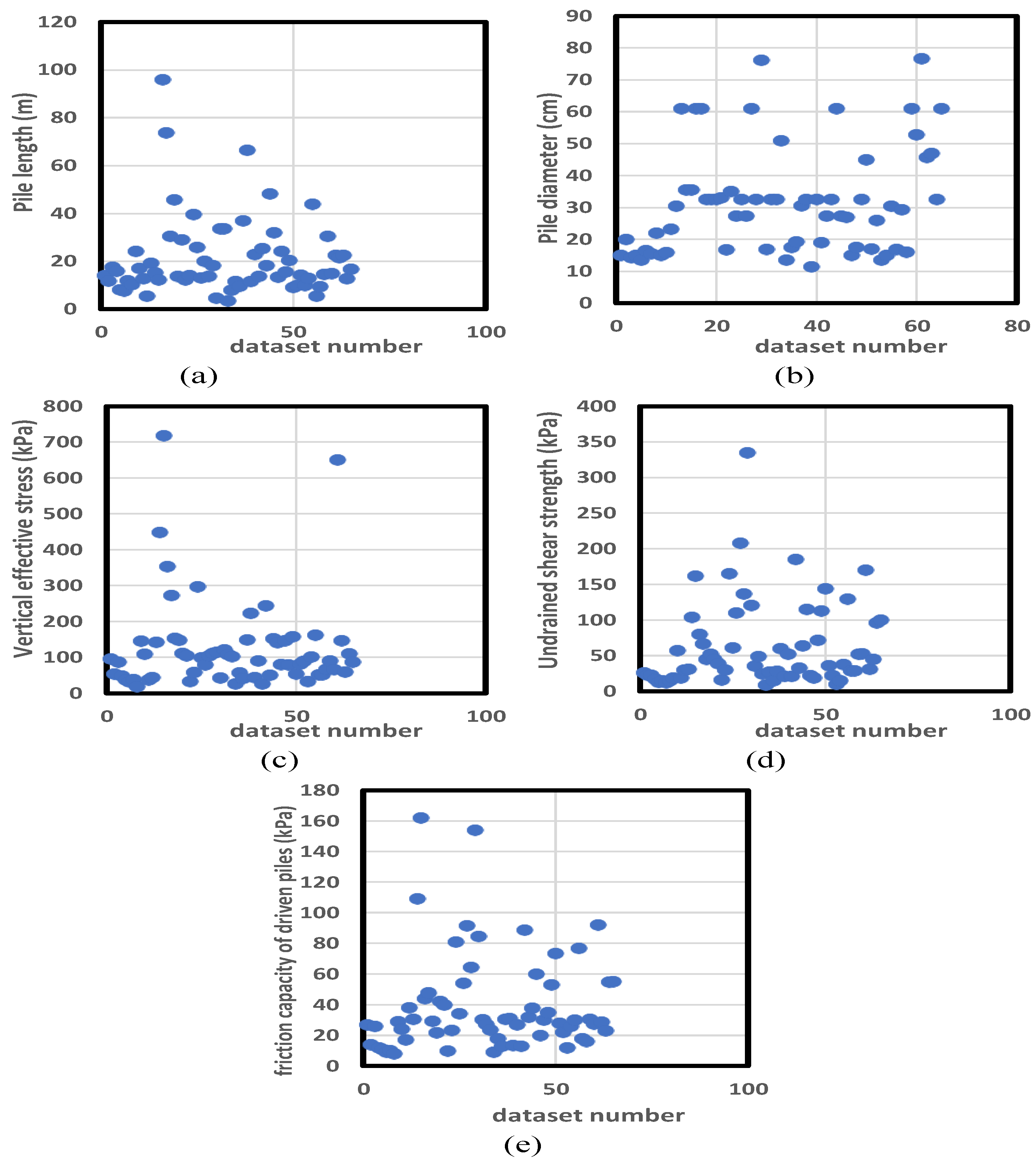
2. Established Database

Sixty-five in situ tests were conducted to generate the datasets. The data from Goh [90] were used to develop the optimal structure (e.g., GOA, WDO, SHO, and MFO) using MLP models. Additionally, the results of pile load tests are collected, as are data on the nearby soil properties. As a result, the training and testing sets are built on the basis of extensive in situ investigations. Both models are trained on a dataset of 52 field experiments, and then tested on a dataset of 11 tests. Both the input data (for example, the pile length (m) and diameter (cm)) and the output data (for example, the friction capacity of installed shafts) and output data layers are shown graphically in Figure 1.

3. Methodology

3.1. Adaptive Neuro-Fuzzy Inference Hybrid (ANFIS)

To develop a set of fuzzy ‘if-then’ rules with a proper membership function for generating the specified input-output pairs, Jang [91] presented ANFIS. This system can classify approximation highly nonlinear functions, identify discrete control systems online, and predict chaotic time series [92]. The input-output data optimize the membership functions (MFs). ANFIS involves tuning a FIS system using a backpropagation algorithm depending on input collected data. A FIS’s basic structure includes three conceptual elements: a rule base that consists of a set of fuzzy rules; a database that describes the membership functions (MFs) utilized in the fuzzy rules; and a reasoning mechanism that performs the inference procedure on the rules and the provided facts to produce a reasonable output or conclusion. Such intelligent systems integrate information, techniques, and procedures from numerous sources. They have human-like skills in a particular domain–they adapt and can perform efficiently in changing environments. In ANFIS, neural networks identify patterns and aid in environmental adaptation. FIS integrates human expertise and executes interface and decision-making [93]. Besides, ANFIS is adjusted via a backpropagation approach utilizing input-output data. Investigators utilized fuzzy theory extensively to illustrate complicated processes by applying ideas and if-then rules. Researchers utilized the fuzzy theory due to its ability to solve complex procedures using the if-then rules approach. The theory of decision-making inspirited it in human life [42,94]. As a result, the artificial neural network (ANN) [92] has been applied to optimize the fuzzy theory as ANFIS to acquire self-learning capabilities [95]. Jang [91] proposes ANFIS as an amalgamation of ANN with a fuzzy method. It has been hypothesized that the ANFIS is preferable to the FIS for analyzing nonlinear issues [96]. According to the ANFIS, a FIS is used in a multilayer feed-forward network for training [97]. FIS membership function (MF) parameters may be learned using the ANFIS’s training of the input data by combining least-squares approaches with backpropagation gradient descent. According to Termeh et al. [98], the ANFIS structure consists of five different layers where neurons in each layer contain adaptive nodes expressed by Equations (1) and (2):
L 1 , i = μ A i ( x )
L 1 , i = μ B i ( y )
The input neurons are defined as x and y. A and B signify linguistic variables, whereas μ A i ( x ) and μ B i ( y ) represent the proposed node’s MFs.
In the 2nd layer, Equation (3) represents the output of each node, which is the result of all input signals to the suggested node:
L 2 , j = W i = μ A i ( x ) μ B i ( y ) , i = 1.2
where W i represents the output of each node.
The layer three nodes consist of the normalized outputs of layer two, while for layer four, a node function is utilized to link every node, as shown in Equations (4) and (5):
L 3 , i = w ¯ l = w i w 1 + w 2 , i = 1.2
L 4 , i = w ¯ l f i = w ¯ i ( p i x + q i y + r i )
where w ¯ l indicates the firepower normalized by layer three p i , q i , and r i specified for the node parameters.
In layer four, the parameters are considered to be result parameters. The total of all input signals is regarded as a single signal to the output. Layer 5 considers the total of all input signals to the output as a single node:
L 5 , 1 = w ¯ l f i = w i f i w i i = 1.2

3.2. Hybrid Optimization Techniques

3.2.1. Harris Hawk Optimization (HHO)

HHO method is firstly proposed by Heidari et al. [37] to solve numerous optimization problems through adopting great teamwork. The algorithm addresses numerous optimization issues by simulating the cooperative behavior of Harris’s hawks. Hawks catch their prey by tracing, encircling, approaching, and eventually attacking. Exploration and exploitation are the two major stages of the HHO. Waiting, searching, and identifying the prospective prey are part of the initial phase. Let P r a b i t represent the rabbit position, while the hawks’ position is described in the following:
P ( i t e r + 1 ) = { P r a n d ( i t e r ) r 1 | P r a n d ( i t e r ) 2 r 2 P ( i t e r ) |                                   i f   q 0.5 ( P r a b i t ( i t e r ) P m ( i t e r ) ) r 3 ( L B + r 4 ( U B L B ) )       i f   q < 0.5 }
P r a n d is indeed one of the available hawks that are randomly suggested. In addition, r i   (i = 1, 2, 3, 4, q) is a random integer in the range [0,1]. Moreover, P m represents the average position. Considering P i and N as the location of the hawks and their size, respectively, the following equation is used to determine P m .
P m ( i t e r ) = 1 N i = 1 N P i ( i t e r )
In the second stage, let T and E 0 ∈ (−1.1) be the maximum size of the repetitions, and the initial energy, the escaping energy of the hunt (E) that could alter exploration and exploitation, is expressed as follows:
E = 2 E 0 ( 1 i t e r T )
Depending on the magnitude of |E|, it is determined to begin the exploration phase (|E| ≥ 1) or to exploit the solutions’ neighborhood (|E|< 1). In the final phase, depending on the value of |E|, the hawks determine whether to apply a soft (|E|≥ 0.5) or hard (|E|< 0.5) besiege to capture the target from multiple directions. Interestingly, the parameter r is used to compute the target’s escaping probability, if it is more significant than 0.5, the hunt effectively escapes, and if it is less than 0.5, it fails [37].

3.2.2. Salp Swarm Inspired Algorithm (SSA)

Salp swarm-inspired algorithm (SSA) is a new swarm intelligence algorithm evolved in 2017 by Mirjalili et al. [57]. SSA is a population-based strategy that simulates salp swarms’ behavior and social interaction. Salp is a clear marine invertebrate residing in cold water and foraging on plankton. In simulating the salp foraging chain, the salp swarm must be separated into leaders and followers with two distinct update functions. The definitive process of SSA consists of three sections: initialization, the leader’s determination, and updating. The definitive process of SSA consists of three sections: (i) initialization, (ii) determination of the leader, and finally, (iii) updating. The initialization of the objective function is defined by Equation (10):
F = f ( x 1 , x 2 , x 3 x N )
where N is the objective function’s dimension. Assume that the following variables have constant boundaries:
l b i x i u b i                                   ( i = 1 , 2 , 3 , 4 . N )
l b i represents the lower boundary of the i-th variable, whereas u b i represents the upper boundary. Assume the salp swarm’s population is D, commonly known as the number of search agents. Every searching agent’s initial position is specified as:
X D x N = r a n d ( D , N ) × ( U b L b ) + L b
where rand (D, N) is a D × N dimension matrix, of which every element is set to be a random number Rand (D, N) is a D x N matrix. Noting that every member is set by a random number between 0 and 1.
Following the initialization of the salp position, each individual’s position is inserted into the objective function (1), obtaining D fitness values. After that, the D fitness values are sorted, the least fitness value is identified, and the corresponding person is recognized as the leader’s determination. In contrast, the other people are rated as followers from small to large. It is significant to mention that the leader is nearest to the food position (optimal position). As a result, the rows of matrix X are rearranged according to the sorted fitness values. The N-dimensional row vector X1 represents the leader among all D individuals in such a scenario. The i-th component of the leader is signified by X i 1 , where i = 1, 2,3,….., N.. Similarly, the i-th dimension of the j-th follower is denoted by j X i j , where j = 2, 3… D.
The positions of the leader and followers are updated in turn, regarded as updating. The leader position is updated as Equation (13):
X i 1 = { F i + c 1 ( u b i b ) c 2 + l b                     c 3 0.5 F i c 1 ( u b i b ) c 2 + l b                     c 3 < 0.5 }
where Xi is the turned to i-th variable of the leader position, Fi is the individual with the best fitness value in the preceding frame, ub, and lb are the upper and lower bounds of the corresponding dimensional variables, c 1 , c 2 , c 3 are known as three control parameters, and c 2 , c3 are both random numbers between 0 and 1. It seems essential to mention that the leader’s position update is solely connected to the individual position with the optimum fitness value. It has nothing to do with the former positions of other individuals or the leader’s status. The updating direction is set by c 3 , which may be adjusted or omitted from the initial basis. The significant parameter that defines the update step is c 1 . It is described as follows:
c 1 = 2 e ( 4 l L ) 2
where l and L are the current and maximum iterations and e is the natural constant. The lower the number of repetitions, the higher the value of c 1 . The great update step may accelerate the leader’s approach to the optimum global region during the first few iterations. As the number of iterations reaches the maximum number of iterations, the value gradually approaches zero. The locations of the followers are then updated. The followers are attached throughout the foraging process, forming a chain-like combination shape. The chain formation highly influences individuals before and after the followers’ aggressive moves. The position update is dependent on itself and the person in front of it. The formula for updating is as follows:
X j i = 1 2 ( X j i + X i j i )
where X j i denotes the j-th individual’s i-th variable, and X i j i indicates the j-th position of the adjacent individual in front of the j-th individual. All individuals’ fitness values are computed after the leader and follower positions are updated independently. Allowing the followers to reach the leader, the leader’s information is updated once again. A series of iterations complete the optimization.

3.2.3. Teaching-Learning-Based Optimization (TLBO)

TLBO consists of the “Teacher phase” and the “Learner phase.” Rao [60] explains the operation of both phases. During the first phase of the algorithm, the learner receives instruction from the teacher. In contrast, the second part focuses on the learner’s knowledge growth via interaction with peers and acquiring novel information from more experienced learners. At any iteration, i, suppose that there are ‘m’ number of subjects (i.e., design variables), ‘n’ number of learners (i.e., population size, k = 1,2,…,n), and M j , i be the mean result of the learners in a specific subject ‘j’ (j = 1,2,…, m). The greatest learner, kbest, is the individual with the best overall score, Xtotal-kbest, when all topics are evaluated together, and the entire learner population is analyzed. Nevertheless, as the teacher is frequently observed as a competent person who instructs learners to achieve higher results, the algorithm determines the best learner to be the teacher. The difference between the current mean result for every topic and the teacher’s outcome for every subject is represented by Equation (16):
D i f f e r e n c e M e a n j , k , i = r i ( X j , k b e s t , i T F M j , i )
where X j , k b e s t , i is the result of the best learner in subject j. T F is the teaching factor that determines the new value of the mean, whereas r i is a random integer in the range [0,1]. T F may have a value of 1 or 2. T F s value is determined at random with the same probability as,
T F = r a n d [ 1 + r a n d ( 0 , 1 ) { 2 1 } ]
where T F is not a TLBO algorithm parameter. The value of T F is not presented as an input to the method; instead, the algorithm utilizing Equation (17) determines it randomly. Following a series of studies on a variety of benchmark functions, it was determined that the algorithm performs better when the value of T F is between 1 and 2. Nevertheless, the technique performs considerably superior if T F is either 1 or 2; therefore, to simplify the algorithm, the teaching factor is recommended to be either 1 or 2 based on the rounding up requirements stated in Equation (17). According to the d i f f e r e n c e _ M e a n j , k , i , the existing solution is updated in the teacher phase based on the following expression.
X j , k , i = X j , k , i + d i f f e r e n c e _ M e a n j , k , i
where X j , k , i is the updated value of X j , k , i . X j , k , i is accepted if it offers a higher function value. All acceptable function values from the teacher phase are preserved, and such values are used as input in the learner phase. The teacher phase determines the learner phase. The instructor phase influences the learner phase.
On the other hand, the learner phase is the second phase of the algorithm, in which learners improve their knowledge by interacting with one another. A learner communicates with other learners at random to enhance their learning. A learner acquires new information if another learner has greater knowledge. Considering a population size of ‘n,’ randomly select two learners, P, and Q, such that X t o t a l P , i X t o t a l Q , i (where, X t o t a l P , i , i and X t o t a l Q , i , I are the updated function values of Xtotal-P, i and Xtotal-Q, i of P and Q, respectively, at the end of teacher phase).
X j , P , i = X j , P , i + r i ( X j , P , i X j , Q , i )                   i f   X t o t a l P , i < X t o t a l Q , i
X j , P , i = X j , P , i + r i ( X j , Q , i X j , P , i )                   i f   X t o t a l Q , i < X t o t a l P , i
X j , P , i is accepted if it offers a higher function value. Equations (19) and (20) can deal with the minimization issues. Equations (21) and (22) are employed in maximizing problems.
X j , P , i = X j , P , i + r i ( X j , P , i X j , Q , i )                   i f   X t o t a l Q , i < X t o t a l P , i
X j , P , i = X j , P , i + r i ( X j , Q , i X j , P , i )                   i f   X t o t a l P , i < X t o t a l Q , i
More detail could be found in the literature about TLBO in Yan-Kwang et al. [99], Harmandeep et al. [100], and Chen et al. [65].

3.2.4. Water-Cycle Algorithm (WCA)

The water-cycle algorithm (WCA) was designed by Eskandar et al. [67], replicating the water cycle process as an inspiration, imitating how rivers and streams end up in the sea. The steps necessary to execute the WCA could be described as follows:
Step 1: Setting the initial parameters of the WCA algorithm, for instance, 𝐾𝑠𝑟, 𝐾𝑝𝑜𝑝, 𝑑𝑚𝑎𝑥, 𝐼𝑡𝑚𝑎𝑥.
Step 2: Scattering the initial population and determining sea, streams, and rivers.
Assuming 𝐾𝑝𝑜𝑝 as the total size of the population, 𝐾𝑠𝑟 = 1 + the number of rivers, and 𝐾𝑠𝑡𝑟𝑒𝑎𝑚𝑠 (= 𝐾𝑝𝑜𝑝 − 𝐾𝑠𝑟) as the number of streams, Equation (23) illustrates the procedure:
T o t a l   p o p u l a t i o n   = [   S e a     R i v e r   1   S t r e a m   K s r + 1   S t r e a m   K p o p ] = [ x 1 1 x 2 1 x K 1 x 1 2 x 2 2 x K 2 x 1 K p o p x 2 K p o p x K K p o p ]
where river, stream, and sea are each represented by a 1 K-dimensional array as [𝑥1, 𝑥2, …, 𝑥𝐾].
Step 3: The cost of each current population member is calculated by using the following:
C j = C o s t j = f ( x 1 j , x 1 j , , x K j )               j = 1 , 2 , , K p o p
Step 4: Equations (3) and (4) yield the flow intensity of the sea and rivers given N S k as the number of streams emptying into the respective rivers or the sea:
C k = C o s t k C F K s r + 1                   k = 1 , 2 , K s r
N S k = r o u n d { | C k k = 1 K s r C k | x K s t r e a m s }                 k = 1 , 2 , , K s r
Step 5: The following relationships depict the streams and rivers that flow into the sea:
X s t r e a m ( t + 1 ) = X s t r e a m ( t ) + r a n d ( 0 , 1 ) × G × ( X s e a ( t ) X s t r e a m ( t ) )
X s t r e a m ( t + 1 ) = X s t r e a m ( t ) + r a n d ( 0 , 1 ) × G × ( X r i v e r ( t ) X s t r e a m ( t ) )
where G is a variable number between 1 and 2 (close to 2), significantly, once C > 1, streams are permitted to enter rivers from diverse directions.
Step 6: The flow of rivers toward the sea (or downwards) may be expressed as follows:
X r i v e r ( t + 1 ) = X r i v e r ( t ) + r a n d × G × ( X s e a ( t ) X s t r e a m ( t ) )
Step 7: The river is replaced with a stream that provides a better-fitting solution.
Step 8: Likewise, the location of a river that provides a more suitable solution substitutes that of the sea.
Step 9: Using d m a x as a minimal value for managing the intensification level and BU and BL as upper and lower bounds, the preceding algorithm validates the evaporation conditions (for unconstrained issues):
i f | X s e a X r i v e r j | < d m a x         o r       r a n d < 0.1               j = 1 , 2 , , K s r 1
Rain based on Equation (31)
End if
X s t r e a m n e w ( t + 1 ) = B L + r a n d   x   ( B U B L )
Regarding local challenges, the WCA employs the following code to enhance its capacity:
i f | X s e a X s t r e a m j | < d m a x                     j = 1 , 2 , , K N S k
Rain based on Equation (33)
End if
X s t r e a m n e w ( t + 1 ) = X s e a + δ   x   r a n d n ( 1 , K )
r a n d n is a random integer, and δ denotes the variance term indicating the search area around the sea. Equation (32) is only used to avoid early convergence in these issues for streams with natural movements toward the sea. Step 10: The d m a x is reduced as follows:
d m a x ( t + 1 ) = d m a x ( t ) d m a x ( t ) I t m a x
Step 11: The algorithm is finished if any stopping criterion is met.
Step 12: If any stopping criteria are fulfilled, the algorithm is completed; otherwise, the procedure repeats in step 5.
The research uses ANFIS models combined with HHO, SSA, TLBO, and WCA optimization techniques to estimate ISFC. The description of the ANFIS, HHO, SSA, TLBO, and WCA is explained later, while Figure 2 portrays the procedure used in ISFC prediction.

3.3. Data Provision

In order to test the findings, the best-fit predictive network (to predict the ISFC), a proper dataset of driven shafts is prepared. The proposed solutions were mainly affected by four introduced conditional factors, as mentioned in Goh [90]. In this sense, there was a total of 65 samples (e.g., the dataset was collected mainly by Goh [90]), with 52 samples taken for the training (80%) and 13 for testing (20%). The ISFC values are affected by four factors mentioned in Goh [90], playing a vital role as input parameters for the ISFC prediction. Table 1 describes the numerical estimate of the dataset. From Figure 1a–d, the majority of pile length was between 3–33 m, pile diameter was between 10–40 cm, effective vertical stress is between 20–130 kPa, and undrained shear strength was between 10–62 kPa. The ISFC values differ from 9–161 kPa, although 42 records between 9 and 37 kPa.

4. Results and Discussion

Optimization aims to discover all potential outcomes in a search space and determine the optimum solution based on conditions and parameters. Optimization was previously used in engineering and scientific fields, which are inherently complicated to optimize. This motivates the development of various meta-heuristic algorithms to discover the optimal solution. The significance of accurately calculating the friction capacity of driven piles embedded in cohesive soils and its complication in engineering projects is well recognized. This section discusses the HHO-ANFIS, SSA-ANFIS, TLBO-ANFIS, and WCA-ANFIS. The performance and accuracy of the estimated output for the proposed models (e.g., in predicting ISFC) are appraised by measuring MAE, RMSE, and R2, calculated using Equations (35)–(37), respectively.
M A E = 1 G i = 1 G | I S F C i e x p e c t e d I S F C i s i m u l a t e d |
R M S E = 1 G i = 1 G [ I S F C i e x p e c t e d I S F C i s i m u l a t e d ] 2
  R 2 = 1 i = 1 G ( I S F C i s i m u l a t e d I S F C i e x p e c t e d ) 2 i = 1 G ( I S F C i e x p e c t e d I S F C ¯ i e x p e c t e d )
where ISFCi is expected to indicate the expected ISFCs, ISFCi simulated stance for the simulated ones, and G presents the sum of ISFCs.

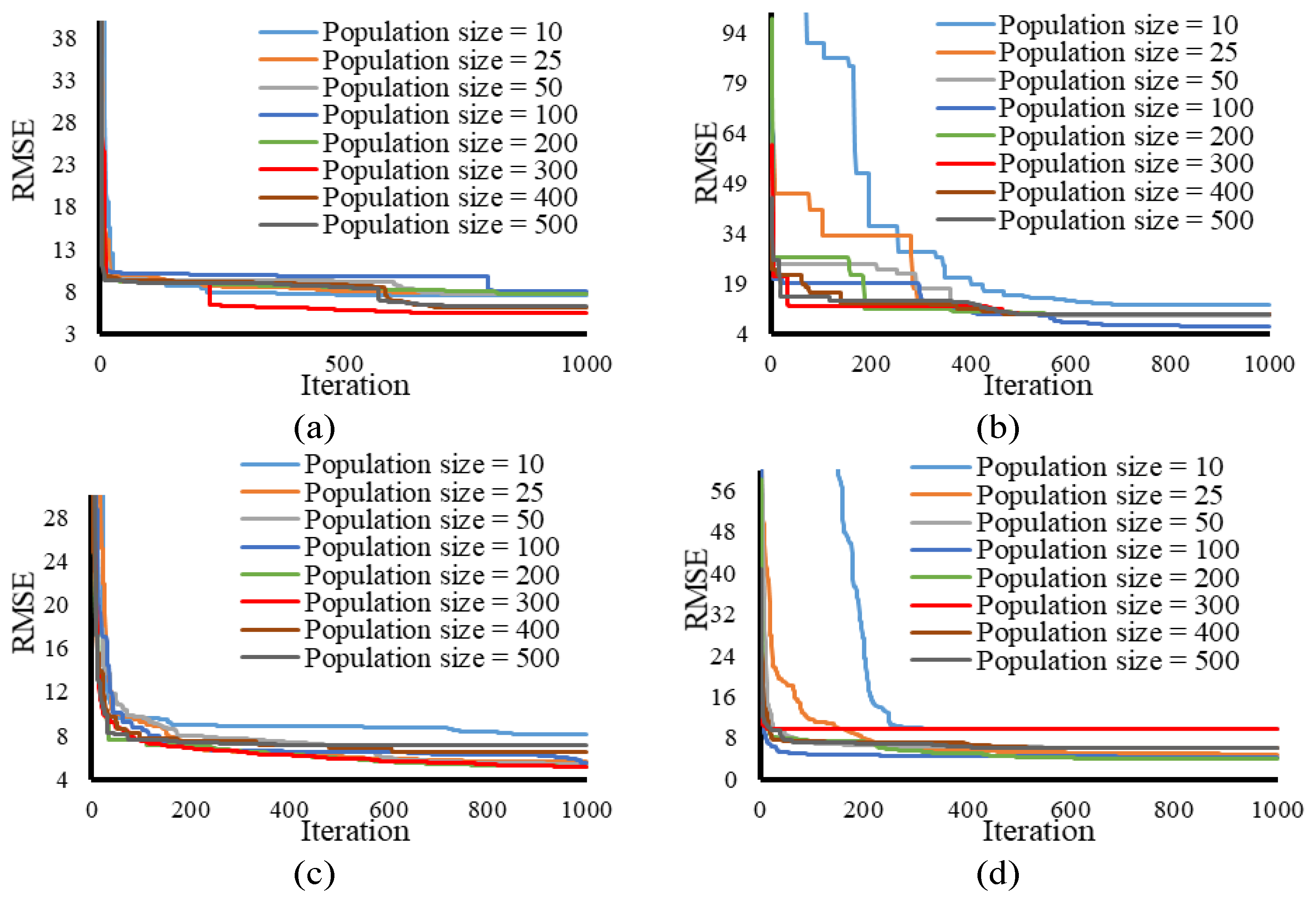
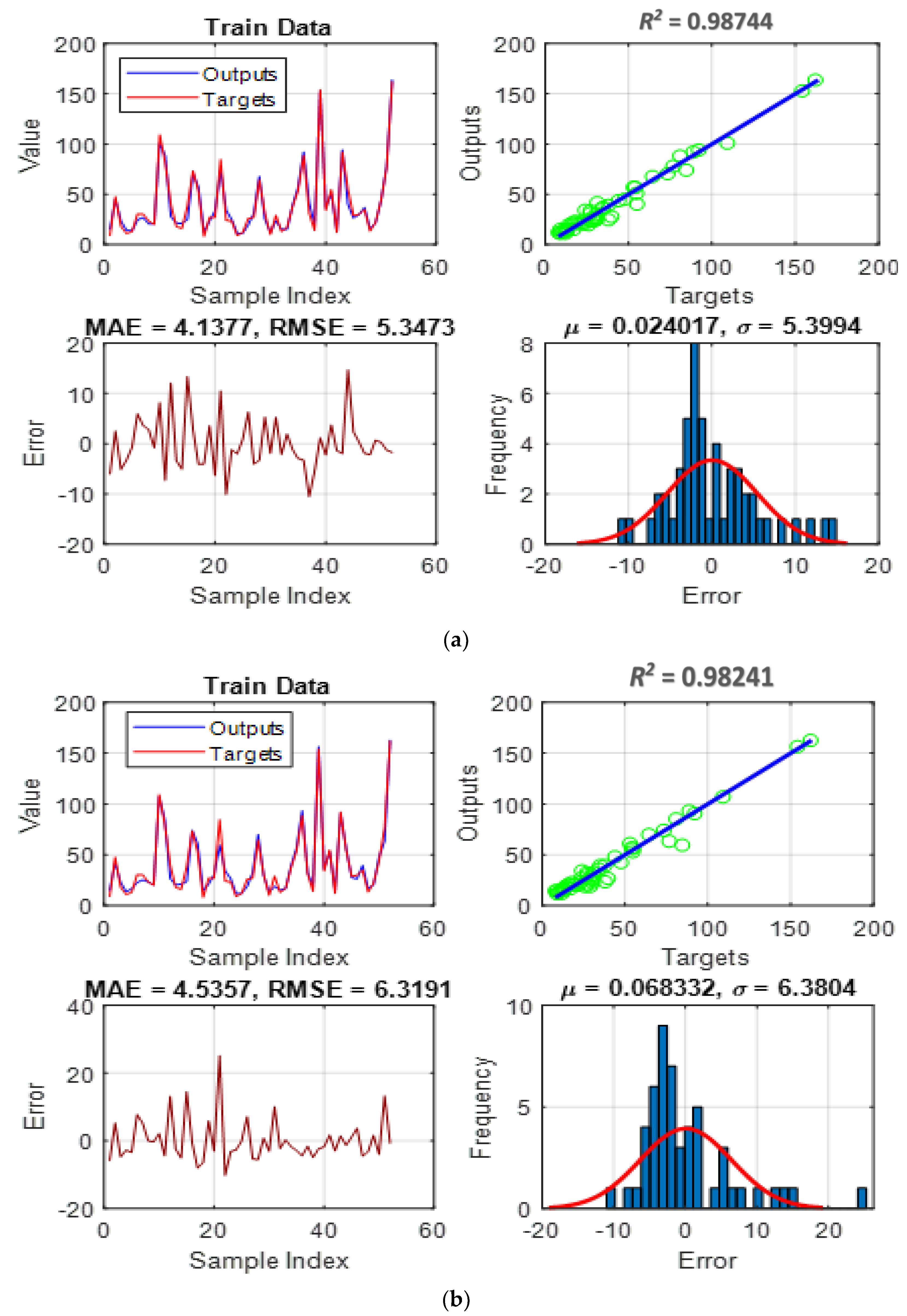
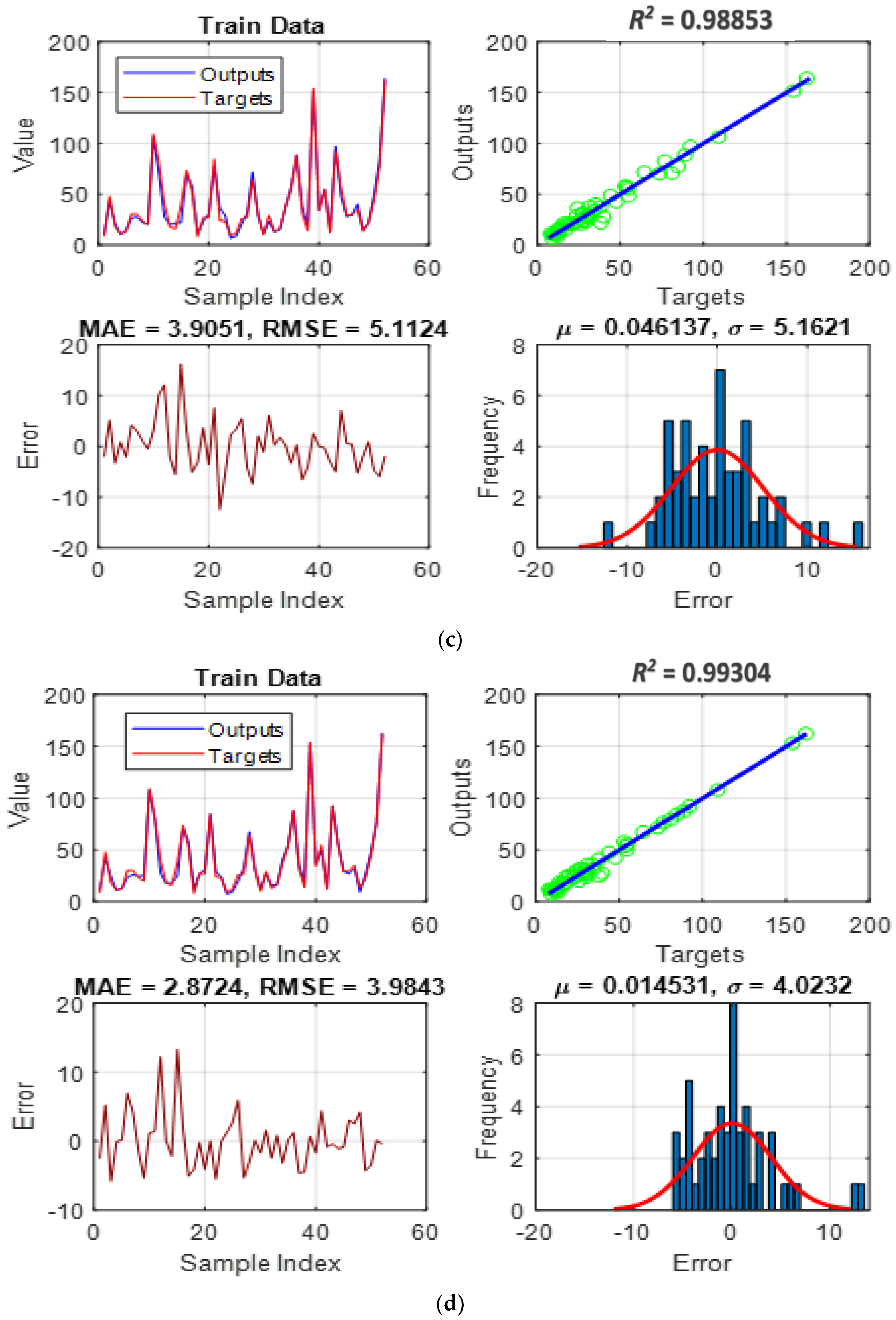
4.1. Developing Hybridized Fuzzy Tools

This section discusses model creation in the MATLAB environment; a random selection with a ratio of 80:20 was applied to the dataset first, containing 52 and 13 samples for the training and testing groups, respectively. Table 2 shows the data for the implemented HHO-ANFIS, SSA-ANFIS, TLBO-ANFIS, and WCA-ANFIS. ANFIS training is achieved through assessing the training samples by changing the parameters of membership functions, and Figure 1 presents the process of realizing an excellent hybridized ANFIS. This was done because each complexity of the assemblage accuracy differs from others and Figure 3a–d gives an account of the convergence process of HHO-ANFIS, SSA-ANFIS, TLBO-ANFIS, and WCA-ANFIS, respectively.
A sum of 1000 iterations was designated for the four assemblages. That means that every proposed hybrid model of HHO, SSA, TLBO, and WCA would update the location of their operator 1000 times. The RMSE changes were controlled by the population sizes (Npops) of 10, 25, 50, 100, 200, 300, 400, and 500. Table 3 shows RMSE of the HHO-ANFIS, SSO-ANFIS, TLBO-ANFIS, and WCA-ANFIS for Npops of 10, 25, 50, 100, 200, 300, 400, and 500, respectively. The best Npops for the HHO-ANFIS, SSO-ANFIS, TLBO-ANFIS, and WCA-ANFIS are 300, 100, 300, and 200, respectively. These population sizes were selected because of their lowest RMSE value in the training phase, as displayed in italic in Table 3. The selected Npop for HHO-ANFIS, SSO-ANFIS, TLBO-ANFIS, and WCA-ANFIS are 300, 100, 300, and 200, respectively. The RMSE starts from 96.9887, 83.9397, 45.4107, and 58.2593, and ends with 5.3473, 6.3191, 5.1124, and 3.9843, respectively. Significant findings could be derived from the graphs in Figure 3, which is their convergence rate when the first 500 iterations of the hybrid algorithm demonstrate the majority of error minimization. The TLBO-ANFIS attains its optimum point much faster than HHO-ANFIS, SSO-ANFIS, and WCA-ANFIS.
The summary of the results from Figure 3 is given in Table 3. Additionally, according to this table, WCA-ANFIS has the lowest RMSE (RMSE = 3.984) related to the population size of 200 and the highest RMSE value is 12.483, related to SSA-ANFIS.

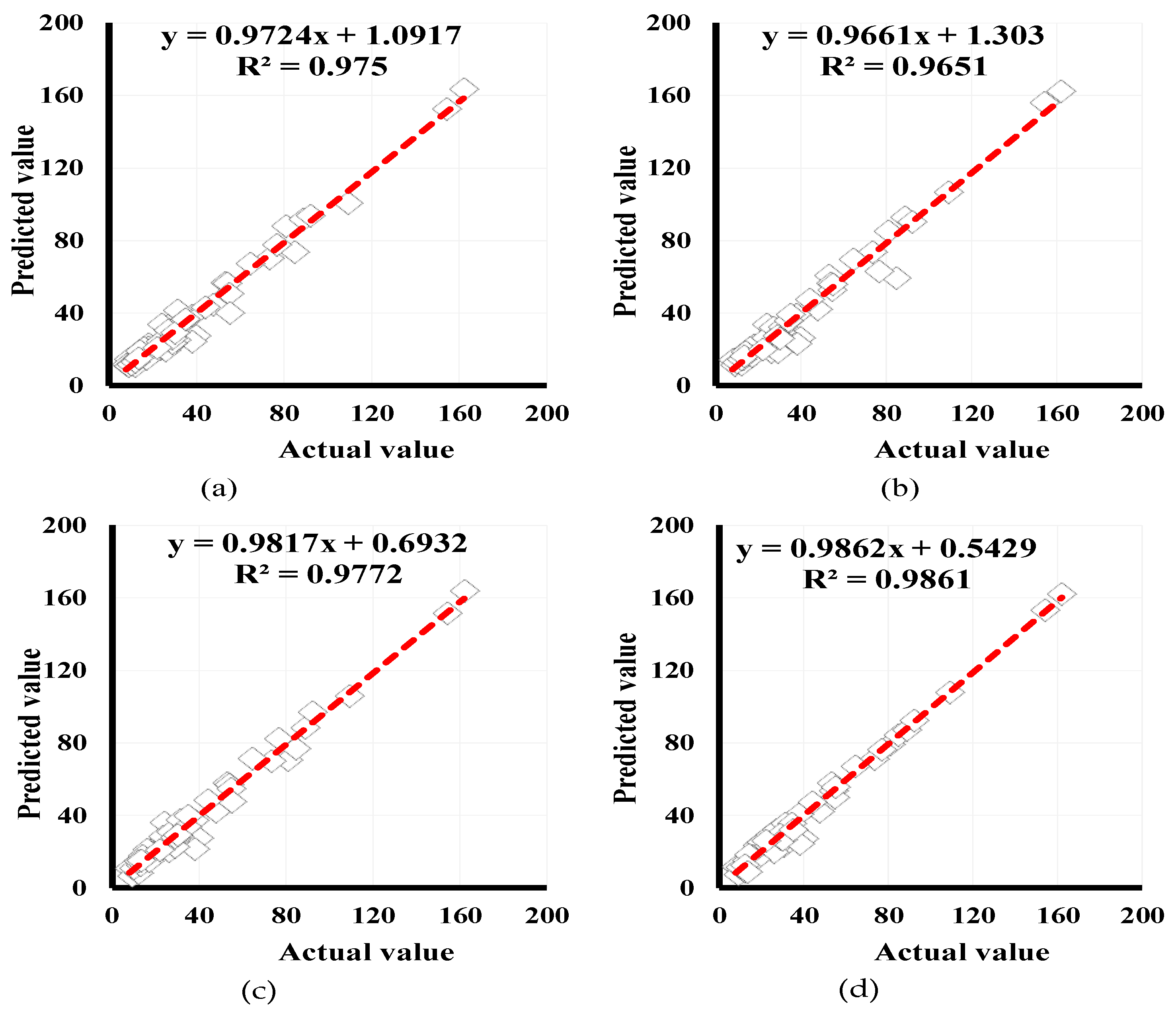
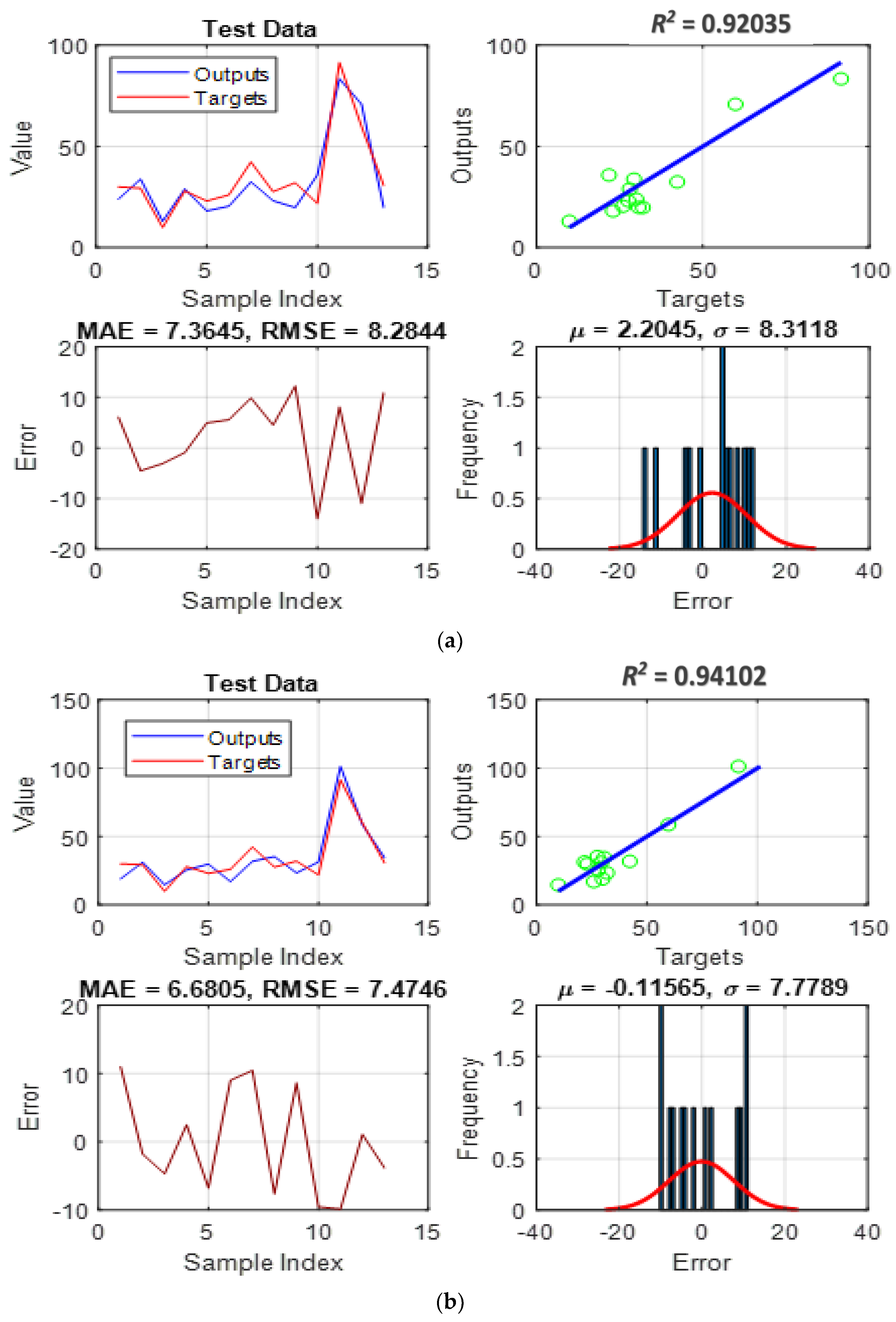
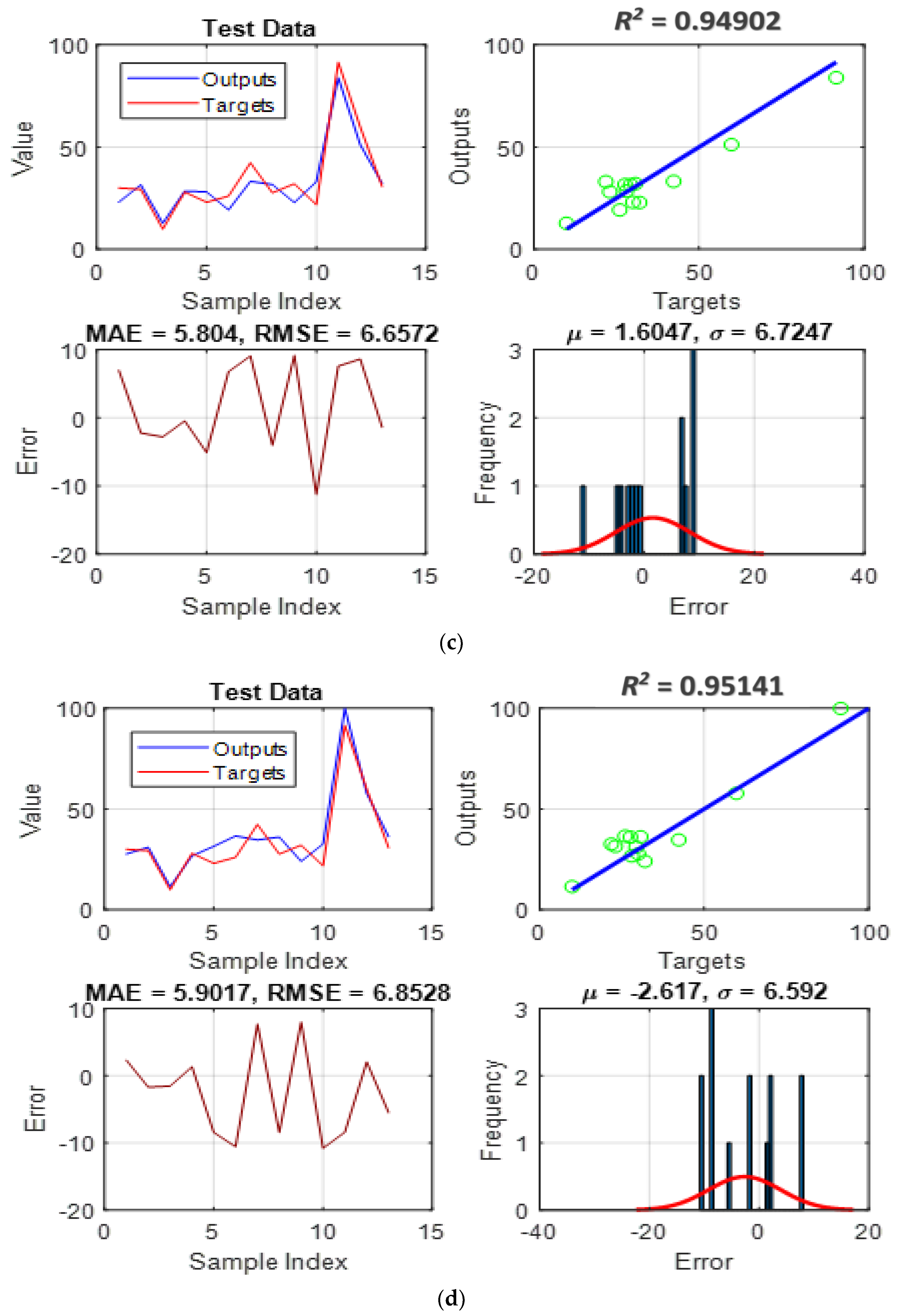
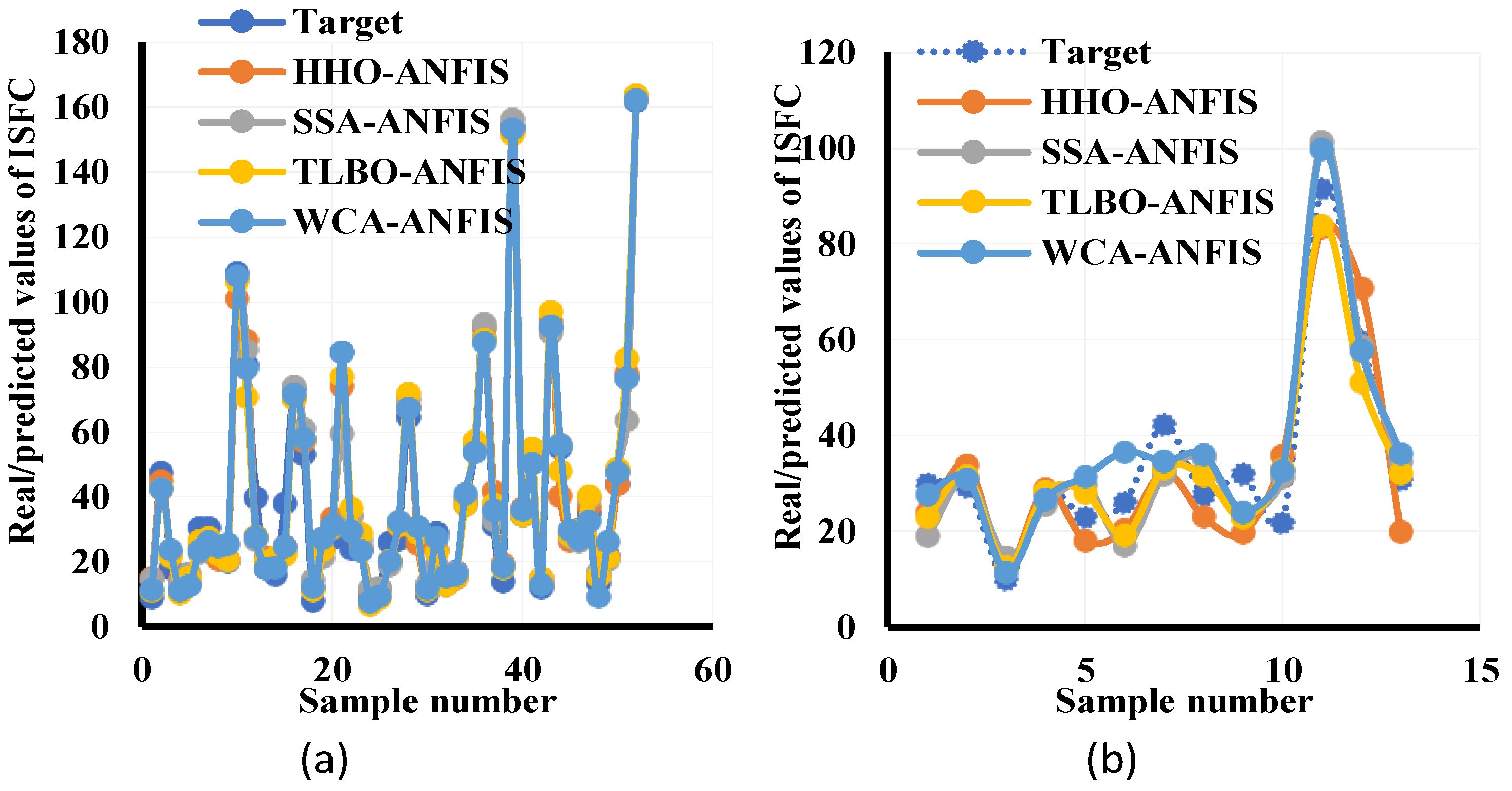
4.2. Simulation and Assessment

The parameters are grouped into training and testing to help in evaluating the model’s two main objectives:
  • Pattern recognition: It provides insight into the question, “How accurately could each model understand the link between pile length, pile diameter, effective vertical stress, and undrained shear strength using the ISFC?” As stated earlier, this task is realized through adjusting the parameters of membership functions that are variables of the ANFIS’s function.
  • Pattern generalization: It responds to the question, “How well can each trained model predict the ISFC under unexpected circumstances?”, the purpose for which testing data is not similar to those utilized in the training phase.
The HHO-ANFIS, SSO-ANFIS, TLBO-ANFIS, and WCA-ANFIS realized the learning RMSE of 5.3473, 6.3191, 5.1124, and 3.9843 with MAE of 4.1377, 4.5357, 3.9051, and 2.8724, respectively. Moreover, Figure 4 exhibits the correlation of the results of the training phase, its mean, and standard deviation. From the previously two indices mentioned above and taking the statistical details of Table 1 into account, all models realize an adequate level of accuracy. However, the higher training veracity of the WCA-ANFIS can be inferred. After taking a closer look at the graphs in Figure 4a–d shows that the ISFCs forecasted by all models correlate outstandingly with expected values. The R2 values of 0.98744, 0.98241, 0.98853, and 0.99304 correlate well with the training results. These proposed models were subsequently integrated into the testing inputs, resulting in an assessment of the ISFC for pile-related scenarios that were previously unknown.
Figure 5a–d shows a relationship between the expected ISFCs and those simulated by the HHO-ANFIS, SSO-ANFIS, TLBO-ANFIS, and WCA-ANFIS predictors for the training phase. These figures demonstrated that all utilized models have befittingly traced the ISFC pattern. The peak of ISFC is 164, estimated by the models as 163.7300, 162.7000, 164.0231, and 162.4016, respectively. Additionally, the values of 97.5%, 96.51%, 97.72%, and 98.61% are obtained for R 2 for which indicates HHO-ANFIS, SSO-ANFIS, TLBO-ANFIS, and WCA-ANFIS models, respectively, which shows the high accuracy prediction of WCA-ANFIS.
Figure 6a–d shows the testing result, and the inaccuracy in the testing phase was indicated by RMSEs of 8.2844, 7.4746, 6.6572, and 6.8528, respectively, with MAEs of 7.3645, 6.6805, 5.8040, and 5.9017 and R value of 0.92035, 0.94102, 0.95902, and 0.95141 for HHO-ANFIS, SSO-ANFIS, TLBO-ANFIS, and WCA-ANFIS models, respectively. These indicate a satisfying accuracy level in predicting the ISFC influenced by four key parameters.
The corresponding correlation charts for the testing results of HHO-ANFIS, SSO-ANFIS, TLBO-ANFIS, and WCA-ANFIS are shown in Figure 7a–d. As shown in these graphs, the outcomes of the HHO-ANFIS, SSO-ANFIS, TLBO-ANFIS, and WCA-ANFIS are 84.71, 88.55, 90.06, and 90.52%, in agreement with the expected values. The fact remains that the utilization of experimental and traditional simulation approaches is costly and time-consuming in predicting the behavior of driven piles [101,102].
Due to the outstanding results given by the TLBO-ANFIS and WCA-ANFIS is deducing and replicating the ISFC pattern. Therefore, these developed methods can be alternatively utilized for practical applications and other related problems. The error of the WCA-ANFIS is lower than that of the other three assemblages, as shown in the accuracy indices obtained in the training phase. Moreover, there are around 0.56, 1.06, and 0.45% differences in R2; therefore, it could be postulated that WCA can train ANFIS more aptly in comparison with HHO, SSA, and TLBO. It is worth noting that WCA-ANFIS featured as an accurate model, followed by the TLBO-ANFIS, SSA-ANFIS, and HHO-ANFIS in the testing phase. Figure 8a–b compares the target ISFC with the model output for training and testing, depicting an almost perfect correlation.

5. Conclusions

The current research aims to evaluate how efficiently several artificial intelligence approaches could measure the friction capacity of driven piles in a cohesive soil environment. Furthermore, as input data, four practical elements that impact the friction capacity of driven piles were studied: length, diameter, effective stress, and undrained cohesion strength of the adjacent soils. The feasibility of the ANFIS system hybridized with HHO, SSA, TLBO, and WCA is used to estimate the ISFC of piles. Driven piles friction capacity prediction cannot be overemphasized in engineering projects. In the same vein, an ANFIS was hybridized with HHO, SSA, TLBO, and WCA to predict the ISFC of driven piles. The lowest value of RMSE and the higher value of R 2 shows the best predictive model. The optimized composition of the four models demonstrated high-quality performances of approximately 97.50, 96.51, 97.72, and 98.61% correlation of training data for the R 2 value. In the case of RMSE, the values of 8.2844, 7.4746, 6.6572, and 6.8528 are obtained for the HHO-ANFIS, SSA-ANFIS, TLBO-ANFIS, and WCA-ANFIS, respectively. This implies proficient dependability for utilizing metaheuristic algorithms in adjusting ANFIS internal parameters. Compared with other models, the solution acquired demonstrated that the WCA-ANFIS is more encouraging in the training and testing phases. The calculated RMSE values for the TLBO-ANFIS-based models were lower than HHO-ANFIS, SSA-ANFIS, and WCA-ANFIS. Irrespective of their level of accuracy, employing the tested models in practical problems is recommended.

Funding

This research received no external funding.

Institutional Review Board Statement

Not applicable.

Informed Consent Statement

Not applicable.

Data Availability Statement

Not applicable.

Conflicts of Interest

The author declare no conflict of interest.

References

  1. Zhao, Y.; Zhong, X.; Foong, L.K. Predicting the splitting tensile strength of concrete using an equilibrium optimization model. Steel and Composite Structures. Int. J. 2021, 39, 81–93. [Google Scholar]
  2. Zhang, Z.; Wang, L.; Zheng, W.; Yin, L.; Hu, R.; Yang, B. Endoscope image mosaic based on pyramid ORB. Biomed. Signal Process. Control. 2022, 71, 103261. [Google Scholar] [CrossRef]
  3. Liu, Y.; Tian, J.; Hu, R.; Yang, B.; Liu, S.; Yin, L.; Zheng, W. Improved Feature Point Pair Purification Algorithm Based on SIFT During Endoscope Image Stitching. Front. Neurorobot. 2022, 16, 840594. [Google Scholar] [CrossRef]
  4. Houssein, E.H.; Mahdy, M.A.; Shebl, D.; Manzoor, A.; Sarkar, R.; Mohamed, W.M. An efficient slime mould algorithm for solving multi-objective optimization problems. Expert Syst. Appl. 2021, 187, 115870. [Google Scholar] [CrossRef]
  5. Petersen, N.C.; Rodrigues, F.; Pereira, F.C. Multi-output bus travel time prediction with convolutional LSTM neural network. Expert Syst. Appl. 2019, 120, 426–435. [Google Scholar] [CrossRef] [Green Version]
  6. JianNai, X.; Shen, B. A novel swarm intelligence optimization approach: Sparrow serach algorithm. Syst. Sci. Control Eng. 2020, 8, 22–34. [Google Scholar]
  7. Seghier, M.E.A.B.; Kechtegar, B.; Amar, M.N.; Correia, J.A.; Trung, N.-T. Simulation of the ultimate conditions of fibre-reinforced polymer confined concrete using hybrid intelligence models. Eng. Fail. Anal. 2021, 128, 105605. [Google Scholar] [CrossRef]
  8. Boussaïd, I.; Lepagnot, J.; Siarry, P. A survey on optimization metaheuristics. Inf. Sci. 2013, 237, 82–117. [Google Scholar] [CrossRef]
  9. Hussain, K.; Salleh, M.N.M.; Cheng, S.; Shi, Y. Metaheuristic research: A comprehensive survey. Artif. Intell. Rev. 2018, 52, 2191–2233. [Google Scholar] [CrossRef] [Green Version]
  10. Abualigah, L.; Diabat, A. Advances in Sine Cosine Algorithm: A comprehensive survey. Artif. Intell. Rev. 2021, 54, 2567–2608. [Google Scholar] [CrossRef]
  11. Sun, G.; Li, C.; Deng, L. An adaptive regeneration framework based on search space adjustment for differential evolution. Neural Comput. Appl. 2021, 33, 9503–9519. [Google Scholar] [CrossRef]
  12. Cabalar, A.F.; Cevik, A.; Gokceoglu, C. Some applications of Adaptive Neuro-Fuzzy Inference System (ANFIS) in geotechnical engineering. Comput. Geotech. 2012, 40, 14–33. [Google Scholar] [CrossRef]
  13. Moayedi, H.; Raftari, M.; Sharifi, A.; Jusoh, W.A.W.; Rashid, A.S.A. Optimization of ANFIS with GA and PSO estimating α ratio in driven piles. Eng. Comput. 2019, 36, 227–238. [Google Scholar] [CrossRef]
  14. Cai, T.; Yu, D.; Liu, H.; Gao, F. Computational Analysis of Variational Inequalities Using Mean Extra-Gradient Approach. Mathematics 2022, 10, 2318. [Google Scholar] [CrossRef]
  15. Shariati, M.; Mafipour, M.S.; Haido, J.H.; Yousif, S.T.; Toghroli, A.; Trung, N.T.; Shariati, A. Identification of the most influencing parameters on the properties of corroded concrete beams using an Adaptive Neuro-Fuzzy Inference System (ANFIS). Steel. Compos. Struct. 2020, 34, 155. [Google Scholar]
  16. Cao, Y.; Babanezhad, M.; Rezakazemi, M.; Shirazian, S. Prediction of fluid pattern in a shear flow on intelligent neural nodes using ANFIS and LBM. Neural Comput. Appl. 2019, 32, 13313–13321. [Google Scholar] [CrossRef]
  17. Armaghani, D.J.; Asteris, P.G. A comparative study of ANN and ANFIS models for the prediction of cement-based mortar materials compressive strength. Neural Comput. Appl. 2020, 33, 4501–4532. [Google Scholar] [CrossRef]
  18. Hussein, A.M. Adaptive Neuro-Fuzzy Inference System of friction factor and heat transfer nanofluid turbulent flow in a heated tube. Case Stud. Therm. Eng. 2016, 8, 94–104. [Google Scholar] [CrossRef] [Green Version]
  19. Esmaeili Falak, M.; Sarkhani Benemaran, R.; Seifi, R. Improvement of the mechanical and durability parameters of construction concrete of the Qotursuyi Spa. Concr. Res. 2020, 13, 119–134. [Google Scholar]
  20. Bayat, S.; Pishkenari, H.N.; Salarieh, H. Observer design for a nano-positioning system using neural, fuzzy and ANFIS networks. Mechatronics 2019, 59, 10–24. [Google Scholar] [CrossRef]
  21. Fathy, A.; Kassem, A.M. Antlion optimizer-ANFIS load frequency control for multi-interconnected plants comprising photovoltaic and wind turbine. ISA Trans. 2018, 87, 282–296. [Google Scholar] [CrossRef] [PubMed]
  22. Fattahi, H.; Hasanipanah, M. An integrated approach of ANFIS-grasshopper optimization algorithm to approximate flyrock distance in mine blasting. Eng. Comput. 2021, 38, 2619–2631. [Google Scholar] [CrossRef]
  23. Sun, G.; Hasanipanah, M.; Amnieh, H.B.; Foong, L.K. Feasibility of indirect measurement of bearing capacity of driven piles based on a computational intelligence technique. Measurement 2020, 156, 107577. [Google Scholar] [CrossRef]
  24. Yu, D. Estimation of pile settlement socketed to rock applying hybrid ALO-ANFIS and GOA-ANFIS approaches. J. Appl. Sci. Eng. 2022, 25, 979–992. [Google Scholar]
  25. Shirazi, A.; Hezarkhani, A.; Pour, A.B.; Shirazy, A.; Hashim, M. Neuro-Fuzzy-AHP (NFAHP) Technique for Copper Exploration Using Advanced Spaceborne Thermal Emission and Reflection Radiometer (ASTER) and Geological Datasets in the Sahlabad Mining Area, East Iran. Remote Sens. 2022, 14, 5562. [Google Scholar] [CrossRef]
  26. Moayedi, H.; Hayati, S. Artificial intelligence design charts for predicting friction capacity of driven pile in clay. Neural Comput. Appl. 2018, 31, 7429–7445. [Google Scholar] [CrossRef]
  27. Mountrakis, G.; Im, J.; Ogole, C. Support vector machines in remote sensing: A review. ISPRS J. Photogramm. Remote Sens. 2011, 66, 247–259. [Google Scholar] [CrossRef]
  28. Yu, J.; Lu, L.; Chen, Y.; Zhu, Y.; Kong, L. An Indirect Eavesdropping Attack of Keystrokes on Touch Screen through Acoustic Sensing. IEEE Trans. Mob. Comput. 2019, 20, 337–351. [Google Scholar] [CrossRef]
  29. Li, P.; Li, Y.; Gao, R.; Xu, C.; Shang, Y. New exploration on bifurcation in fractional-order genetic regulatory networks incorporating both type delays. Eur. Phys. J. Plus 2022, 137, 598. [Google Scholar] [CrossRef]
  30. Prayogo, D.; Susanto, Y.T.T. Optimizing the Prediction Accuracy of Friction Capacity of Driven Piles in Cohesive Soil Using a Novel Self-Tuning Least Squares Support Vector Machine. Adv. Civ. Eng. 2018, 2018, 6490169. [Google Scholar] [CrossRef] [Green Version]
  31. Dehghanbanadaki, A.; Khari, M.; Amiri, S.T.; Armaghani, D.J. Estimation of ultimate bearing capacity of driven piles in c-φ soil using MLP-GWO and ANFIS-GWO models: A comparative study. Soft Comput. 2020, 25, 4103–4119. [Google Scholar] [CrossRef]
  32. Armaghani, D.J.; Harandizadeh, H.; Momeni, E.; Maizir, H.; Zhou, J. An optimized system of GMDH-ANFIS predictive model by ICA for estimating pile bearing capacity. Artif. Intell. Rev. 2021, 55, 2313–2350. [Google Scholar] [CrossRef]
  33. Kumar, M.; Bardhan, A.; Samui, P.; Hu, J.; Kaloop, M. Reliability Analysis of Pile Foundation Using Soft Computing Techniques: A Comparative Study. Processes 2021, 9, 486. [Google Scholar] [CrossRef]
  34. Wang, B.; Moayedi, H.; Nguyen, H.; Foong, L.K.; Rashid, A.S.A. Feasibility of a novel predictive technique based on artificial neural network optimized with particle swarm optimization estimating pullout bearing capacity of helical piles. Eng. Comput. 2019, 36, 1315–1324. [Google Scholar] [CrossRef]
  35. Liang, S.; Foong, L.K.; Lyu, Z. Determination of the friction capacity of driven piles using three sophisticated search schemes. Eng. Comput. 2020, 38, 1515–1527. [Google Scholar] [CrossRef]
  36. Goh, A.T.C. Empirical design in geotechnics using neural networks. Geotechnique 1995, 45, 709–714. [Google Scholar] [CrossRef]
  37. Heidari, A.A.; Mirjalili, S.; Faris, H.; Aljarah, I.; Mafarja, M.; Chen, H. Harris hawks optimization: Algorithm and applications. Futur. Gener. Comput. Syst. 2019, 97, 849–872. [Google Scholar] [CrossRef]
  38. Zhao, Y.; Hu, H.; Song, C.; Wang, Z. Predicting compressive strength of manufactured-sand concrete using conventional and metaheuristic-tuned artificial neural network. Measurement 2022, 194, 110993. [Google Scholar] [CrossRef]
  39. Moayedi, H.; Osouli, A.; Nguyen, H.; Rashid, A.S.A. A novel Harris hawks’ optimization and k-fold cross-validation predicting slope stability. Eng. Comput. 2019, 37, 369–379. [Google Scholar] [CrossRef]
  40. Rodríguez-Esparza, E.; Zanella-Calzada, L.A.; Oliva, D.; Heidari, A.A.; Zaldivar, D.; Pérez-Cisneros, M.; Foong, L.K. An efficient Harris hawks-inspired image segmentation method. Expert Syst. Appl. 2020, 155, 113428. [Google Scholar] [CrossRef]
  41. Qais, M.H.; Hasanien, H.M.; Alghuwainem, S. Parameters extraction of three-diode photovoltaic model using computation and Harris Hawks optimization. Energy 2020, 195, 117040. [Google Scholar] [CrossRef]
  42. Moayedi, H.; Abdullahi, M.M.; Nguyen, H.; Rashid, A.S.A. Comparison of dragonfly algorithm and Harris hawks optimization evolutionary data mining techniques for the assessment of bearing capacity of footings over two-layer foundation soils. Eng. Comput. 2019, 37, 437–447. [Google Scholar] [CrossRef]
  43. Wang, S.; Jia, H.; Liu, Q.; Zheng, R. An improved hybrid Aquila Optimizer and Harris Hawks Optimization for global optimization. Math. Biosci. Eng. 2021, 18, 7076–7109. [Google Scholar] [CrossRef] [PubMed]
  44. Alabool, H.M.; Alarabiat, D.; Abualigah, L.; Heidari, A.A. Harris hawks optimization: A comprehensive review of recent variants and applications. Neural Comput. Appl. 2021, 33, 8939–8980. [Google Scholar] [CrossRef]
  45. Yu, D.; Ma, Z.; Wang, R. Efficient Smart Grid Load Balancing via Fog and Cloud Computing. Math. Probl. Eng. 2022, 2022, 3151249. [Google Scholar] [CrossRef]
  46. Chantar, H.; Thaher, T.; Turabieh, H.; Mafarja, M.; Sheta, A. BHHO-TVS: A Binary Harris Hawks Optimizer with Time-Varying Scheme for Solving Data Classification Problems. Appl. Sci. 2021, 11, 6516. [Google Scholar] [CrossRef]
  47. Zhou, G.; Yang, F.; Xiao, J. Study on Pixel Entanglement Theory for Imagery Classification. IEEE Trans. Geosci. Remote Sens. 2022, 60, 5409518. [Google Scholar] [CrossRef]
  48. Kamboj, V.K.; Nandi, A.; Bhadoria, A.; Sehgal, S. An intensify Harris Hawks optimizer for numerical and engineering optimization problems. Appl. Soft Comput. 2019, 89, 106018. [Google Scholar] [CrossRef]
  49. Kong, H.; Lu, L.; Yu, J.; Chen, Y.; Tang, F. Continuous Authentication Through Finger Gesture Interaction for Smart Homes Using WiFi. IEEE Trans. Mob. Comput. 2020, 20, 3148–3162. [Google Scholar] [CrossRef]
  50. Yin, Q.; Cao, B.; Li, X.; Wang, B.; Zhang, Q.; Wei, X. An Intelligent Optimization Algorithm for Constructing a DNA Storage Code: NOL-HHO. Int. J. Mol. Sci. 2020, 21, 2191. [Google Scholar] [CrossRef] [Green Version]
  51. Qu, C.; He, W.; Peng, X.; Peng, X. Harris Hawks optimization with information exchange. Appl. Math. Model. 2020, 84, 52–75. [Google Scholar] [CrossRef]
  52. Zhang, Y.; Liu, R.; Wang, X.; Chen, H.; Li, C. Boosted binary Harris hawks optimizer and feature selection. Eng. Comput. 2020, 37, 3741–3770. [Google Scholar] [CrossRef]
  53. Menesy, A.S.; Sultan, H.M.; Selim, A.; Ashmawy, M.G.; Kamel, S. Developing and Applying Chaotic Harris Hawks Optimization Technique for Extracting Parameters of Several Proton Exchange Membrane Fuel Cell Stacks. IEEE Access 2019, 8, 1146–1159. [Google Scholar] [CrossRef]
  54. Chen, H.; Jiao, S.; Wang, M.; Heidari, A.A.; Zhao, X. Parameters identification of photovoltaic cells and modules using diversification-enriched Harris hawks optimization with chaotic drifts. J. Clean. Prod. 2019, 244, 118778. [Google Scholar] [CrossRef]
  55. Moayedi, H.; Gör, M.; Lyu, Z.; Bui, D.T. Herding Behaviors of grasshopper and Harris hawk for hybridizing the neural network in predicting the soil compression coefficient. Measurement 2019, 152, 107389. [Google Scholar] [CrossRef]
  56. Wei, Y.; Lv, H.; Chen, M.; Wang, M.; Heidari, A.A.; Chen, H.; Li, C. Predicting Entrepreneurial Intention of Students: An Extreme Learning Machine with Gaussian Barebone Harris Hawks Optimizer. IEEE Access 2020, 8, 76841–76855. [Google Scholar] [CrossRef]
  57. Mirjalili, S.; Gandomi, A.H.; Mirjalili, S.Z.; Saremi, S.; Faris, H.; Mirjalili, S.M. Salp Swarm Algorithm: A bio-inspired optimizer for engineering design problems. Adv. Eng. Softw. 2017, 114, 163–191. [Google Scholar] [CrossRef]
  58. Abualigah, L.; Shehab, M.; Alshinwan, M.; Alabool, H. Salp swarm algorithm: A comprehensive survey. Neural Comput. Appl. 2020, 32, 11195–11215. [Google Scholar] [CrossRef]
  59. Liu, L.; Xiang, H.; Li, X. A novel perturbation method to reduce the dynamical degradation of digital chaotic maps. Nonlinear Dyn. 2021, 103, 1099–1115. [Google Scholar] [CrossRef]
  60. Rao, R.V.; Savsani, V.J.; Vakharia, D.P. Teaching–learning-based optimization: A novel method for constrained mechanical design optimization problems. Comput. Aided Des. 2011, 43, 303–315. [Google Scholar] [CrossRef]
  61. Rao, R.; Savsani, V.; Vakharia, D. Teaching–Learning-Based Optimization: An optimization method for continuous non-linear large scale problems. Inf. Sci. 2012, 183, 1–15. [Google Scholar] [CrossRef]
  62. Niknam, T.; Azizipanah-Abarghooee, R.; Narimani, M.R. A new multi objective optimization approach based on TLBO for location of automatic voltage regulators in distribution systems. Eng. Appl. Artif. Intell. 2012, 25, 1577–1588. [Google Scholar] [CrossRef]
  63. Tang, Y.; Liu, S.; Deng, Y.; Zhang, Y.; Yin, L.; Zheng, W. An improved method for soft tissue modeling. Biomed. Signal Process. Control. 2021, 65, 102367. [Google Scholar] [CrossRef]
  64. Chen, X.; Mei, C.; Xu, B.; Yu, K.; Huang, X. Quadratic interpolation based teaching-learning-based optimization for chemical dynamic system optimization. Knowl. Based Syst. 2018, 145, 250–263. [Google Scholar] [CrossRef]
  65. Chen, X.; Xu, B.; Yu, K.; Du, W. Teaching-Learning-Based Optimization with Learning Enthusiasm Mechanism and Its Application in Chemical Engineering. J. Appl. Math. 2018, 2018, 1806947. [Google Scholar] [CrossRef]
  66. Zhao, Y.; Moayedi, H.; Bahiraei, M.; Foong, L.K. Employing TLBO and SCE for optimal prediction of the compressive strength of concrete. Smart Struct. Syst. 2020, 26, 753–763. [Google Scholar]
  67. Eskandar, H.; Sadollah, A.; Bahreininejad, A.; Hamdi, M. Water cycle algorithm–A novel metaheuristic optimization method for solving constrained engineering optimization problems. Comput. Struct. 2012, 110, 151–166. [Google Scholar] [CrossRef]
  68. Mafarja, M.; Abdullah, S. Fuzzy Modified Great Deluge Algorithm for Attribute Reduction. In Recent Advances on Soft Computing and Data Mining; Springer Nature: Cham, Switzerland AG, 2014; pp. 195–203. [Google Scholar] [CrossRef]
  69. Mafarja, M.; Abdullah, S. A fuzzy record-to-record travel algorithm for solving rough set attribute reduction. Int. J. Syst. Sci. 2013, 46, 503–512. [Google Scholar] [CrossRef]
  70. Foong, L.K.; Zhao, Y.; Bai, C.; Xu, C. Efficient metaheuristic-retrofitted techniques for concrete slump simulation. Smart Struct. Syst. Int. J. 2021, 27, 745–759. [Google Scholar]
  71. Mosallanezhad, M.; Moayedi, H. Developing hybrid artificial neural network model for predicting uplift resistance of screw piles. Arab. J. Geosci. 2017, 10, 479. [Google Scholar] [CrossRef]
  72. Yu, D.; Wu, J.; Wang, W.; Gu, B. Optimal performance of hybrid energy system in the presence of electrical and heat storage systems under uncertainties using stochastic p-robust optimization technique. Sustain. Cities Soc. 2022, 83, 103935. [Google Scholar] [CrossRef]
  73. Mou, J.; Duan, P.; Gao, L.; Liu, X.; Li, J. An effective hybrid collaborative algorithm for energy-efficient distributed permutation flow-shop inverse scheduling. Futur. Gener. Comput. Syst. 2021, 128, 521–537. [Google Scholar] [CrossRef]
  74. Lu, C.; Liu, Q.; Zhang, B.; Yin, L. A Pareto-based hybrid iterated greedy algorithm for energy-efficient scheduling of distributed hybrid flowshop. Expert Syst. Appl. 2022, 204, 117555. [Google Scholar] [CrossRef]
  75. Seghier, M.E.A.B.; Ouaer, H.; Ghriga, M.A.; Menad, N.A.; Thai, D.-K. Hybrid soft computational approaches for modeling the maximum ultimate bond strength between the corroded steel reinforcement and surrounding concrete. Neural Comput. Appl. 2020, 33, 6905–6920. [Google Scholar] [CrossRef]
  76. Moayedi, H.; Mosavi, A. A water cycle-based error minimization technique in predicting the bearing capacity of shallow foundation. Eng. Comput. 2021, 1–14. [Google Scholar] [CrossRef]
  77. Yan, L.; Yin-He, S.; Qian, Y.; Zhi-Yu, S.; Chun-Zi, W.; Zi-Yun, L. Method of Reaching Consensus on Probability of Food Safety Based on the Integration of Finite Credible Data on Block Chain. IEEE Access 2021, 9, 123764–123776. [Google Scholar] [CrossRef]
  78. Foong, L.K.; Moayedi, H.; Lyu, Z. Computational modification of neural systems using a novel stochastic search scheme, namely evaporation rate-based water cycle algorithm: An application in geotechnical issues. Eng. Comput. 2020, 37, 3347–3358. [Google Scholar] [CrossRef]
  79. Nasir, M.; Sadollah, A.; Choi, Y.H.; Kim, J.H. A comprehensive review on water cycle algorithm and its applications. Neural Comput. Appl. 2020, 32, 17433–17488. [Google Scholar] [CrossRef]
  80. Eskandar, H.; Sadollah, A.; Bahreininejad, A. Weight optimization of truss structures using water cycle algorithm. Iran Univ. Sci. Technol. 2013, 3, 115–129. [Google Scholar]
  81. Haddad, O.B.; Moravej, M.; Loáiciga, H.A. Application of the Water Cycle Algorithm to the Optimal Operation of Reservoir Systems. J. Irrig. Drain. Eng. 2015, 141, 04014064. [Google Scholar] [CrossRef]
  82. Jabbar, A.; Zainudin, S. Water cycle algorithm for attribute reduction problems in rough set theory. J. Theor. Appl. Inf. Technol. 2014, 61, 107–117. [Google Scholar]
  83. Roeva, O.; Angelova, M.; Zoteva, D.; Pencheva, T. Water Cycle Algorithm for Modelling of Fermentation Processes. Processes 2020, 8, 920. [Google Scholar] [CrossRef]
  84. Sadollah, A.; Yoo, D.G.; Yazdi, J.; Kim, J.H.; Choi, Y. Application of water cycle algorithm for optimal cost design of water distribution systems. In Proceedings of the 11th International Conference on Hydroinformatics, New York, NY, USA, 16–20 August 2014. [Google Scholar]
  85. Sadollah, A.; Eskandar, H.; Bahreininejad, A.; Kim, J.H. Water cycle, mine blast and improved mine blast algorithms for discrete sizing optimization of truss structures. Comput. Struct. 2014, 149, 1–16. [Google Scholar] [CrossRef]
  86. Zhong, L.; Fang, Z.; Liu, F.; Yuan, B.; Zhang, G.; Lu, J. Bridging the Theoretical Bound and Deep Algorithms for Open Set Domain Adaptation. IEEE Trans. Neural Networks Learn. Syst. 2021, 32, 1–15. [Google Scholar] [CrossRef] [PubMed]
  87. Zhang, Y.; Liu, F.; Fang, Z.; Yuan, B.; Zhang, G.; Lu, J. Learning from a Complementary-Label Source Domain: Theory and Algorithms. IEEE Trans. Neural Networks Learn. Syst. 2021, 32, 7667–7681. [Google Scholar] [CrossRef] [PubMed]
  88. Liu, K.; Ke, F.; Huang, X.; Yu, R.; Lin, F.; Wu, Y.; Ng, D.W.K. DeepBAN: A Temporal Convolution-Based Communication Framework for Dynamic WBANs. IEEE Trans. Commun. 2021, 69, 6675–6690. [Google Scholar] [CrossRef]
  89. Xie, Y.; Sheng, Y.; Qiu, M.; Gui, F. An adaptive decoding biased random key genetic algorithm for cloud workflow scheduling. Eng. Appl. Artif. Intell. 2022, 112, 104879. [Google Scholar] [CrossRef]
  90. Goh, A.T.C. Pile Driving Records Reanalyzed Using Neural Networks. J. Geotech. Eng. 1996, 122, 492–495. [Google Scholar] [CrossRef]
  91. Jang, J.-S.R. ANFIS: Adaptive-Network-Based Fuzzy Inference System. IEEE Trans. Syst. Man Cybern. 1993, 23, 665–685. [Google Scholar] [CrossRef]
  92. Zhao, L.; Wang, L. A new lightweight network based on MobileNetV3. KSII Trans. Internet Inf. Syst. 2022, 16, 1–15. [Google Scholar]
  93. Meng, Q.; Lai, X.; Yan, Z.; Su, C.-Y.; Wu, M. Motion Planning and Adaptive Neural Tracking Control of an Uncertain Two-Link Rigid–Flexible Manipulator with Vibration Amplitude Constraint. IEEE Trans. Neural Networks Learn. Syst. 2021, 33, 3814–3828. [Google Scholar] [CrossRef] [PubMed]
  94. Liang, X.; Luo, L.; Hu, S.; Li, Y. Mapping the knowledge frontiers and evolution of decision making based on agent-based modeling. Knowledge-Based Syst. 2022, 250, 108982. [Google Scholar] [CrossRef]
  95. Zhao, Y.; Wang, Z. Subset simulation with adaptable intermediate failure probability for robust reliability analysis: An unsupervised learning-based approach. Struct. Multidiscip. Optim. 2022, 65, 172. [Google Scholar] [CrossRef]
  96. Seghier, M.E.A.B.; Gao, X.-Z.; Jafari-Asl, J.; Thai, D.-K.; Ohadi, S.; Trung, N.-T. Modeling the nonlinear behavior of ACC for SCFST columns using experimental-data and a novel evolutionary-algorithm. Structures 2021, 30, 692–709. [Google Scholar] [CrossRef]
  97. Zhu, H.; Xue, M.; Wang, Y.; Yuan, G.; Li, X. Fast Visual Tracking with Siamese Oriented Region Proposal Network. IEEE Signal Process. Lett. 2022, 29, 1437–1441. [Google Scholar] [CrossRef]
  98. Razavi-Termeh, S.V.; Shirani, K.; Pasandi, M. Mapping of landslide susceptibility using the combination of neuro-fuzzy inference system (ANFIS), ant colony (ANFIS-ACOR), and differential evolution (ANFIS-DE) models. Bull. Eng. Geol. Environ. 2021, 80, 2045–2067. [Google Scholar] [CrossRef]
  99. Chen, Y.K.; Weng, S.X.; Liu, T.P. Teaching–learning based optimization (TLBO) with variable neighborhood search to retail shelf-space allocation. Mathematics 2020, 8, 1296. [Google Scholar] [CrossRef]
  100. Gill, H.S.; Khehra, B.S.; Singh, A.; Kaur, L. Teaching-learning-based optimization algorithm to minimize cross entropy for selecting multilevel threshold values. Egypt. Inform. J. 2019, 20, 11–25. [Google Scholar] [CrossRef]
  101. Moayedi, H.; Armaghani, D.J. Optimizing an ANN model with ICA for estimating bearing capacity of driven pile in cohesionless soil. Eng. Comput. 2017, 34, 347–356. [Google Scholar] [CrossRef]
  102. Moayedi, H.; Hayati, S. Applicability of a CPT-based neural network solution in predicting load-settlement responses of bored pile. Int. J. Geomech. 2018, 18, 06018009. [Google Scholar] [CrossRef]
Figure 1. Graphical input and output data layers, (a) pile length (m), (b) pile diameter (cm), (c) vertical effective stress (kPa), (d) undrained shear strength (kPa), and (e) friction capacity of driven piles (kPa).
Geotechnics 02 00049 g001
Figure 2. The optimization scheme using the HHO, SSA, TLBO, and WCA.
Geotechnics 02 00049 g002
Figure 3. The trial and error-based optimization of the (a) HHO–ANFIS, (b) SSA–ANFIS, (c) TLBO–ANFIS, and (d) WCA–ANFIS.
Geotechnics 02 00049 g003
Figure 4. Training results of the (a) HHO–ANFIS, (b) SSA–ANFIS, (c) TLBO–ANFIS, and (d) WCA–ANFIS.
Geotechnics 02 00049 g004aGeotechnics 02 00049 g004b
Figure 5. Correlation charts for the training results of (a) HHO–ANFIS, (b) SSO–ANFIS, (c) TLBO–ANFIS, and (d) WCA–ANFIS.
Geotechnics 02 00049 g005
Figure 6. Testing results of the (a) HHO–ANFIS, (b) SSA–ANFIS, (c) TLBO–ANFIS, and (d) WCA–ANFIS.
Geotechnics 02 00049 g006aGeotechnics 02 00049 g006b
Figure 7. Correlation charts for the testing results of (a) HHO–ANFIS, (b) SSO–ANFIS, (c) TLBO–ANFIS, and (d) WCA–ANFIS.
Geotechnics 02 00049 g007
Figure 8. Target ISFC comparison with simulated for (a) ISFC training and (b) ISFC testing.
Geotechnics 02 00049 g008
Table 1. Statistics calculated for the dataset.
ParameterStatistics
AverageStandard DeviationSample VarianceMinimumMaximum
pile length (m)21.116.5271.63.596.0
pile diameter (cm)31.516.6275.311.476.7
vertical effective stress (kPa)124.6127.716,309.919.0718.0
undrained shear strength (kPa)62.260.03603.69.0335.0
in situ friction capacity (ISFC) (kPa)39.331.91014.88.0162.0
Table 2. Parameters of the implemented algorithms.
HHO-ANFISSSA-ANFISTLBO-ANFISWCA-ANFIS
Npops = 300Npops =100Npops = 300Npops = 200
Iteration = 1000Iteration = 1000Iteration = 1000Iteration = 1000
Nsr = 4
dmax = 1.0 × 10⁻⁶
Table 3. The training RMSE of the tested swarm sizes.
Population SizesHHO-ANFISSSA-ANFISTLBO-ANFISWCA-ANFIS
107.47212.4838.0779.656
257.7959.7155.6454.808
507.7479.1865.3416.042
1008.0216.3195.5454.292
2007.6799.7055.1403.984
3005.3479.7055.1129.705
4006.0939.7056.5526.129
5006.1989.7057.0545.987
Publisher’s Note: MDPI stays neutral with regard to jurisdictional claims in published maps and institutional affiliations.

