Finite Element Simulations of Fluids Leakage through the Faulted Reservoir

Abstract

Carbon dioxide (CO₂) capture and storage (CCS) in geological formation as a supercritical fluid is a viable option to reduce anthropogenic greenhouse gas emissions. Due to the density difference between CO₂ and formation fluid, CO₂ shows a buoyant tendency. Thereby, if CO₂ migrates towards the fault in a compromised faulted reservoir, it may escape the storage reservoir. Therefore, it is essential to predict fluids leakage through the faulted reservoir into the aquifer, associated pressure development, and fluids properties over time to assess associated risk and quantification of leakage. We present finite element simulations of miscible fluids flow through the faulted reservoir to elucidate this behavior. There are very few attempts to model multicomponent fluids non-isothermal model during phase change including the Equation of State (EoS) which we addressed by coupling the mass balance equation of fluids, the fractional mass transport, and the energy balance equation. To obtain fluids mixture thermo-physical properties, we used the Peng-Robinson EoS. For validation of the coupled formulation, we compared the simulation results with Ketzin Pilot project field monitoring data, which shows good agreement. A faulted reservoir comprised of five layers is used to investigate fluids leakage through a compromised reservoir. These layers are a CO₂ storage reservoir, overlain by alternating caprocks and aquifers. We also considered three different CO₂ injection rates to study the injection rate effect to assess the pressure buildup during injection process. We present the thermal effect by comparing the isothermal and the non-isothermal conditions. For the latter case, we assumed three different thermal gradients. Additionally, to assess the fault aperture effect, we studied three different apertures. We observed that developed pressure and fluids properties have effects on injection rates, temperature gradient, and fault aperture. Additionally, such responses in the near-field and the far-field from the injection well are critical to assess the risk, which we discussed in this paper.

1. Introduction

After the industrial revolution in 1750, the amount of greenhouse gases (GHG) increases that trap and holds energy from solar radiation in the earth’s atmosphere in the form of heat, have contributed to a gradual rise in mean atmospheric temperature. Among these greenhouse gasses, carbon dioxide (CO₂) emitted from large-scale combustion of fossil fuels is seen as a primary contributor to this effect (Bachu [1]; Volk [2]; EPA [3]; Metz et al. [4]). After 1990, GHG in the United States increased by 3.5% while the contribution of CO₂ was 82.2%, and CO₂ concentration is increasing [5]. In this regard, Eggleton [6] reported that the global amount of CO₂ increased by 45% after the industrial revolution. Bruckner et al. [7] presented that the estimated CO₂ emission from the energy section in 2010 was 14.4 GtCO₂/year and is projected to increase by 25 to 30 GtCO₂/year by 2050. To offset anticipated future increases in emissions, the capture of CO₂ emissions from large anthropogenic point sources, utilization, and long-term, safe geologic storage (CCUS) is being actively considered as a means to manage and reduce atmospheric CO₂ concentrations.

The essential steps in CCUS are separation of CO₂, compression to a dense-phase fluid, transportation from the location of separation to the point of disposal, and injection into deep geologic formations for long term storage. Several candidate geologic storage targets are described in the scientific and industry literature (see also Nordbotten and Celia [8]). These include depleted oil and gas reservoirs, coal seams, and deep saline formations as the most prospective storage options, with basalt formations and unconventional organic-rich shale formations have also been considered (see also NETL [9]).

Viable storage targets will have a storage interval with sufficient injectivity and capacity to store large volumes of CO₂, an injection depth sufficient to ensure that CO₂ is stored in dense fluid phase (liquid or supercritical fluid; nominally 800 m) (Rutqvist and Tsang [10]; Benson and Cole [11]), and a laterally extensive caprock sequence above the storage interval capable of preventing unwanted vertical fluid migration. Bouyance of the stored CO₂ relative to the connate fluid (e.g., brine) and elevated pressure of the storage reservoir in response to large-scale CO₂ injection are driving forces for potential unwanted migration of CO₂ and brine into overlying receptors of concern (groundwater formations and the atmosphere). Geomechanical, thermal, and geochemical phenomena also influence storage system performance.

To capture the full complexity of the dynamics of geologic carbon storage systems requires coupled simulation of fluid flow, energy, and fractional mass transport. This is the motivation for model formulation in this study. Presence of a fault through an impermeable caprock presents a potential pathway for fluid migration that could potentially impact the containment of CO₂ [12]. Consideration of the potential of faults to leak fluids flow behavior through the faulted reservoir during and after the CO₂ injection in the storage reservoir considering the thermodynamics of fluids, which is the point of interest to study the fluids migration behavior.

The finite element (FE) modeling of multicomponent fluids (e.g., gas and liquid) mixture properties (e.g., density, viscosity) change is challenging during change of pressure and temperature. For example, fluids temperature and pressure in a CO₂ storage tank is different than the storage reservoir. Therefore, the bottom hole pressure suddenly increases due to the fluid volume expansion for temperature variation. Additionally, the accuracy of results and numerical convergence conditions in FE solutions are important (Helmig [13]). A similar intricacy also involved in enhanced oil and gas recovery, bio-mechanics and hazardous waste disposal projects, where fluids flow through a porous media and non-isothermal condition exist in the phase transition process. For such a case, it is important to introduce the equations of state (EoS) in the governing process of the model formulation. The isothermal study of fluids and the non-isothermal study of a single fluid are well documented in the literature (Bear and Bachmat [14]). However, there are very few attempts to model multicomponent fluids non-isothermal model during phase change including the EoS. The reduced order models (ROM) are most popular to address a case-specific problem (Vasylkivska et al. [15]). Among others, Rutqvist and his co-workers [10,16] also coupled FLAC and TOUGH for CO₂ sequestration applications. Rutqvist [16] reported the method as a ‘pragmatic approach’. In this regard, Beck et al. [17] presented that node sharing in finite difference approach to achieve a solution of two different codes may results accuracy issues during incremental time steps. There are few literatures where coupled FE solutions are available showing an industry scale verification representing the accuracy of the results. To address such a challenge, we presented a couple FE model formulation, validation and application in this paper.

In this paper, we present a finite element simulation that couples the fluid mass balance equation, the energy balance equation, and the fractional mass transport. We also use the Helmholtz free energy (Wagner and Pruß [18]) for two fluids: carbon dioxide and water, and the Peng-Robinson Equation of State (EoS) (Peng and Robinson [19]) to describe the thermo-physical properties of fluid mixtures. A comparison of the field monitoring measured pressure response of the Ketzin CCUS project (see Kempka and Kühn [20]) with simulated pressure using a version of the model developed herein tuned to Ketzin project geologic and injection data from literature and TOUGH (Pruess [21]) provides validation of our modeling approach.

We present a coupled finite element model to address fluids flow through the faulted reservoir. The study domain is comprised of a CO₂ storage reservoir, aquifers, and caprocks. To ensure the supercritical CO₂, we also assumed that the model domain’s top surface is located 1000 m below the ground surface and considered miscibility of aqueous and CO₂-rich phases. A constant fault aperture is assumed and potential fault propagation is not considered assuming the parallel plate theory [22]. The model captures pressure evolution with CO₂ injection and distribution of fluids mole fraction (e.g., CO₂, H₂O) (see

Table A1. Constants for CO₂ and H₂O.

Fluids	${\mathit{\rho }}_{\mathit{c}}$	${\mathit{T}}_{\mathit{c}}$	${\mathit{p}}_{\mathit{c}}$	$\mathit{\omega }$	$\mathit{M}$
	Kg/m3	K	Pa	-	kg/kmol
CO2	467.6	304.13	7,377,300	0.22491	44.01
H2O	322	647.096	22,064,000	0.344	18.015

, Figure A1 and Figure A2). To reduce the computational time, we considered a simplified geometry and 300 days of simulated site performance.

The following sections present detail of the numerical model, finite element implementation, benchmark validation, and application of the model to capture fluid flow behavior through the faulted reservoir.

2. Governing Equations

The composite medium in the model represents fluid-filled porous rock, so is comprised of fluids phase (f) and solid phase (s). The fluid phase is consisting water (H₂O) and carbon dioxide (CO₂), with pore spaces in the solid-phase represented as macropore (inter-aggregate, e.g., fracture) and micropore (intra-aggregate, e.g., solid matrix) following the dual porosity conceptualization presented by Wilson and Aifantis [23]. The mobility of fluids depends on their physical disposition relative to those pores (i.e., fluids in macropores are mobile or relatively mobile while fluids in micropores are immobile). We obtain such a dual porosity concept following the macroscopic continuum method and using the Representative Elementary Volume (REV) and satisfying the inequality (see also Bear and Bachmat [14]). When fluids are composed of more than one species and their flow accompanies its transport, the governing equations require both the mass balance equation and the fractional mass transport equation (Hassanizadeh [24]; Bear and Bachmat [14]). In the following section, we discuss both of them and the energy balance.

We assumed that (i) the porous media is non-deformable considering solid domain and fluid pressure, (ii) fluid constituents are miscible and satisfy the local thermodynamics equilibrium condition, (iii) fluid phases obey the Darcy’s law which complies with the Reynolds number and (iv) fluid composition is governed with respect to its mass fraction (Bear and Bachmat [14]).

Considering the above assumptions and Hassanizadeh [24]; Bear and Bachmat [14], the balance equations are present as follows:

2.1. Kinematics

Truesdell and Noll [25] presented suppositions which, also known as the “metaphysical principles” to describe the continuum mechanics of a single constituent to many constituents, i.e., mixtures. Atkin and Craine [26]; Bowen [27] also illustrated reviews of the continuum theory of mixtures. The mixture can be homogeneous (e.g., miscible fluids, like soluble salt in water) or heterogeneous (e.g., immiscible fluids or fluid-solid, like, water-sand) which are also state-dependent, and one may obtain exceptions by changing the physical conditions, e.g., temperature. CO₂ injection in a brine or water saturated storage reservoir presents a case in which (i) fluids may be miscible or immiscible depending on the state variables and (ii) the body may be deformable or non-deformable considering fluid flow in a porous media and associated initial and boundary conditions. In this paper, we limited our discussion to the miscible case and relative rigid body, while in Islam et al. [28], we presented a coupled formulation for the immiscible case and deformable body. Moreover, in Islam and Gnanendran [29] and Islam et al. [30], we also discussed elasto-viscoplastic solutions of the material body considering the creep and relaxation based on the two-phases theory, i.e., solid and fluid couple.

In this section, we defined “point” and “particle” as a specific location in a particular space and material point, i.e., a volumetric element), respectively. Assuming a domain, $\Omega \subset {\Re }^d;d=1, 2, 3$ composed of $N$ continuous bodies, while at any reference time $\left(t=0\right)$, each continuous body comprises particles and their constituents. We present the configuration of a continuum body, where the position vector at $t=0$ and $t=t$ are $\mathit{X}={\mathit{X}}_k{\widehat{\mathit{I}}}_k$ and $\mathit{x}={\mathit{x}}_i{\widehat{\mathit{e}}}_i$. We present the motion of a deformed body in terms of the Lagrangian formulation and Eulerian formulation as

$${\mathit{x}}_{\alpha }={\mathit{\chi }}_{\alpha }\left({\mathit{X}}_a,t\right)$$

(1)

$${\mathit{X}}_{\alpha }={\mathit{\chi }}_{\alpha }^{-\mathbf{1}}\left({\mathit{x}}_{\alpha },t\right)$$

(2)

where ${\mathit{\chi }}_{\alpha }$ is the deformation function and $\alpha =1 \mathrm{to} N$, which represents the number of constituents. Equation (1) represents that at any time $t=t$, the place occupied by ${\mathit{X}}_{\alpha }$. We also assumed that ${\mathit{\chi }}_{\alpha }$ and ${\mathit{\chi }}_{\alpha }^{-\mathbf{1}}$ continuously differentiable and sufficient number of derivatives exist (see Gurtin [31]).

The velocity and acceleration of ${\alpha }^{th}$ constituent at time $t=t$ are obtained as

$${\mathit{v}}_{\alpha }={\dot{\mathit{x}}}_{\alpha }=\frac{\partial {\mathit{\chi }}_{\alpha }}{\partial t}\left({\mathit{X}}_{\alpha },t\right)$$

(3)

$${\mathit{a}}_{\alpha }={\ddot{\mathit{x}}}_{\alpha }=\frac{{\partial }^2{\mathit{\chi }}_{\alpha }}{\partial t^2}\left({\mathit{X}}_{\alpha },t\right)$$

(4)

Assuming, $\rho \left(\mathit{x},t\right)$ and ${\rho }_{\alpha }\left(\mathit{x},t\right)$ are the total mass density of the mixture and the density of the $a^{th}$ constituent or bulk density, respectively, so that

$$\rho \left(\mathit{x},t\right)={\displaystyle \sum }_{a=1}^N{\rho }_{\alpha }\left(\mathit{x},t\right)$$

(5)

In Equation (5), ${\rho }_{\alpha }$ can be written as

$${\rho }_{\alpha }\left(\mathit{x},t\right)=\frac{d{m}_{\alpha }}{dV}$$

(6)

where $d{m}_{\alpha }$ and $dV$ are the instantaneous mass of the ${\alpha }^{th}$ constituent and volume occupied by constituents. Moreover, the mole fraction for each component in the fluid $\left(w_{\alpha }^f\right)$ can be defined as

$$w_{\alpha }^f=\frac{{\rho }_{\alpha }}{\rho }$$

(7)

$${\displaystyle \sum }_{\alpha =1}^N{w}_{\alpha }^f=1$$

(8)

It is to note that relation between the true density $\left({\gamma }_{\alpha }\left(\mathit{x},t\right)\right)$ and the bulk density $\left({\rho }_{\alpha }\left(\mathit{x},t\right)\right)$ are obtained as (Bowen [27])

$$n_{\alpha }\left(\mathit{x},t\right)=\frac{{\rho }_{\alpha }\left(\mathit{x},t\right)}{{\gamma }_{\alpha }\left(\mathit{x},t\right)}$$

(9)

where $n\left(\mathit{x},t\right)$ represent the volume fraction or porosity of the ${\alpha }^{th}$ constituent. Additionally, we also assumed that

$${\displaystyle \sum }_{\alpha =1}^N{n}_{\alpha }\left(\mathit{x},t\right)=1$$

(10)

Again, the mean velocity of any mixture $\left(\mathit{v}\right)$ is presented as

$$\mathit{v}=\frac{1}{\rho }{\displaystyle \sum }_{\alpha =1}^N{\rho }_{\alpha }{\mathit{v}}_{\alpha }$$

(11)

The relative velocity or the diffusion velocity $\left({\mathit{w}}_{\alpha }\right)$of the ${\alpha }^{th}$ constituent given by

$${\mathit{w}}_{\alpha }={\mathit{v}}_{\alpha }-\mathit{v}$$

(12)

As the diffusion velocities are not independent, therefore (Bear and Bachmat [14])

$${\displaystyle \sum }_{\alpha =1}^N{\rho }_{\alpha }{\mathit{w}}_{\alpha }=0$$

(13)

Partial differentiation of Equations (1) and (2) with respect to ${\mathit{X}}_{\alpha }$ and ${\mathit{x}}_{\alpha }$ provide the material deformation gradient and the spatial deformation gradient as

$${\mathit{F}}_{\alpha }=\frac{\partial {\mathit{x}}_{\alpha }}{\partial {\mathit{X}}_{\alpha }}$$

(14)

$${\mathit{H}}_{\alpha }=\frac{\partial {\mathit{X}}_{\alpha }}{\partial {\mathit{x}}_{\alpha }}$$

(15)

It is worth to note that the relation between Equations (14) and (15) can be obtained through the ‘chain rule’ as follows

$$\frac{\partial x_i}{\partial X_j}\frac{\partial X_j}{\partial x_k}=\frac{\partial X_i}{\partial x_j}\frac{\partial x_j}{\partial X_k}={\delta }_{ik}$$

(16)

where $\delta$ represents the Kronecker delta. It is to note that the Jacobian determinant $J=\left|\frac{\partial x_i}{\partial X_j}\right|$ should be non-singular. Additionally, the material displacement gradient $\left(\frac{\partial u_i}{\partial X_j}\right)$ and the spatial displacement gradient $\left(\frac{\partial u_i}{\partial x_j}\right)$ can be obtained by partial differentiation of the displacement vector $\left(u_i\right)$ corresponding coordinate systems as follows (see also Bowen [27])

$$\frac{\partial u_i}{\partial X_j}=\frac{\partial x_i}{\partial X_j}-{\delta }_{ij}$$

(17)

$$\frac{\partial u_i}{\partial x_j}={\delta }_{ij}-\frac{\partial X_i}{\partial X_j}$$

(18)

We assumed that at any time $t=t,$ $\psi$ be any quantity (e.g., scalar, vector, or tensor), and its instantaneous velocity can be defined as the material derivative as

$$\frac{D{\mathit{\psi }}_{ij\dots }\left(\mathit{x},t\right)}{Dt}=\frac{\partial {\mathit{\psi }}_{ij\dots }\left(\mathit{x},t\right)}{\partial t}+\frac{\partial {\mathit{\psi }}_{ij\dots }\left(\mathit{x},t\right)}{\partial x_k}\frac{\partial x_k}{\partial t}$$

(19)

In Equation (19), the right-hand side’s first part describes the local rate of change, while the second one represents the convective rate of change. Among others, Coleman and Noll [32] presented a functional form of $\psi$, associated theories and constitutive laws.

In the following section, we present balance equations and constitutive laws in this paper are presented in Appendix A.

2.2. Mass Balance Equation for Fluids

The mass balance equations for fluids in a multiphase porous media can be written as

$$\frac{\partial }{\partial t}\left(n\rho \right)+\nabla ·\left[{\mathit{J}}_F\right]=Q_{\rho }$$

(20)

where $\nabla$ is the divergence operator. $n$ is the porosity of the porous medium. $\rho$ is the mixture density. ${\mathit{J}}_F={\mathit{J}}_{FA}+{\mathit{J}}_{FD}$ is the fluid flux while ${\mathit{J}}_{FA}$ and ${\mathit{J}}_{FD}$ are the advective flux and the diffusive flux, respectively (see Appendix A). $Q_{\rho }$ is the source or sink term.

2.3. Mass Balance Equation for the Fractional Mass Transport

To account thermodynamically admissible fluids flow and heat transfer in multiphase porous media, Hassanizadeh [24] presented the fractional mass transport as follows

$$n\rho \frac{\partial w_{\alpha }^f}{\partial t}+n\rho \mathit{v}·\nabla w_{\alpha }^f-\nabla ·\left({\mathit{J}}_{\alpha }\right)=Q_{w_{\alpha }^f}$$

(21)

where ${\mathit{J}}_{\alpha }$ is the dispersive mass flux. $w_{\alpha }^f$ the mole fraction for each component in the fluid. $v$ is the mean velocity of any mixture. $Q_{w_{\alpha }^f}$ is the source term in the fluid for the fractional mass transport.

2.4. Energy Balance Equation

For the solid phase and the fluid mixture, the heat transport equations can be obtained as, respectively,

$$\left(1-n\right){\rho }_s{c}_p^s\frac{\partial T}{\partial t}+\nabla ·\left[{\mathit{J}}_{ST}\right]=Q_T^s$$

(22)

$$n\rho c_p^f\frac{\partial T}{\partial t}+\rho c_p^{f}n\mathit{v}\nabla ·T+\nabla ·\left[{\mathit{J}}_{FT}\right]=Q_T^f$$

(23)

where ${\mathit{J}}_{ST}$ and ${\mathit{J}}_{FT}$ are the heat flux for the solid and the fluid, respectively, $Q_T^s$ and $Q_T^f$ are the heat source for the solid and the fluid. $c_p^s$ and $c_p^f$ are the specific heat capacity for the solid and fluid, respectively (see Appendix A).

We present detailed fluids properties and constitutive relations associated with the balance equations in Appendix A and Appendix B, respectively.

3. Coupled Finite Element Solutions

In matrix notation, the coupled equation is written as

$${\mathit{M}}^e\dot{\mathit{X}}+\left({\mathit{A}}^e+{\mathit{K}}^e\right)\mathit{X}={\mathit{F}}^e$$

(24)

where ${\mathit{M}}^e, {\mathit{A}}^e$ and ${\mathit{K}}^e$ are the mass, advection, and Laplace matrices of elements, respectively, while $\mathit{F}$ demonstrates the right-hand side vector. Elements of matrices in Equation (24) depend on solutions vectors $\mathit{X}={\left\{\psi ,w_{\alpha }^f \right\}}^{Tr}$, where $\prime Tr\prime$ represents the transpose and $\psi ={\left\{p,T\right\}}^{Tr}$. It is worth to note that for any time step, we solve $p$ and $T$ monolithically while following the staggered approach, we solve $w_k^f$ for each component. Additionally, in Appendix C, we present the expanded form of Equation (24) and its elements. Using the summation convention, we also obtained global matrices.

Using the finite difference method in Equation (24), we find the time-stepping equation as follows (see also Wood [33])

$${\left[\mathit{C}+\theta \Delta t\mathit{K}\right]}_{n_t+\theta }{\mathit{X}}_{n_t+1}-{\left[\mathit{C}-\left(1-\theta \right)\Delta t\mathit{K}\right]}_{n_t+\theta }{\mathit{X}}_{n_t}-\Delta t{\mathit{F}}_{n_t+\theta }=0$$

(25)

where $n_t$ and $\left(n_t+1\right)$ represent time steps at time $t_n$ and $t_{n+1}$, respectively. $\theta$ is the time integration parameter. Islam and Gnanendran [34] presented a detailed derivation of Equation (25) and the effect of $\theta$ in numerical results. In this paper, we assume $\theta \ge 0.5$ to obtain numerical stability. We used the SpBICSGSTAB solver (see Chen et al. [35]) and the PICARD solver (see Paniconi and Putti [36]), respectively, to solve linear and non-linear equations.

In the next section, to validate the performance of model formulations as discussed, we compare Ketzin CO₂ storage measured data as reported by Kempka and Kühn [20] with the finite element model results presented herein and with results predicted using the TOUGH simulator (Pruess [21]).

4. Benchmark Validation

The Ketzin pilot project was the first European onshore pilot project to store CO₂ in a deep saline aquifer (Kempka and Kühn [20]; Kempka et al. [37]). Among others, Martens et al. [38] and Chen et al. [39] presented descriptions of the geology at the Ketzin pilot project site. The project site is located in the Ketzin-Roskow anticline 25 km west of Berlin, and targets injection into the Stuttgart formation at a depth close to 630 m to 710 m. Above and below the Stuttgart formation, there are the Weser Formation and the Grabfeld formation, respectively, which are considered as no-flow boundaries (Kempka and Kühn [20]). Injection operations at this site ran from June 2008 through August 2013. Over that time, a total of 67,271 metric tons of CO₂ were injected (see also Kempka et al. [37]). Three wells were drilled at a depth between 630 to 710 m, an injection well (Ktzi 201), and two observation wells (Ktzi 202 and Ktzi 200).

Observation wells Ktzi 202, and Ktzi 200 are offset from the injection well by 50 m and 112 m, respectively. Additionally, from Liebscher et al. [40], we obtained the injection rate (see also Figure 1) and injection well, and the observation well measured bottom hole pressures and temperatures.

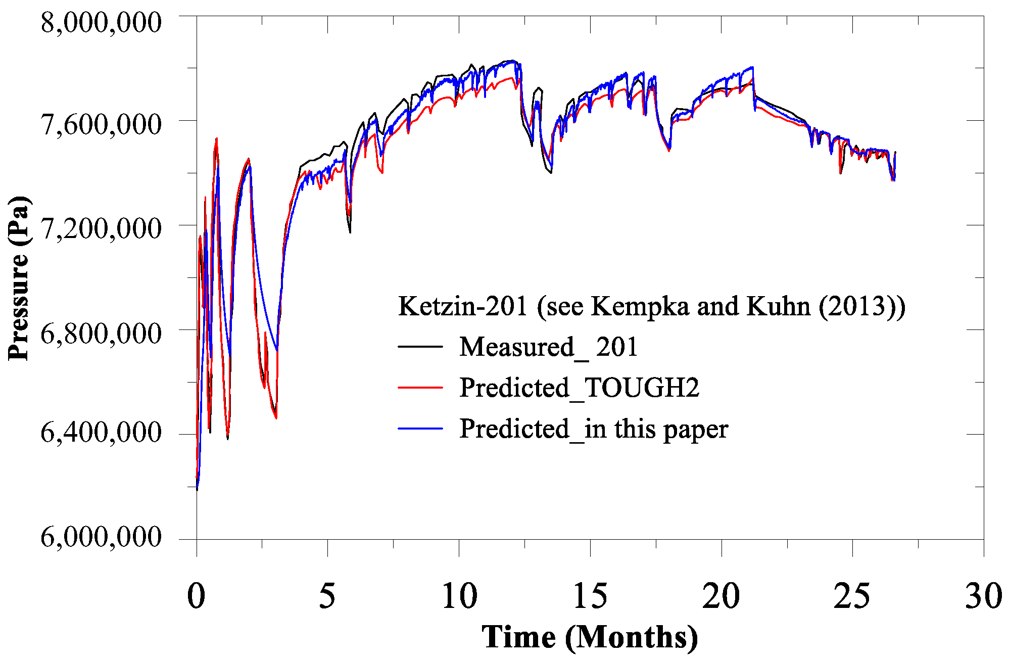
From Kempka and Kühn [20], we obtain the initial pressure and the temperature of the domain as 6.2 MPa and 34 °C (=307.15 K); the storage reservoir was initially fully water saturated (i.e., initial CO₂ gas phase saturation was zero). Along the injection boundary line, the CO₂ gas phase saturation was assumed to be 1, while the temperature was 34 °C. Salinity in the aqueous phase is neglected in the model; total porosity of the solid medium (rock) is 0.25; the isotropic permeability is 4.6 × 10⁻¹⁴ m²; the thermal expansion is 1 × 10⁻⁵; the specific heat capacity is 1.2 × 10³ J/kg/K and the thermal conductivity is 2.5 W/m/K. Pressure response to CO₂ injection was predicted for a simulated period of approximately 27 months. For finite element geometry, we consider the well radius is 0.1 m (Chen et al. [39]). For simplicity, we also assumed the axisymmetric condition. We extended the width of the storage reservoir to 1500 m to minimize the boundary effect in fluid pressure calculation. In Figure 2, we compare 27 months of measured data with predicted data, which has a good agreement, testifying to the accuracy of the model prediction.

In the next section, we used the model in this paper to predict CO₂ leakage through the faulted reservoir. The considered geometry is a simplified, hypothetical section. However, to explain the possible fluids flow through the faulted reservoir, we considered a condition approximately representative of the Ketzin field project (based on previously described literature). This example is useful to demonstrate the simulation of coupled fluids flow in a fault to consider the potential fluid migration and pressure response that may result from such a case.

For the Ketzin site, the carbon dioxide (CO₂) is transported to the sequestration project by road transportation. Then, before starting the injection, CO₂ is stored in the transitional storage tank, where approximate temperature and pressure are −18 °C and 2.1 MPa, respectively (see Ketzin project and Martens et al. [38]; Chen et al. [39]). This type of CO₂ is also known as the cryogenic CO₂ (see also Oldenburg [41]).

Initial reservoir conditions and model assumptions in a hypothetical model follow the same assumptions as presented in the Benchmark Validation section above. The rapid change of fluid conditions from −18 °C and 2.1 MPa in tank storage to 34 °C and 6.2 MPa in the geologic storage reservoir would result in a nearly three-fold volumetric increase (Liebscher et al. [40]). Additionally, the initial state of CO₂ in the Ketzin field project is close to the critical point of CO₂ (31 °C and 7.38 MPa). Hence, the possibility of CO₂ phase transition in the injection well and the reservoir is also high. Thereby, for an identical field case with a fault, it is essential to couple fluids flow, thermal flow, the equation of state and thermo-physics in the model formulation to capture fluids leakage through the faulted reservoir. Additionally, we discuss these physics for an arbitrary case in the next section.

5. Fault Leakage Results

We assume that the study domain is located 1000 m below the ground surface to ensure CO₂ is in the supercritical phase (Rutqvist and Tsang [10]). We consider a simplified geometry to reduce the computational time (Figure 3). The model consisted of a stacked system with two aquifers, two caprocks, and an underlying CO₂ storage reservoir. We also assume a pre-existing fault in the geometry with minimal fault displacement (Figure 3). In this paper, we assume no fault propagation or change to fault properties during simulations. To minimize the computational time, we also consider a constant CO₂ injection rate and monitor the porous media for 300 days. Additionally, we investigate three different injection rates effect, the thermal effect and fault aperture effect in three observation points.

We consider the hydrostatic condition with an average pressure gradient of 10,251.145 Pa/m (Ebigbo et al. [42]). Thereby, we also obtain the initial state pressure at the top and the bottom of the study domain. We also introduce such a condition at the left and the right lateral boundary (the Dirichlet boundary condition), which are constant during the simulation. We also accept that the storage reservoir is initially water saturated, and the CO₂ saturation is zero. However, we assume the CO₂ saturation in the injection point is 1. We assume that the Neumann boundary condition at the top and the bottom of the domain by restricting the flow along the boundary. We consider both the isothermal and the non-isothermal conditions. At the CO₂ injection point (Figure 3), the temperature is 307.15 K. We introduce a low-temperature difference between the study domain boundaries to restrict thermal shock. We assume that caprock layers are impermeable (Ebigbo et al. [42]). We consider that the density, the thermal conductivity and the specific heat capacity of the porous medium are 2650 kg/m³, 3.5 W/(m K) and 750 J/(kg K), respectively (see also Class et al. [43]). We also assume that the porosity, permeability, and diffusion coefficient of the porous media are 0.15, 2 × 10⁻¹⁴ m² and 6 × 10⁻⁷ m²/s respectivly (Ebigbo et al. [42]; Class et al. [43]). We consider that the porous domain is homogeneous and isotropic. Additionally, we obtain fluids properties from Appendix A and Appendix B; Figure A1 and Figure A2.

For the fault, we consider 1D line elements with constant fracture aperture $\left(b\right)$ and corresponding intrinsic fault permeability is $k_f=\frac{b^2}{12}$ (Bear and Berkowitz [44]). We also study the sensitivity of fault aperture considering three types of aperture. For all cases, we assumed fault porosity of 100%.

For finite element mesh generation, we used 103 line elements for the fault and 12,560 triangular elements for other sub-domains (see Figure 3). As the injection rate is slow enough to ensure the applicability of the small deformation theory, we considered the first-order finite elements (Zienkiewicz et al. [45]) with a small time increment $\left(\Delta t\right)$ to ensure the quasistatic condition (Bear and Bachmat [14]).

In the next section, we discuss the injection rate effect, thermal effects, and fault aperture effect.

5.1. Effect of Injection Rate

A safe CO₂ injection rate is essential for any storage reservoir to avoid and or minimize fluids leakage. In a faulted storage reservoir, an excessively high CO₂ injection rate may lead to in situ stress changes that can cause fault activation or dilation with associated effective permeability change, seal fracturing/fracture propagation, and potential increase in leakage rate. While the dynamics of coupled fault mechanics and leakage is not explicitly considered in this manuscript, the relationship between injection rate and leakage through a pre-existing fault of constant aperture is simulated to explore the range of potential leakage. Uncertainty in the sensitivity of the model to injection rate is explored using three different CO₂ injection rates: 0.13773 m³/s, 0.27546 m³/s and 0.41319 m³/s. Simulation results are considered at several observation points (Figure 3) where we predict and compare distributions of pressure, CO₂ mole fraction, density, viscosity, specific heat capacity and thermal conductivity. For the sensitivity analyses in this section, we consider fracture aperture is 100 µm; the temperature gradient is 0.02 °C per meter; the longitudinal dispersivity and transverse dispersivity are 5.0 m and 0.5 m, respectively.

In Figure 4a–c, we observe that close to the injection point pressure evolvement is high, and pressure decreases to the far-field observation points. We also notice in observation point 1, after 18 days, pressure starts to fall for all injection rates, while in observation points 2 and 3, with the injection rate increase, pressure decrease rate reduced. It is noteworthy that during the CO₂ injection, the mean effective stress decreases [10]. In the early stage of CO₂ injection, if the buildup pressure exceeds the allowable stress limit of the porous medium, a fracture may propagate along the compromised faulted reservoir [46]. Moreover, the ratio of the minimum to the maximum injection rate, we assume 3, while we observe that the maximum pressure build-up ratios are 1.128, 1.05 and 1.04, for observation points 1, 2 and 3, respectively. Furthermore, for all injection rates, along the observation points 1 and 2, incremental pressure approach to the steady-state condition, while in observation 3, after 300 days such a condition is not yet achieved, which also justifies the CO₂ distribution as we illustrate in Figure 5.

Figure 5 shows the effect of varying CO₂ injection rates on the distribution of CO₂ saturation (fluid phase mole fraction). We observe that with injection rates 0.13773 m³/s, 0.27546 m³/s and 0.41319 m³/s, in the observation point 1, CO₂ reaches full saturation after 231 days, 99 days and 60 days, respectively. CO₂ saturation in the top formation observation point (Figure 3 and Figure 5), ranges from 0.013 and 0.944 for injection rates 0.13773 m³/s and 0.41319 m³/s, after 300 days.

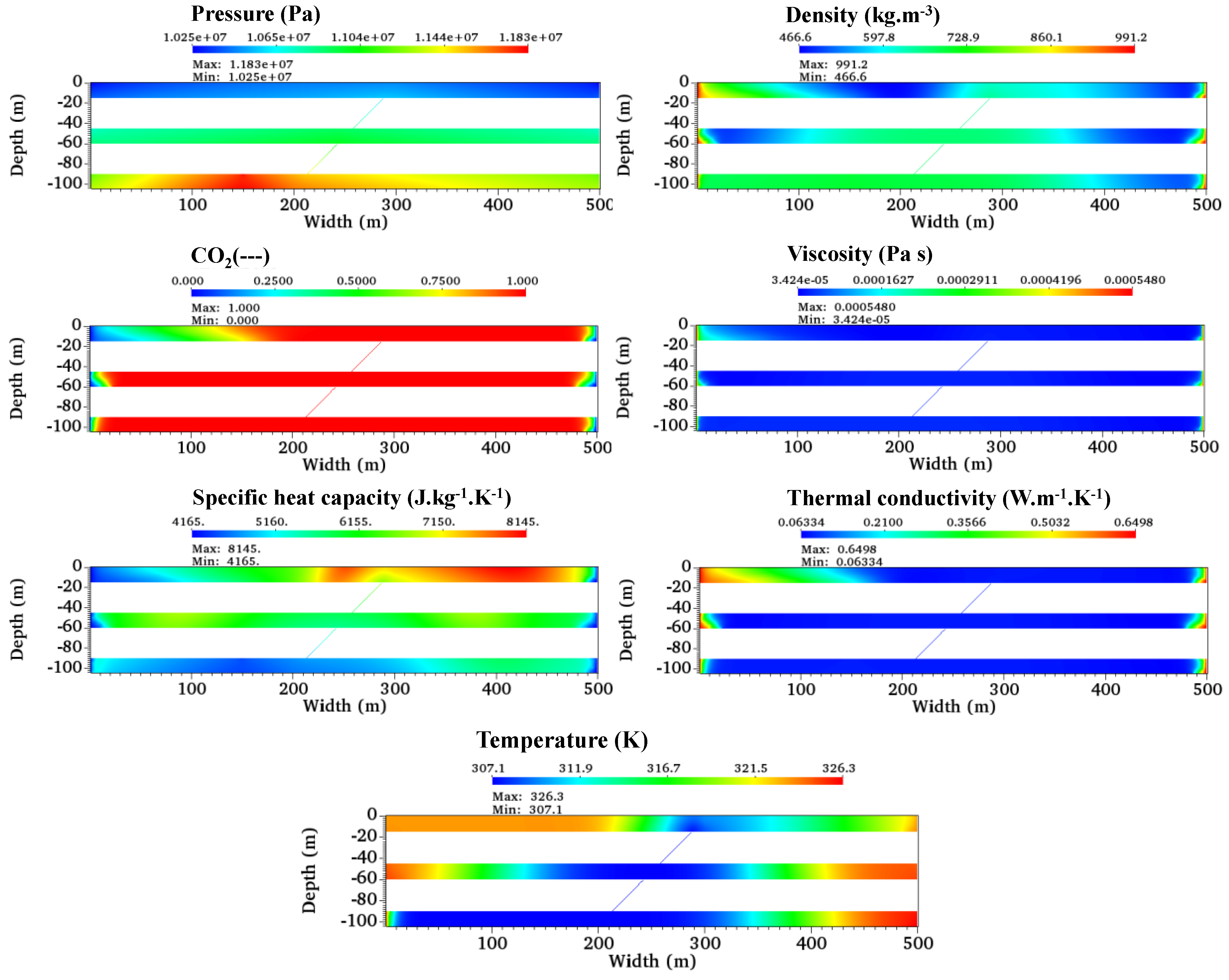
To avoid the repetition of similar illustrations, in Figure 6, we present the spatial distribution of pressure, CO₂ saturation, and fluids properties for the study model domain (Figure 3) after 300 days considering the largest CO₂ injection rate (0.41319 m³/s).

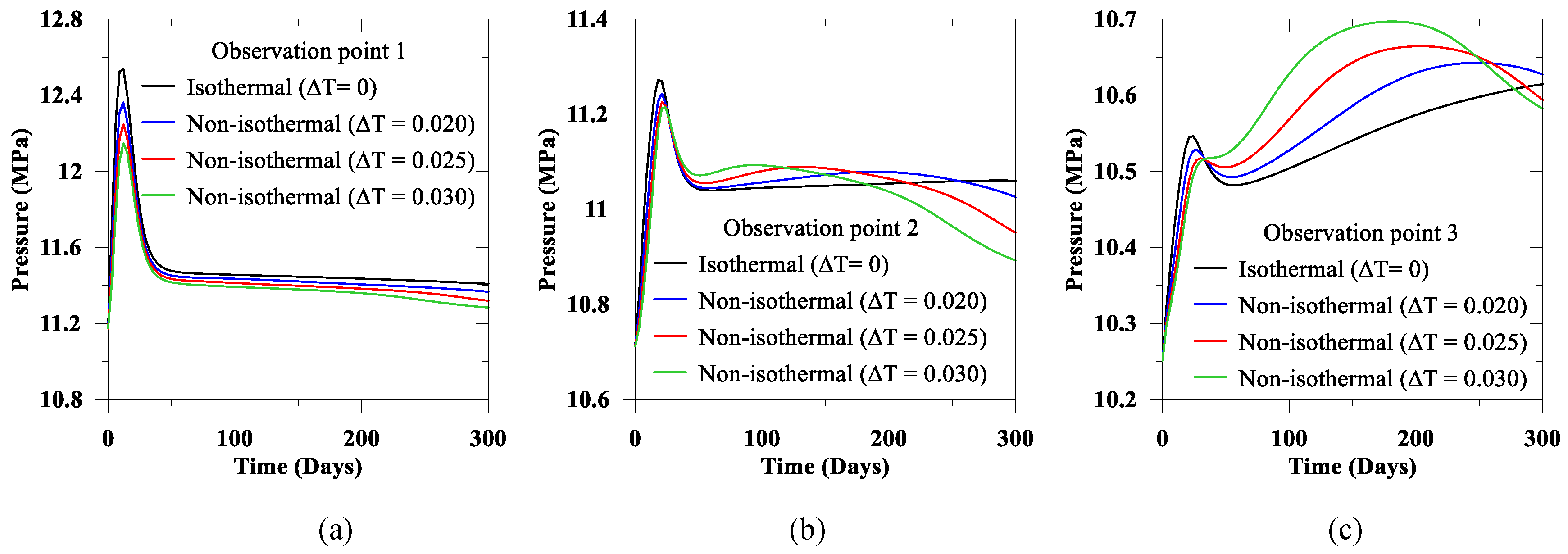
5.2. Thermal Effect

The temperature of CO₂ between the storage reservoir and the transitional storage tank is different. Therefore, it is essential to study the thermal effect of safe reservoir design. Oldenburg [41] also reported that during CO₂ injection, due to the thermal effect, residual fluids in the storage reservoir may freeze and developed thermal stress could generate fracture in the storage reservoir. To explore the potential impact of this phenomenon, we compare injection under both the isothermal and the non-isothermal conditions (considering three thermal gradients: 0.02, 0.025, and 0.030 °C per meter).

Mathias et al. [47] also demonstrated that during injection, CO₂ displaces reservoir fluids causing a gradual pressure increase; as CO₂ expands from the injection point, the reservoir pressure begins to drop. We also observe a similar phenomenon in simulations herein. Figure 7 illustrates the thermal effect on the pressure distribution close to the injection point and the far-field observation points. We find that with the increase of temperature in the near field, there is a decrease in pressure. However, over time, a decrease in temperature and the corresponding increase in pressure is observed in the far-field. We also notice that the temperature gradient effect is significant in the CO₂ mole fraction distribution, and with the increase of the thermal gradient, the CO₂ mole fraction also increases (see Figure 8).

We also present the effect temperature distribution in Figure 9 and Figure 10 for the highest thermal gradient $\Delta T=0.03$ °C per meter, and the isothermal condition. We find that the temperature starts to drop for the non-isothermal state near the injection point. Comparing Figure 9 and Figure 10, we find that the distribution of fluids properties (e.g., density, viscosity) is influenced by the thermal gradient. Additionally, the maximum developed pressure and density in the isothermal condition are higher than in the non-isothermal condition.

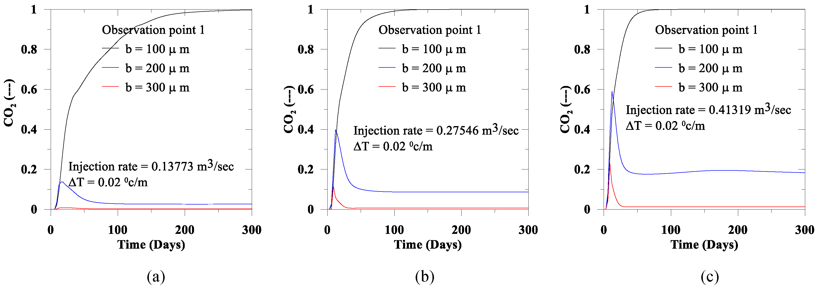
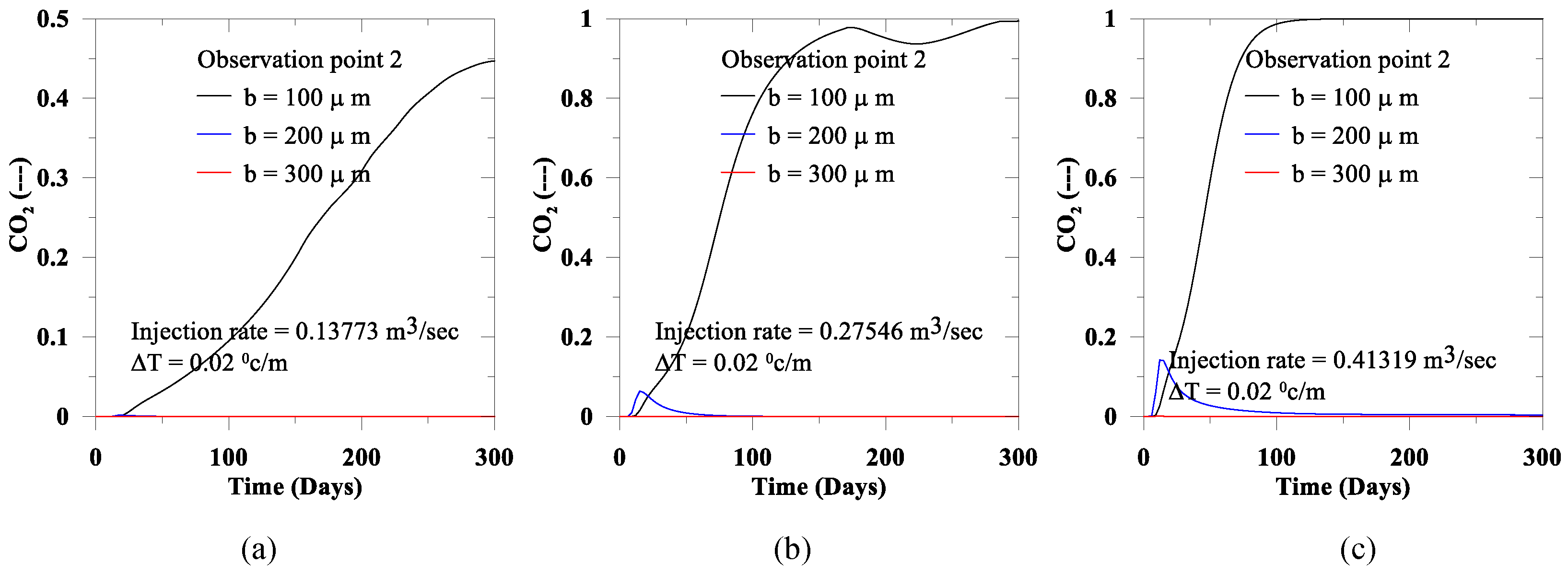
5.3. Effect of Fracture Aperture Size

During and after CO₂ injection, the fracture aperture is playing an important role in the fluid flow pathways. Therefore, in this section, we present the fracture aperture size effect in the near-field and the far-field through three observation points. We consider three different fracture apertures (100 µm, 200 µm, and 300 µm) and injection rates of 0.13773 m³/s, 0.27546 m³/s and 0.41319 m³/s. In the earlier section, we presented the thermal effect, considering the isothermal and the non-isothermal conditions. Therefore, herein we only consider the thermal gradient of 0.02 °C per meter.

In Figure 11, Figure 12 and Figure 13 for all observation points we present the pressure distribution effect on the injection rate and the fracture aperture size. We observe that for observation point 1 (near field to the CO₂ injection) for relatively smaller aperture, the pressure is relatively high compared to the increase of fault aperture. In this paper, as we consider the fracture aperture is constant throughout the simulation; therefore, with the increase of aperture, the path to fluid flow experienced less resistance than a small conduit aperture. As a result, in the near field, the developed pressure for any specific thermal gradient is inversely proportional to the fault aperture. In contrast, for an identical thermal gradient and the near field condition, the developed pressure is proportional to the CO₂ injection rate. However, in the relatively far field (e.g., Observation points 2 and 3), due to the energy dissipation during flow path in the space, the observed response for the pressure is opposite to the near field condition. Therefore, close to the injection point, the presence of fracture requires additional attention to avoid the instabilities due to the developed pressure in the near field.

In Figure 14, Figure 15, Figure 16 and Figure 17, we present CO₂ distribution at three observation points. The CO₂ leakage through the larger aperture is high compared to the small aperture. Therefore, we observe that in all observation points, the CO₂ presence is inversely proportional to the aperture size. In contrast, CO₂ distribution increase with the increase of the injection rate and the thermal gradient.

6. Conclusions

In this paper, we present a coupled finite element solution combining the mass balance equations of fluids phase, the energy balance equations, and the fractional mass transport equation. For the solution of pressure and temperature variables, we consider the monolithic coupling, while for the mass transport, we used the staggered approach [48]. Additionally, to obtain the thermo-physical fluids properties, we also use the Peng-Robinson Equation of State (EoS). For the validation of solution algorithms, we compare coupled finite element (FE) results with the Ketzin pilot project measured responses for 27 months and with the TOUGH predicted results, which show a good agreement and testify the performance of FE results.

We also present fluids flow through a faulted reservoir, demonstrating the effect of the CO₂ injection rate, the thermal effect, and the fault aperture effect. We observe that during injection, the buildup of pressure and its distribution, the thermal gradients also change the thermo-physical fluids properties. Moreover, close to the injection point’s low temperature compared to the domain also reduce the temperature along the fluids flow path, which also justifies the importance of the thermal effect in the CO₂ sequestration project. Herein, to avoid thermal shocks, we consider a low temperature gradient. However, if the temperature drop is too high, it may adversely impact the CO₂ injection.

We observe that during CO₂ injection, for a specific thermal gradient, the developed pressure and CO₂ concentration is proportional to the injection rate. Again, for the non-isothermal condition, the developed pressure in the near field is high compared to the far field condition. In contrast, in the far field, the pressure is proportional to the thermal gradient, and the magnitude is lowest for the isothermal condition. We also observed that CO₂ concentration for all observation points is proportional to the thermal gradient. For a specific injection rate, the density, the viscosity, and the thermal conductivity decrease with the thermal gradient increase. However, the specific heat capacity increase with the increase of the thermal gradient. Additionally, in the near field, for a particular thermal gradient and an injection rate, the developed pressure is inversely proportional to the fracture aperture. In contrast, for the far field, we noticed the opposite behavior. For all observation points, CO₂ concentration is inversely proportional to the fracture aperture.

For the faulted reservoir, the safe injection rate is crucial to avoid the instabilities of the storage reservoir. In such a condition, developed pressure and CO₂ saturation are both crucial. The temperature of CO₂ in the transitional storage tank is relatively low compared to the storage reservoir. Therefore, it is essential to assess the effect of injection rate, temperature, and the aperture of fault in the near field and the far field condition to limit the CO₂ leakage, which we addressed through a hypothetical faulted reservoir.