An Introduction to the Geometrical Stability Index: A Fabric Quantity

Abstract

Natural soils are often modelled as a continuum characterized by the composition of the soil, a particulate material. Yet, in situ, the fabric and structure of soil may govern its behavior. Discrete element modelling is used to simulate the composition of soil as a particulate material and develop fabric quantities. These quantities are presented as average quantities for a volume of particles. It is possible to use DEM to study the evolution of fabric at the particle level. This paper describes a state-of-the-art fabric term, referred to as geometrical stability index, $ʎ$, which can measure the contacts deviation of each particle from the most stable contacts arrangement during loading. The parameters required to define this new fabric term were attained from a designed algorithm. 2D discrete element method (DEM) biaxial test simulations were performed to validate the effectiveness of the geometrical stability index in defining the local instability. As the sample is loaded, a shear band is formed. The geometric stability index in that band increases relative to the surrounding relatively intact soil. Thus, a brittle failure is associated with an increase in the variation of inter-particle contacts from a stable configuration. The geometric stability index is able to model the development of discontinuities in a particulate material at the particle level. The DEM modelling results demonstrate the correlations between the new fabric term and the progressive of localized failure in densified particulate systems such as over consolidated clay, where the failure is a function of progressive development of local fissure spacing.

1. Introduction

Experimental and theoretical soil mechanics are often based on the concept that soil is a continuum and can exhibit in two states depending on the composition, yet fabric and structure can be the dominant factors controlling the behavior. For example, the strength of clays, especially over consolidated clays, is a function of fissure spacing; failure mechanisms in slopes depend on fissures, faults, and bedding planes. These features, that is fissures, fractures, and other discontinuities, cannot easily be addressed in continuum mechanics therefore some correction factor is applied. For example, the strength of a fissured soil may be reduced by 50%. This addresses a possible strength reduction but does not address the alignment of the fabric features which can be critical in stability analyses.

Granular materials are made up of discrete particles in contact. A drift in displacement of any particle having one or more contacts about its equilibrium position during loading results in changing in contact networks of particles. These alterations may lead to lost contacts or new contacts between particles. The static and dynamic behavior of such granular material is influenced by these alterations (i.e., fabric evolution). Studying the fabric evolution of granular materials during loading opens a new window to advance our understanding on the responses of such materials. The early works related to the study of particulate systems fabric can be found in [1,2,3,4,5]. In these works, the fabric evolution, and its effect on the macro-mechanical behavior of sand subjected to static load were experimentally studied. Monitoring the evolution of contact configuration at different stages of loading process is, however, difficult to observe. Optical technology such as X-ray diffraction and electronic measurement techniques was used by a number of researchers (e.g., [6,7]) to study the evolution of granular materials for quantitative and qualitative studies. However, analyzing the fabric and its effect on the macro-micro mechanical behavior by means of experimental tests or analytical methods is still considered difficult (e.g., [8]). Alternatively, DEM based simulations, which was pioneered by [9], can provide the particle-level information of idealized granular system such as particle movements and rotations. This method was proved a strong tool to study fabric evolution of granular systems under loading [8,9,10,11,12,13,14,15,16]. One of the key fabric quantities is average coordination number. This parameter is the average number of contacts per particle within a specific volume of a particulate assembly and consequently it provides a measure of packing density or packing intensity of fabric at particle-level. However, this average fabric quantity cannot show how contacts are distributed around a particle. This issue was considered in average normal contact distribution which is a tensor quantity and statistically describes the orientation of contacts during loading. These fabric terms, which are collective terms, can be used to interpret the bulk stability of granular system and give an indication of the response and bulk instability since the stability of such granular material is influenced by contact arrangement of each particle [17,18]. However, instability can occur at a particle level which may progress causing local instability.

The fabric of a soil, which is the size, shape and arrangement of soil particles, influence macro behavior. Constitutive models developed for fine and coarse grain6ed soils can take account of particle size and density by changing the hydraulic, stiffness and strength characteristics. It is assumed that these characteristics are a function of particle size and soil density, but they are not intrinsic properties as they are affected by the mean stress and soil fabric. This behavior can be modelled with an appropriate constitutive model. However, it is more difficult to model the influence of fabric on soil structure yet understanding the effect of micromechanical behavior on mechanical response is necessary. For example, the progressive development of slip surfaces would allow potential failure mechanisms to be anticipated. Discrete element methods allow this micro behavior to be studied. This paper focuses on the fabric of soil and how it leads to instability with the introduction of a new factor, the geometrical stability index. The new concept was then validated by DEM modeling.

2. DEM Implementation in PFC^2D

DEM Contact Kinetics

In this paper, the simulations are conducted with commercial software PFC^2D 4.1 [19]. The rolling resistance is not adopted in the presented simulations. O’Sullivan et al. [20] experimentally showed that if the particle size is larger than 0.1 mm, the surface roughness will have a minor impact on the material behavior in comparison with the particle inertia. The PFC^2D code considers the tangential component of the contact force. The contact force (${\mathit{F}}_{\mathit{i}}$) applied on a disk particle is decomposed into tangential force (${\mathit{F}}_{\mathit{i}}^{\mathit{s}}$) and normal force (${\mathit{F}}_{\mathit{i}}^{\mathit{n}}$). The former is directed along the tangent to the particle and the latter is directed toward the particle center.

$${\mathit{F}}_{\mathit{i}}={\mathit{F}}_{\mathit{i}}^{\mathit{n}}+{\mathit{F}}_{\mathit{i}}^{\mathit{s}}$$

(1)

In PFC^2D, it is assumed that disks are rigid with soft contact. That is, a contact overlap between two particles (e.g., a and b) is applied rather than a contact deformation. The magnitude of this overlap is computed by contact law. The linear elastic contact law is used to calculate the normal and tangential contact forces in this study. The normal and tangential displacements at time step ${\Delta }_{\mathbf{t}}$ is calculated as follows:

$${\Delta }_{\mathit{n}}=\left[\left({\dot{\mathbf{x}}}^{\mathit{b}}-{\dot{\mathbf{x}}}^{\mathit{a}}\right)\right] \mathit{n} {\Delta }_{\mathbf{t}}$$

(2)

$${\Delta }_{\mathit{s}}=\left\{\left[\left({\dot{\mathbf{x}}}^{\mathit{b}}-{\dot{\mathbf{x}}}^{\mathit{a}}\right)\right]\mathit{t}-\left({\dot{\mathit{\theta }}}^{\mathit{a}}\left|{\mathit{R}}^{\mathit{a}}\right|+{\dot{\mathit{\theta }}}^{\mathit{b}}{\mathit{R}}^{\mathit{b}}\right)\right\}{\Delta }_{\mathit{t}}$$

where ${\dot{\mathbf{x}}}^{\mathit{a}}$, ${\dot{\mathbf{x}}}^{\mathit{b}}$, ${\dot{\mathit{\theta }}}^{\mathit{a}}$ and ${\dot{\mathit{\theta }}}^{\mathit{b}}$ are translational and rotational particle velocities of particle a and b, respectively. ${\mathit{R}}^{\mathit{a}}$ and ${\mathit{R}}^{\mathit{b}}$ are the particle radius. $\mathit{n}$ and $\mathit{t}$ are the normal and tangential unit vector of.

The magnitude of the normal and tangential contact forces is calculated via:

$${\left({\mathit{F}}_{\mathit{i}}^{\mathit{n}}\right)}_{\mathit{t}}= {\left({\mathit{F}}_{\mathit{i}}^{\mathit{n}}\right)}_{\mathit{t}-\mathbf{1}}+{\left(\Delta {\mathit{F}}_{\mathit{t}}^{\mathit{n}}\right)}_{\mathit{t}}$$

(3)

where $\Delta {\mathit{F}}_{\mathit{t}}^{\mathit{n}}={\mathit{K}}_{\mathit{n}}{\left({\Delta }_{\mathit{n}}\right)}_{\mathit{t}}$

$${\left({\mathit{F}}_{\mathit{i}}^{\mathit{s}}\right)}_{\mathit{t}}= {\left({\mathit{F}}_{\mathit{i}}^{\mathit{s}}\right)}_{\mathit{t}-\mathbf{1}}+{\left(\Delta {\mathit{F}}_{\mathit{t}}^{\mathit{s}}\right)}_{\mathit{t}}<\mu {\left({\mathit{F}}_{\mathit{i}}^{\mathit{n}}\right)}_{\mathit{t}}$$

(4)

where $\Delta {\mathit{F}}_{\mathit{t}}^{\mathit{s}}={\mathit{K}}_{\mathit{s}}{\left({\Delta }_{\mathit{s}}\right)}_{\mathit{t}}$

The total contact shear force is compared to the Coulomb sliding friction criterion to check whether the sliding has occurred. When the resultant force and torque in the z-direction (calculated by multiplying tangential contact force by the distance from the particle center to the contact location) are computed for each particle, the local damping force ${\mathit{F}}_{\mathit{i}}^{\mathit{d}}$ will be added to them:

$$\mathit{F}={{\displaystyle \sum }}^{ }[{\left({\mathit{F}}_{\mathit{i}}^{\mathit{n}}\right)}_{\mathbf{t}}\mathit{n}+{\left({\mathit{F}}_{\mathit{i}}^{\mathit{s}}\right)}_{\mathbf{t}}\mathit{t}]+{\mathit{F}}_{\mathit{i}}^{\mathit{d}}$$

$$\mathit{M}=[\mathbf{R}{{\displaystyle \sum }}^{ }[{\left({\mathit{F}}_{\mathit{i}}^{\mathit{s}}\right)}_{\mathbf{t}}\mathit{t}]+{\mathit{F}}_{\mathit{i}}^{\mathit{d}}$$

(5)

$${\mathit{F}}_{\mathit{i}}^{\mathit{d}}=-\mathit{\alpha }\left|\mathit{F}\right|\mathit{s}\mathit{i}\mathit{g}\mathit{n}\left(\dot{\mathit{x}}\right); \mathit{s}\mathit{i}\mathit{g}\mathit{n}\left(\dot{\mathit{x}}\right)=\{\begin{array}{c}+\mathbf{1}, \mathsf{i}\mathsf{f} \dot{\mathit{x}}>\mathbf{0} \\ -\mathbf{1}, \mathsf{i}\mathsf{f} \dot{\mathit{x}}<\mathbf{0} \\ \mathbf{0}, \mathsf{i}\mathsf{f} \dot{\mathit{x}}=\mathbf{0} \end{array}$$

where $\mathit{\alpha }$, $\left|\mathit{F}\right|$ and $\dot{\mathbf{x}}$ are damping constant, resultant force on the particle and particle velocity, respectively. The computed resultant force and torque acting on the particle is used to determine the change in particle velocity via Newton’s second law for the next time step.

3. Soil Fabric

In geological terms, soil fabric is the size, shape and arrangement of soil particles, a similar definition to that used in granular mechanics. Fabric quantities include the coordination number which increases with densification [18] particle orientation if noncircular particles are used, contact orientation and branch vector orientation for non-circular particles. These factors are often presented as an average (e.g., change in coordination number with macro displacement) or graphically (e.g., polar diagram of contacts). Kruyt and Rothenburg [21] and Potyondy and Cundall [22] discusses means of using a DEM to relate the macro performance and the interaction between particles including the force chain network, particle displacements and rotations. DEM allows detailed study of zones within the model using reference volumes, mechanical coordination number. Rothenburg and Bathurst, 1989 [17] proposed a closed form solution to estimate the polar diagram of contacts.

$$E\left(\theta \right)=\frac{1}{2\pi }\left[1+a\cos 2\left(\theta -{\theta }_a\right)\right]$$

(6)

where $a$ represents “fabric anisotropy” in a granular system, depending on the number and density of unit normal vectors in principles axes. In fact, $E\left(\theta \right)$ shows the deviation between the geometry of contact force distribution and the isotropic geometrical contact force distribution. For example, if $a=0$, $E\left(\theta \right)$ will be a circle such that the state of the system being considered is in an isotropic state. ${\theta }_a \mathrm{is}$ the direction of anisotropy. Parameters, $a \mathrm{and} {\theta }_a$, are obtained by the following equations:

$$a=\frac{2\sin \Delta \theta }{N\Delta \theta }\sqrt{[{\displaystyle \sum }_{g=1}^{n_g}{N}_g\sin {\left(\left(2g-1\right)\Delta \theta \right]}^2+[{\displaystyle \sum }_{g=1}^{n_g}{N}_g\cos {\left(\left(2g-1\right)\Delta \theta \right]}^2}$$

(7)

$${\theta }_a=\frac{1}{2}{\tan }^{-1}\frac{{\sum }_{g=1}^{n_g}{N}_g\sin (\left(2g-1\right)\Delta \theta }{{\sum }_{g=1}^{n_g}{N}_g\cos (\left(2g-1\right)\Delta \theta }$$

(8)

where $N$ is the total number of contact, $\Delta \theta =\frac{360}{n_g}$, $n_g$ the number of segments and $N_g$ is the number of contacts within the $g$^th segment. In fact, these fabric anisotropy parameters show the ability of granular systems to create the anisotropy state in normal contact distribution.

These statistical methods provide an insight into material behavior relating the macro behavior to the mechanism at particle level. Hall et al. [23] used X-ray micro tomography imaging with 3D volumetric digital image correlation techniques to study the kinematic development of shear bands within a triaxial compression test to show that a narrow shear band post peak stress starts with the development of strain across a broad zone of soil.

The development of a shear surface within a dense granular material is associated with a reduction in particle contacts since the density of the shear zone is less than the density of the surrounding soil. Therefore, it is necessary to study the local displacements rather than the average response. Further, the reduction in particle contacts is also associated with an alignment of the contacts.

4. Fabric Development

A load difference applied to a particulate system creates a bias in the orientation of contact networks and chain forces to generate a major load path at its maximum capacity [24]). This re-arrangement of contacts leads to “fabric anisotropy” in a granular system. The maximum soil strength is, therefore, coincidence with the peak of fabric anisotropy since the number of contacts in the direction of the major principal stress axis is higher than those in the direction of the minor axis. The increase in average fabric anisotropy is associated with an increase in bulk instability but it is also associated with local instability demonstrated by the formation of a shear band. Conversely, if a discontinuity exists then this could reduce the capacity of the system as it may become the preferred zone of weakness. Thus, the average coordination number and fabric anisotropy could not represent the fabric properties within the failure zone even though the fabric in that zone governs the failure. Therefore, a new term is required to count for the discontinuity.

A particle is stable if equally spaced contact forces are equal. If there is any change in the contact distribution, there must be a change in the contact forces to maintain stability. This does not mean a particle becomes more unstable; it does mean that there is an increase in the major contact force and an increase in the force difference. Particle movement to ensure local stability could accompany this process. As the variation between the uniform distribution of contact forces and the current distribution increases, fabric will develop as particles move to maintain equilibrium, eventually leading to a shear zone. An equal distribution of contacts of a particle is defined as the most stable contact distribution and the deviation of the contact distribution from the most stable contact distribution is the geometric stability index, a fabric quantity.

5. The Stability Index

Assume a particle is in contact with n particles, then a set of n-stable contact arrangements, $S^n$ is defined. The radial distance between two contacts on the perimeter of a particle is defined as the minimum angle between them. The deviation of the contact arrangement, $d^{Sn}$, from a stable configuration is expressed as the sum of the deviation of each contact point from the associated stable location starting with the first contact point such that:

$$d^{Sn}={\displaystyle \sum }_{i=1}^{n}d\left(S_i^n\right)$$

(9)

This is repeated for each contact point; that is, the sum of the variation on n contact points is calculated n times. Thus, for n contacts there are n possible variations from the stable configuration. The minimum value of $d^{Sn}$ is D, such that:

$$D=\min \left\{d^{Sn}\right\}$$

(10)

in which D is the minimum radial distance for a particle with n contacts from the stable contact arrangement. To make it dimensionless, it is divided by 360°.

$$\lambda =\frac{D_M}{360}$$

(11)

in which $\lambda$ is stability index. The algorithm was provided to determine this term was schematically shown as flowchart in Figure 1. In the first step, a loop is executed upon all particles to find a particle. A search around this particle is then carried out to find its active contacts. The angles between these contacts are then calculated and stored into an array. Particles with one or no contact are not stable and are assigned a value of λ of one. It is since this particle cannot contribute to force transfer and it is not also stable. λ for a geometrically stable configuration is zero which only applies to particles with two or more contacts. Particles with two contacts can be stable provided the contact points are diametrically opposite. If the particle is in contact with more than three particles, the current contact arrangement will be compared with the corresponding n-stable contacts arrangements to calculate the n radial distances (i.e., ${\lambda }_1,$ ${\lambda }_2,{\lambda }_3$, …, ${\lambda }_n$). The geometrical stability index for this particle the is calculated as $\lambda =$ Min (${\lambda }_1,$ ${\lambda }_2,{\lambda }_3$, …, ${\lambda }_n$). Next this particle will be marked and stored into an array. This cycle will be continued for all particles in the system.

For example, consider (Figure 2) three particles, A, B and C, in contact with a fourth particle, D, such that, relative to the line joining the centers of A and D, a set of 3-stable contact arrangements can be defined for this current contact configuration (i.e., Sⁿ = S³). Figure 3a–c shows three stable contact arrangements. If the angle between particle A and particle B is 120° and the angle between particle B and particle C is 120°, there is geometric stability. If either of these angles ≠ 120° then the configuration is no longer geometrically stable. This can be expressed in terms of the deviation of the lines connecting the centers of the particles from the geometrically stable configuration. The dash lines in each of these figures is the stable contact configuration. The angle between them is 120°.

The sum of the variation from the stable configuration is calculated for each contact point; that is for three contacts, there are three values of d^Sn and for each contact point, d^Sn is the sum of two angles since the variation from the stable configuration for one contact must be zero. For the first set (Figure 3a):

$$d^{S{n}^A}={\alpha }_1+{\alpha }_2$$

(12)

For the second set (Figure 3b)

$$d^{S{n}^B}={\beta }_1+{\beta }_2$$

(13)

For the third set (Figure 3c):

$$d^{S{n}^C}={\gamma }_1+{\gamma }_2$$

(14)

Thus, the geometric stability index for this particle is:

$${\lambda }_2=\frac{min \{d^{S{n}^A}, d^{S{n}^B}, d^{S{n}^C}\}}{360}$$

(15)

Note that particle size is not considered in this analysis. For example, if particles D, A and B are of equal size then α_B cannot be less than 30° since at that point the particles A and B are in contact.

For an equal distribution of contact points, the geometric stability index for an isotopically stable arrangement is zero. At that point the contact forces are equal. In practice, λ will be greater than zero since a sample is a random packing of particles of various sizes. As the difference in contact forces increases the arrangement of the contact forces will change which means the λ must increase in order to maintain equilibrium. The maximum value of λ depends on the particle dimensions but for four equal diameter particles (that is three contacts) λ_max is 0.333.

6. Fabric Evolution

Fabric evolution was studied in a 2D biaxial test modelled with PFC^2D, discrete element modelling software [19]. The sample tested was formed of particles varying from 0.5 mm to 3 mm in diameter corresponding to a well graded sand shown in Figure 3. These were randomly placed within a biaxial chamber with rigid walls. The diameters of the particles were halved and then expanded randomly until a target porosity of 0.12 was achieved. The time step required to simulate the biaxial test has to be very small in order to prevent instability of the model. If it is a quasi-static simulation, it is possible to increase the time step by scaling the density. The density scaling factor, $I$, in the following equation must be less than 10⁻³ [25].

$$I=\sqrt{\frac{{\dot{\epsilon }}^2\rho r_{min}^2}{p_y}}$$

(16)

where $\dot{\epsilon }$, $r_{min}$, $p_y$ and $\rho$ are the strain rate, the minimum radius of the particles, the limiting contact pressure between particles and the density of the particles. There is a transition zone in the behavior of the materials near $I$ = 10⁻³ for which higher values of $I$ leads to a transient and dynamic behavior, and the behavior maintains a quasi-static response for lower values. The final particle size distribution is displaced in Figure 4.

Table 1. The initial porosity and micro-mechanical properties of the sample.

Initial Porosity	0.12
Range of PSD [mm]	0.5–3
$K_n\left(\frac{N}{m}\right)$ [Normal contact stiffness]	8.45 × 107
$K_s \left(\frac{N}{m}\right)$ [Shear contact stiffness]	8.45 × 107
μ [Coefficient friction of particle]	0.9
α [Damping constant]	0.8
Coefficient friction of particle-platen	0.0
Width [mm]	75
Height [mm]	150
$\dot{\epsilon }$	$\frac{2\%}{\min }$
$\rho$$(\frac{\mathrm{kg}}{{\mathrm{m}}^3}$)	2 × 108
$R_{min}$$(\mathrm{mm}$)	0.236
$p_y$(MPa)	150

shows the input data used for this test. Next, the sample was isotopically consolidated to 100 [kPa]. Additional cycles then executed to bring the system to the static equilibrium. The rigid walls were replaced by deformable boundary [26] represented by particles at the edges of the sample which formed continuous boundaries to the sample (see Figure 5). The top and bottom platens are then moved slowly inward at a constant velocity to perform a biaxial test. The strain rate applied for this test was $\frac{2\%}{\min }$ such that the incremental acceleration of each particle at each time step is small. A sensitivity analysis showed that the particle density $\rho$ = 2 × 10⁸ $(\frac{\mathrm{kg}}{{\mathrm{m}}^3}$) can reproduce the similar macro-micro behavior as real particle density $\rho$ = 2650 $(\frac{\mathrm{kg}}{{\mathrm{m}}^3}$).

The polar diagrams of normal contact distribution and normal contact force distribution at isotropic consolidation are shown in Figure 6 and Figure 7. To draw these polar diagram 18 bins were considered with an angular interval $\mathsf{\Delta }\theta$ = 20°. The radius of each bin in the polar diagram of normal contact and normal contact force distribution corresponds to the number of contacts and summation of normal contact forces within each angular interval. If polar diagram of is fully circle, it shows that the distribution of normal contact and normal contact force is in isotropic state. That is $a$ and $a_n$ = 0. Although the sample is in isotropic state at macro-scale, it can be seen from Figure 6 and Figure 7 that there is anisotropy in fabric of contacts and normal contact forces at this stage, $a$ = 0.0034 and $a_n$ = 0.009.

The details of $E\left(\theta \right)$ have been explained from Equations (6)–(8). $F_n\left(\theta \right)$ mentioned in Figure 7 shows the deviation between the geometry of normal contact force distribution and the isotropic geometrical normal contact force distribution of a granular system [17]. The variation of stress ratio with axial strain is shown in Figure 8. The macro stress-strain behavior until ${\epsilon }_{11}$ = 0.5% seems to be linear elastic. From ${\epsilon }_{11}$ = 0.5% to ${\epsilon }_{11}$ = 1.5% the soil shows a hardening-strain behavior, characterizing either dense sand or over-consolidated clay [27]. From ${\epsilon }_{11}$ = 1.5% onward the critical state behavior.

The microscopic behavior of the sample being considered is shown in Figure 9 and Figure 10. In spite of showing a linear trend until ${\epsilon }_{11}$ = 0.5% in Figure 8, changes at the microscopic level are not a reversal. It is due to permanent change in the fabric of a particulate system such that the fabric anisotropy increases rapidly from 0.0034 at ${\epsilon }_{11}$ = 0% (i.e., isotropic state) to around 0.18 at ${\epsilon }_{11}$ = 0.5%. The axial strain corresponding to maximum fabric anisotropy is almost similar with peak stress-strain in Figure 8. From ${\epsilon }_{11}$ = 0% to ${\epsilon }_{11}$ = 0.15% the particulate system can be significantly changed in its contact arrangements to show the maximum strength. After reaching the peak, the trend of fabric anisotropy significantly decreases and reach toa constant value, suggesting the critical state behavior.

Figure 10 shows the variation of average coordination number with axial strain. As seen the average of contacts per particle decrease considerably from around 3.9 at ${\epsilon }_{11}$ = 0% to around 3.0 at ${\epsilon }_{11}$ = 0.15%, corresponding the peak strength of system. This shows that the soil behavior is non-linear elastic since the particulate system lost their contacts significantly even at lower stress level. From ${\epsilon }_{11}$ = 0.15% onward the average coordination number becomes constant. Considering the microscopic behaviors (Figure 9 and Figure 10) makes this argument clear that the bulk instability is coincidence with peak fabric anisotropy and inflection point in average coordination number with axial.

By increasing the vertical load while the stress at the side boundaries kept constant through the stress control, the particulate system is sheared. The progress of shear plane development during loading is seen in Figure 11 in which the legend shows the particle displacements varying from 0 [m] to 10⁻³ [m]. Notedly, only the scaler field of displacements is considered here. The cumulative particle displacements at an axial strain of 0.5% is shown in Figure 11a. As the rigid platens move together the sample develops a diagonal zone in which the particle displacements are less than the rest of sample. The magnitude of particles displacements decreases gradually from end restraints to the diagonal zone. The reduction in particle displacement is accompanied by lateral expansion of the sample. As the stress ratio increases, the particle displacements increase (in the lighter zones) and the width of the diagonal zone reduces (Figure 11b) leading to the development of the shear plane at an axial strain of 0.9% (Figure 11c). The shear plane is fully developed (Figure 11d) at an axial strain of 1.5%, which corresponds to the peak stress ratio. Figure 11e shows the cumulative particle displacements at the end of the simulation. This figure shows that an increase in axial strain after the peak stress does not have a significant effect on the displacement field within the shear zone. (Cheung and O’Sullivan, 2008) [28] and (Wu et al., 2020) [29] showed that the rotation of the particles within the shear band is significantly larger than the rest of the sample. Therefore, particle rotation within the shear plane dominates the behavior rather than particle displacement; that is turbulent shear rather than sliding shear dominates. Very few microscale tests on shear band evolution could be found in the literature. Tomographic technique was used to study the shear band formation during triaxial tests. However, this technique is costly and experimental results were scarcely available and very sensitive to the testing conditions, hence difficult to be used to validate the outcomes from this research. For qualitative validation, image from bulk level test showing the shear band formation is used to compare with the present study as appeared in Figure 11f [30]. It can be observed that similar pattern of shear band formation and failure plane can be observed by comparing Figure 11e,f.

Alternatively, computational methods are often used to study the shear band development of soil during shearing. (Medicus and Schneider-Muntau, 2019) [31] conducted a numerical study using the finite element method on fine material to investigate the evolution of shear band during the biaxial test. They found that the shear bands commence from the beginning of the test, and it develops well before the peak stress (see Figure 11g). Their observations on shear band formation qualitatively in good agreement with the present research.

Figure 12 shows the development of the fabric expressed in terms of geometrical stability index at axial strain of 0.5%, 0.7%, 0.9%, 1.5%, and 10%. The sample starts with randomly distributed stability indices suggesting that this is a uniform sample with no discontinuities (Figure 12a). At 0.5% strain there is evidence (Figure 12b) of the development of a discontinuity surrounded by more stable particles. Further strain increase leads to a more clearly defined shear zone (represented by particles with a stability index exceeding 0. 5). It also shows that the remainder of the sample also becomes less stable with evidence of shear taking place throughout the sample parallel to the clearly defined shear zone. These modelling results clearly demonstrated the correlations between the newly developed Geometrical stability index and the macro behavior of the particle system, such as the development of shear band. In the research carried out by (Medicus and Schneider-Muntau, 2019) [31], they observed the shear strain is higher at the shear band in comparison with the rest of the model (see Figure 11g), meaning the particles have less support at this zone (e.g., contacts). This fact has been observed in Figure 12, showing particles are less stable at the shear band and consequently cannot contribute to force transition across the model.

Figure 13a shows that the majority of those particles are in shear band have two contacts at ${\epsilon }_{11}$ = 1.5% while the rest of particles have at least three contacts (see Figure 13b). Note, those particles with one and zero contacts were filter out. The average geometric stability index in the shear zone at peak stress ratio is 0.34 and the average in the remainder of the sample 0.31.

The variation of average geometric stability index with axial strain is shown in Figure 14. The trend of this average quantity is in good agreement with the trend of stress ratio and fabric anisotropy with axial strain (Figure 9). The graph also shows that up to peak stress ratio, the geometric stability index increases from its initial stable contact arrangement and then reduces to a constant value post peak. This is consistent with the distribution of the geometric stability indices in Figure 12f which shows a pattern similar to that at peak stress (Figure 12e).

7. Discussion

Figure 12 and Figure 13 suggest that there may be a relationship between the coordination number and λ since the shear zone coincides with minimum coordination number and the maximum λ. Nineteen simulations, including irregular and hexagonal packing, were carried out. The hexagonal arrangement, the most stable arrangement for a granular system, was created using single sized particles. The inter-particle properties, boundary conditions and mean particle size for all of these tests were the same.

Table 2. The micro-mechanical properties of the irregular packing sample.

Initial Porosity	0.08, 0.09, 0.1, 0.11, 0.12, 0.13, 0.14, 0.15, 0.16, 0161, 0.165
Range of PSD [mm]	0.5–3
$K_n$	8.45 × 107
$K_s$	8.45 × 107
μ [Coefficient friction of particle]	0.9
α [Damping constant]	0.8
Coefficient friction of particle-platen	0.0
Width [mm]	75
Height [mm]	150
$\dot{\epsilon }$	$\frac{2\%}{\min }$
$\rho$	2 × 108
Range of particle size	0.25–1.5

and

Table 3. The micro-mechanical properties of the hexagonal packing sample.

Initial Porosity	0.08, 0.09, 0.1, 0.11, 0.12, 0.13, 0.14, 0.15
Range of PSD [mm]	0.5–3
$K_n$	8.45 × 107
$K_s$	8.45 × 107
μ [Coefficient friction of particle]	0.9
α [Damping constant]	0.8
Coefficient friction of particle-platen	0.0
Width [mm]	75
Height [mm]	150
$\dot{\epsilon }$	$\frac{2\%}{\min }$
$\rho$	2 × 108
Particle size [mm]	0.875

summery the simulation parameters. The simulations were spilt into two groups. In the first group, eleven simulations with irregular packing at different porosities were carried out. The nominal radius of the particles varied between 0.25 and 1.5 mm. In the second group, eight hexagonal packing simulations with equal particles radii but with different porosity were carried out to find the densest packing. Figure 15 illustrates that when a particulate system is in a stable configuration there is a relationship between average coordination number and average geometric stability index such that an increase in the average number of contacts per particle results in the granular system become more stable whether it is a hexagonal or irregular packing. Hexagonal packing produces a more stable configuration (lowest λ) for a given average coordination number.

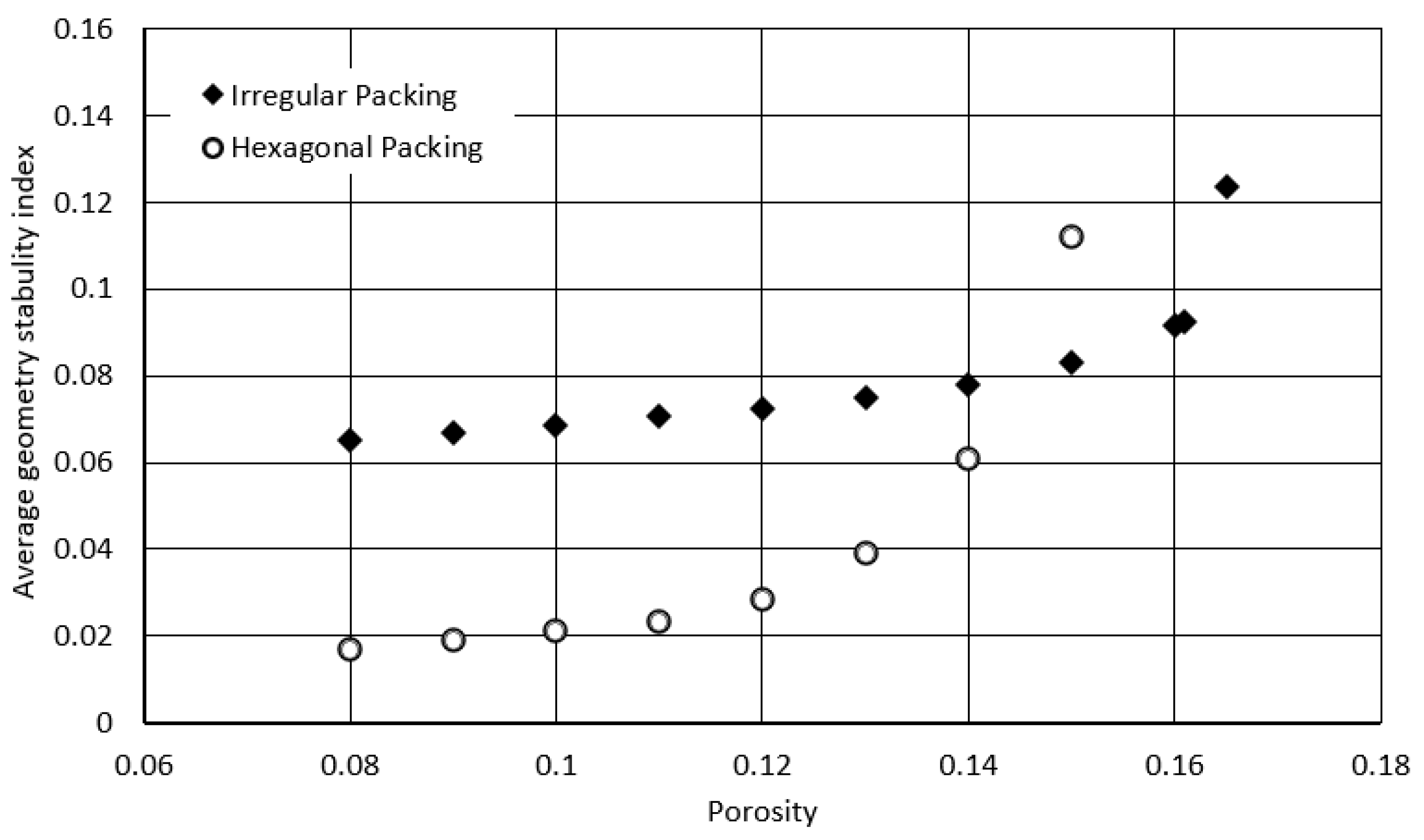
Figure 16 shows that the relationship between porosity and λ is less well defined and that hexagonal packing leads to a more stable configuration for a given porosity.

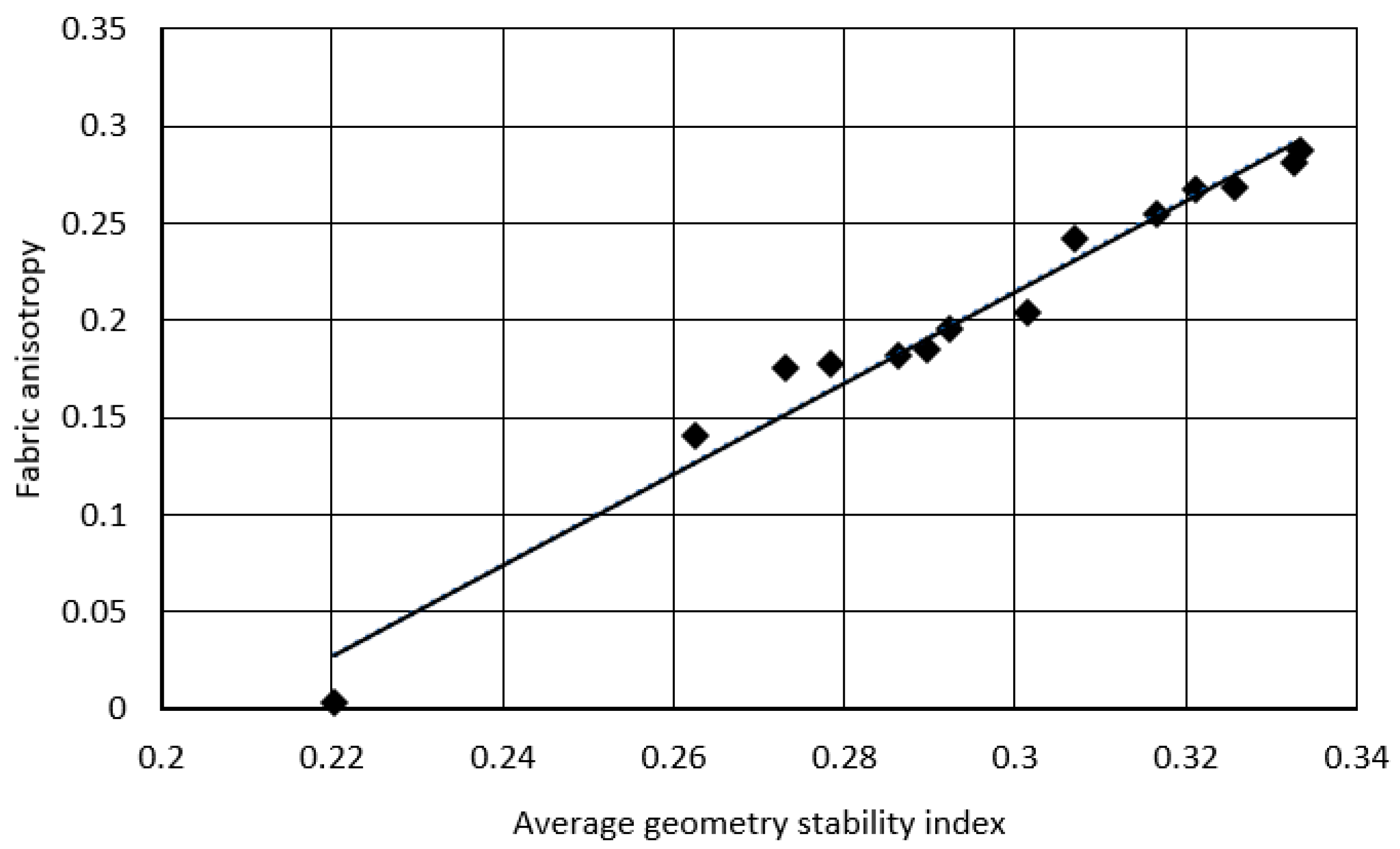
Figure 9 and Figure 14 suggest that there is a relationship between fabric consistency and λ and Figure 17 shows that the fabric anisotropy is linearly related to the average geometric stability index. However, unlike fabric anisotropy, λ can be used at particle level to show the onset of instability (Figure 12). Figure 18 qualitatively compares the volumetric behavior observed by (Wu et al., 2020) [29] and the present work under shearing. The different between the produced macro mechanical behavior of these two works is mainly due to the interparticle properties and strain rate. They applied 5%/min as strain rate. The bigger the value of strain rate, the higher peak stress and residual stress would be achieved.

8. Conclusions

The macro mechanical behavior of granular system is a function of individual particle stability. Although the fabric quantities such as average coordination number and fabric anisotropy are able to estimate the bulk instability, they cannot evaluate the localized particle instability. The conceptual and mathematical development of the geometrical stability index were introduced in this paper to count for the particle instability. An algorithm is developed to determinate the new term and 2D-DEM biaxial simulations were carried out to demonstrate the correlations between the geometrical stability index and the macro mechanical behavior of the system. It was possible to show:

• The development of a shear band with associated turbulent shear by observing the development of the geometric stability index;
• That the index varies with type of packing and, since most soils are irregular packings of randomly sized particles, the initial geometric stability index is always greater than zero (the case for an ideal stable configuration);
• The average geometric stability index increases until the peak stress ratio and then reduces to a constant value at critical state;
• The average geometric stability index for a volume of soil is simply related to the fabric anisotropy and coordination number but, unlike these two fabric quantities, the geometric stability index can be assessed at particle level to show the development of discontinuities.

This helped to confirm the effectiveness of the newly developed fabric term for describing microstructure of the particulate system.