Review

Results of Application of Artificial Neural Networks in Predicting Geo-Mechanical Properties of Stabilised Clays—A Review

Faculty of Environment and Technology, University of the West of England, Bristol BS16 1QY, UK
*
Author to whom correspondence should be addressed.
Geotechnics 2021, 1(1), 147-171; https://doi.org/10.3390/geotechnics1010008
Submission received: 24 June 2021 / Revised: 8 August 2021 / Accepted: 11 August 2021 / Published: 17 August 2021

Abstract

:
This study presents a literature review on the use of artificial neural networks in the prediction of geo-mechanical properties of stabilised clays. In this paper, the application of ANNs in a geotechnical analysis of clay stabilised with cement, lime, geopolymers and by-product cementitious materials has been evaluated. The chemical treatment of expansive clays will involve the development of optimum binder mix proportions or the improvement of a specific soil property using additives. These procedures often generate large data requiring regression analysis in order to correlate experimental data and model the performance of the soil in the field. These analyses involve large datasets and tedious mathematical procedures to correlate the variables and develop required models using traditional regression analysis. The findings from this study show that ANNs are becoming well known in dealing with the problem of mathematical modelling involving nonlinear functions due to their robust data analysis and correlation capabilities and have been successfully applied to the stabilisation of clays with high performance. The study also shows that the supervised ANN model is well adapted to dealing with stabilisation of clays with high performance as indicated by high R2 and low MAE, RMSE and MSE values. The Levenberg–Marquardt algorithm is effective in shortening the convergence time during model training.

1. Introduction

Expansive clays at shallow depths and other poor ground conditions are common problems faced in geotechnical engineering, and these problematic soils pose enormous challenges to the proposed infrastructural development [1,2]. Oftentimes, the option of soil replacement is not economical, and there is a need to perform some form of ground improvement or stabilisation prior to construction [3]. Soil stabilisation may be done chemically or mechanically, depending on the peculiarity of the problem at hand. However, the treatment of most expansive clays will involve the use of chemical stabilisation. Irrespective of the method used, it becomes imperative to investigate the performance of such stabilised soils using key parameters of the soil such as Unconfined Compressive Strength (UCS), Maximum Dry Density (MDD), Optimum Moisture Content (OMC), California Bearing Ratio (CBR), Plasticity index (PI), Liquid Limit (LL), Plastic Limit (PL), grain size, specific gravity GS, etc. [4,5,6,7,8]. These parameters are most times influenced by several variables leading to a multi-variable problem for which researchers have used several statistical methods to analyse, investigate and model trends using laborious mathematical processes involving multivariable regression analyses.
The Artificial Neural Network (ANN) is an emerging trend in dealing with ground improvement involving weak clays. ANN is a computing tool with its architectural concept drawn from that of the biological brain [9,10,11]. Like other artificial intelligence applications or machine-enabled activities, the application of ANN in geotechnical engineering with regards to soil stabilisation is to overcome the supposed complexities and shortcomings of traditional methods in other to save time and resources while obtaining more reliable results. This study explores the usefulness of ANN as a stand-alone machine learning tool in the stabilisation of expansive clays and evaluates its capability in the development of useful mathematical models for the performance evaluation of key properties of stabilised clays. Previous experimental studies are reviewed with a view of assessing the state-of-art in terms of model development, training and performance evaluation.

1.1. Artificial Neural Network

ANN as a branch of artificial intelligence is simply an automated optimisation system capable of learning the relationship and inter-dependencies between multiple input variables of a given system and modelling such relations (trends and patterns) in the form of mathematical functions for easy prediction [12]. ANN has been successfully used in the study of complex systems to identify patterns and model real-life problems relating to complex behaviours involving nonlinear functional relations. The capability of ANN to discover the mapping between several domains of data has drawn the interest of many researchers in geotechnical engineering [13]. ANNs are classified based on numerous criteria such as the learning condition (supervised and unsupervised networks), based on model topography (feedforward or recurring networks), based on a number of hidden layers (shallow or deep networks), based on training algorithm (Back-Propagation Networks, Hopfield Networks, Self-Organizing Map Networks [14]. This paper simplifies the underlying concepts of back propagation ANN models and explores its applicability in modelling the behaviour of stabilised clays viz a viz predicting the response of key soil parameters in other to clear the wide-spread complexities and misconceptions associated with the method and to encourage its use in soil stabilisation problems for more reliable solutions.

1.2. Components of Artificial Neural Network

Neurons and Edges

ANN building blocks are a collection of neurons (nodes) and links mimicking the biological neural network, as shown in Figure 1. The neurons are linked to other neurons by edges and are connected to others so that results from preceding neurons might automatically become inputs for succeeding ones, thereby creating the network. These neurons are the data collection or processing points in the network. Here, signals (input) are processed and transferred to other neurons through the connecting links with each neuron generating a unique output that may become inputs to multiple neurons. In this current subject area of application, these inputs would be laboratory results of key soil parameters described as the dependent variables. The input value of a given neuron is simply obtained by computing the weighted sum of the inputs from connected neurons with the addition of a bias [15,16]. This output of the weighted summation then becomes the input for the activation function- a linear or non-linear function [17,18].
Edges are the links or connections between neurons and convey signals with associated weights depending on the influence of the input from such a link on the output of a given neuron [19]. Inputs parameters with greater importance are assigned a higher weight than those with lower importance [20]. For example, in a soil classification problem, the weights will be dependent on the contribution of the features in determining the class of soil [21]. In a typical perceptron, as in Figure 2, the connection weights can be represented as Wj, which describes the importance of the connection.

2. Materials and Methods

The propagation function [20] computes the weighted summation of inputs from each preceding neuron with the addition of a bias term to create an activation that is utilized by the activation function in computing the output signal. For a typical case such as represented in Figure 2, G (Ij) is the activation function where Ij is the propagation function defined in Equation (1) [22,23]. The activation function could be any of binary step function (Equation (3)), logistic function (Equation (4)), hyperbolic function (Equation (5)), Gaussian function (6), etc. [12].
I j =   Ø j + i   = 1 n W ji ×   X i
W ji is the associated weights of the connections.
X i are the input data.
Ø j is the threshold or bias.
n is the number of inputs.
The connection weights, Wji, are continuously adjusted for each training iteration step using the expression below [24].
W j i m = W j i m 1 +   β ε j X i + δ W j i m 1
In Equation (2), δ W j i is the change in the weight of a given connection, β , ε j   and   represent the learning rate, the error in a neuron’s output and the momentum, respectively, while m is the iteration number. The momentum is used in factoring the weight correction and plays an important role in model training in the sense that too large values cause the model to skip the optimum values of the weight, causing oscillations. On the other hand, too small values will result in delayed convergence between predicted and experimental values [25].
An activation function, such as the binary step function, expresses the output of a given neuron as either of 0 or 1 depending on the input x and is given here as Equation (3).
g ( I j ) = { 0 ,   w h e n   I j < 0 1 ,   w h e n   I j > 0
The binary function due to the gap in the output (only 0 and 1) is unsuitable for training algorithms, which rely on the derivatives of the activation functions [26]. The logistic function also limits the output of a neuron to 0–1 and is expressed by [27].
g ( I j ) =   1 ( 1 + e I j )
The hyperbolic tangent function, as shown in Equation (5), is also a commonly used activation function in ANN [28], and it limits the output of a neuron to −1 and 1. The Gaussian function is another commonly used activation function that defines the normal distribution of a given random input variable about its mean, [29] as presented in Equation (6).
g ( I j ) = e I j e I j e I j + e I j
g ( I j ) = ( 1 σ 2 π ) e ( ( I j µ ) 2 2 σ 2 )
where σ and µ are the standard deviation and mean, respectively.

2.1. ANN Architecture

Deciding the ANN topography is a critical part of the model development and involves an iterative trial and error process (training) [17,30,31,32]. In most studies, an initial model topography is assumed and trained while monitoring the performance of the model using predefined statistical measures such as coefficient of determination (R2), root mean square error (RMSE), mean average error (MAE) and mean square error (MSE). The hyperparameters are continuously modified, and the model retrained until an optimum model architecture is obtained with the lowest error and highest R2 [11,33,34,35]. This training, in simple terms, is “showing the network an example” of the problem using experimental input and output data. Many training algorithms exist; quasi-newton backpropagation, Bayesian regularization backpropagation algorithm, gradient descent, Levenberg–Marquardt optimization, etc., but the process is similar and begins with feeding the model with a quality dataset and allowing the system to process this data in order to learn the relationship between the variables and hence generate weighted associations between the data within the network and predict the result. The predicted result is then compared with the experimental result to evaluate the error, which is then used to modify the weights of the connections by a reverse error minimization process using a chosen cost function. The process is repeated until there is an insignificant change in the output of the cost function [36,37]. Based on the performance of various models with different hyperparameters, the best model topography is then selected.

2.2. Feedforward and Recurring Networks

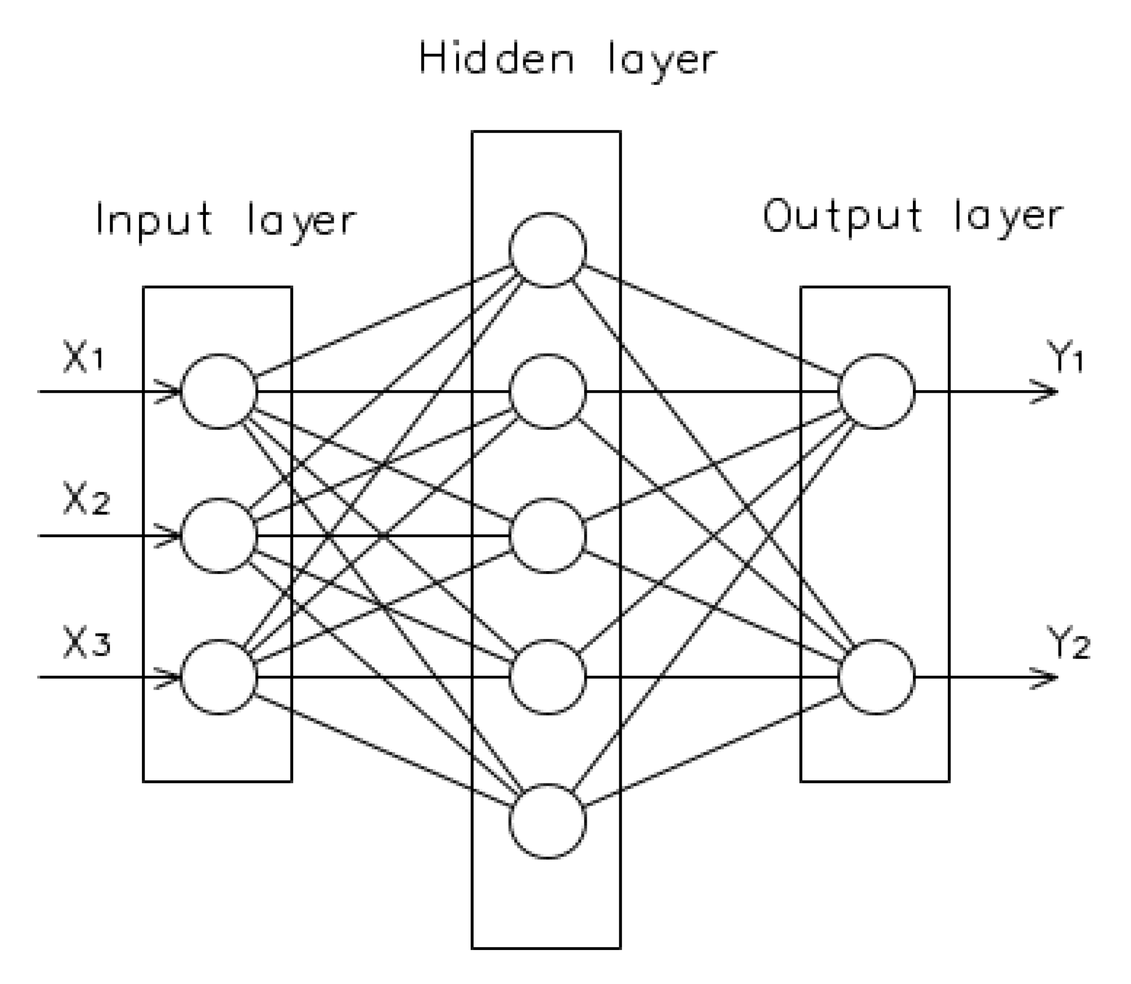
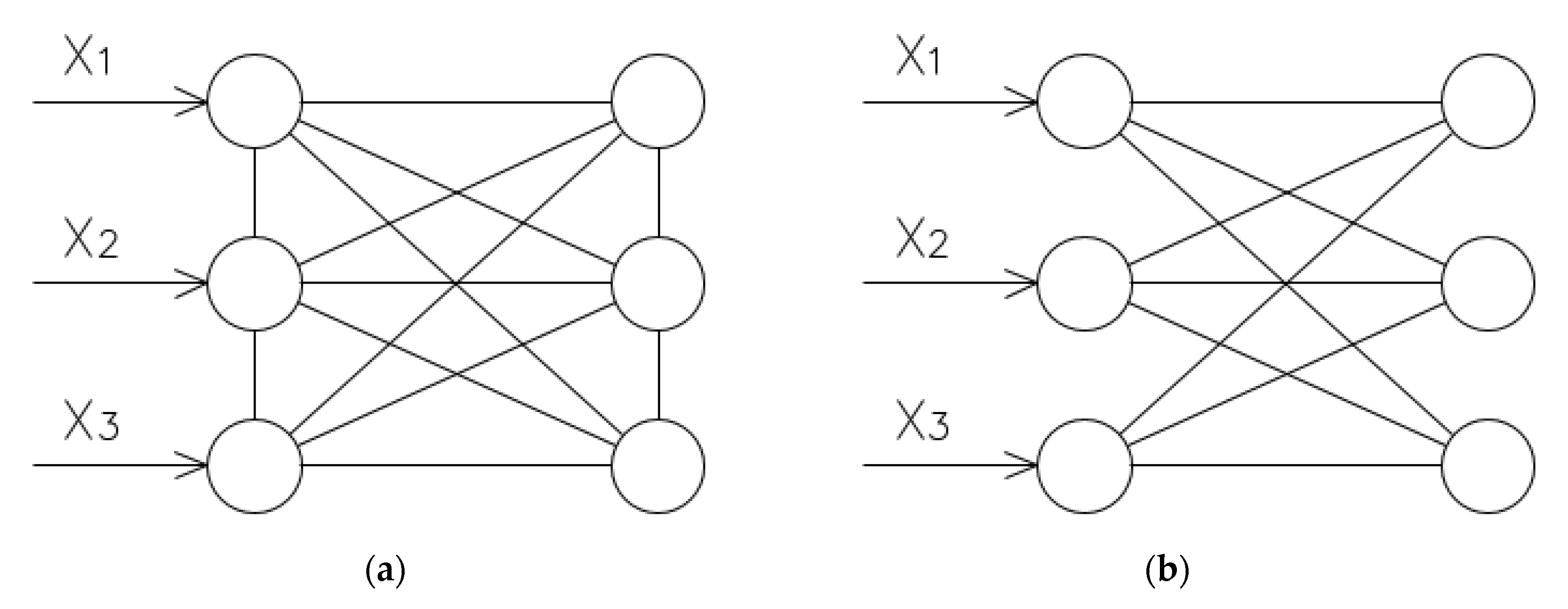
The ANN topography is such that the neurons are grouped into layers, namely input layers and output layers, and in some cases, there is a need to include hidden layers between the input and output layer, making a multilayered perceptron neural network model in order to create sufficient degrees of freedom to avoid overfitting. The hidden layer could be made one layer (shallow networks), as shown in Figure 3, or multiple layers (deep neural network, DNN) [38]. In addition, the connections between layers could be in such a way that a neuron in one layer could be connected to all neurons in the succeeding layer and is said to be fully connected, resulting in a larger number of neurons in the succeeding. Additionally, the models could be organized such that multiple neurons in a layer are connected to a single neuron of the succeeding layer. The latter condition is said to be a pooled connection and is synonymous with a lesser number of neurons in the succeeding layer [39], even though one may be tempted to believe that a larger number of neurons will always result in a better prediction using ANNs. However, the optimum number of neurons will depend on several factors such as the amount of data and the complexity of the relationship. In certain types of NNs, such as the Deep Neural Network, the number of neurons has a lesser effect on the overall performance of the network than the number of layers [12], and DNNs with more hidden layers have been shown to yield more results than shallow networks (network architecture with a single hidden layer). However, the number of hidden layers to be used in each network will depend on the complexity of the mapping between input and output domain, the quality and the amount of data [40]. Additionally, even though it is expected that a greater number of experimental datasets used in training the model will improve the performance of the model, recent studies have shown that it might be advisable to use fewer experimental datasets of high quality than a large amount of experimental data which may be prone to errors [12]. Moreover, the quality of the output is dependent on how the input database is utilized in the training. In terms of the way data is transferred from one layer of the network to another, one can generalize that there are two broad categories of ANN architecture—the recurring network and feedforward network. In the recurring network, there is a connection between neurons of a given layer and that of preceding and/or succeeding layers, forming a loop and allowing an input to be processed many times by the same neuron. Conversely, in the feedforward network, neurons in each layer are only connected to neurons in other layers as presented in Figure 4.

Data Preprocessing

The input dataset used to develop ANN models for geotechnical engineering problems will comprise of various ranges of input variables because the ANN neurons connection weights are representatives of the importance of the variables. The weights of the connections are influenced by the Euclidean distance which for any given points, y1 (x11, x21, x31, …, xn1) and y2 (x12, x22, x32, …, xn2) in a data space can be expressed as Equation (7). Therefore, in order to ensure that proper significance is attributed to the features, it is imperative to scale the features. Feature scaling can be achieved using methods such as standardization (Z-score normalization) or the max-min normalization method. For standardization, the feature X i is expressed in its standardised form as in Equations (7) and (8) below.
d e = ( x 12 x 11 ) 2 + ( x 22 x 21 ) 2 + + ( x n 2 x n 1 ) 2 X s =   X i μ σ
X n o r m =   X i X m i n X m a x X m i n
In Equations (7) and (8), X s is the standardised value of X i , μ is the mean and σ is the standard deviation. The input variables can also be scaled using the max-min normalisation to achieve the same purpose using the expression, where X n o r m is the normalised value and X m i n and X m a x are the minimum and maximum values, respectively.

3. Selecting Design Parameters for ANN in Soil Stabilisation

The training of the neural network is actually the process of selecting or ‘designing’ the best network model parameters (hyperparameters). However, there is a start point where a first architecture is proposed. Selecting the right number of neurons in the hidden layer is critical as it influences the performance of the network. Too few a number of neurons in the hidden layer can lead to underfitting. In this case, the training data presents a more complex problem than the network is modelled to handle. For some problems, increasing the number of neurons by introducing additional features can make learning easier for the model and resolve the problem. In some other cases, for example, in some geotechnical applications, the input parameters of interest may have been predetermined and measured, and this option may not be feasible. Alternatively, increasing the number of hidden layers and neurons may be helpful, but again, if the number of neurons becomes excess, this leads to overfitting. In this case, the model is training on less complex data than it is designed to analyse. The effect is that the model is unable to properly generalize on new data set outside the training data as the weights are not optimally adjusted. Additionally, an excessively high number of neurons in the hidden layer can extend training time and lead to poor training even with a sizable database for training. The goal, therefore, is to find a balance. However, this is not a straightforward process. A good step would be to make a good initialization of the network parameters, and there are several ideas concerning how these parameters can be initialized. Amongst the huge suggestions that are available and, of course, effective under different conditions, one simple empirical rule for selecting the number of neurons in the hidden layer is to use the mean of the number of neurons in both input and output layers. Some other idea involves taken about 60–70% of the total input and output neurons. In general, the idea is to provide a reasonable start so that during the training, the model can be optimised or pruned, and redundant neurons can be removed based on the assigned weights while keeping track of the performance. However, for most regression analyses relating to stabilisation, one hidden layer has been found very effective. In rare cases, two hidden layers have been used, but there are seldom cases where over two layers have been needed in developing reliable predictive models. As shown in the succeeding section, almost all the applications in soil stabilisation have utilised one hidden layer, with one or two utilizing more than one hidden layer.

3.1. Training, Validation, and Testing

As mentioned in the earlier section, the training of most neural networks applied to modelling geomechanical properties of stabilised soils is done under supervised conditions. In this type of training, the supplied data are partitioned, and a part (training dataset) is utilised in learning the relationship between the variables, thereby providing the initial weights. This sample is continuously fed to the network with a view to understanding the data rather than recognizing it. If the network learns progressively, it converges with reduced error after each iteration until a pre-defined error range is attained. The quality of the training dataset influences the convergence of the model [41]. A dataset may lack the necessary independent variables required for the model to understand the data and hence can lead to non-convergence. A very small sample space can lead to the network memorizing rather than learning. Hence, it is important that part of the data is separated to be used in evaluating the training. This is the validation dataset. The major aspect of developing a suitable model would then be to continuously monitor and tweak the number of neurons in the hidden layer, or the number of hidden layers, modify the activation function or even the training algorithm [42]. The model validation utilizes the successive trial of the trained model on the validation dataset [43]. This is an unbiased evaluation of how well the model understands the training data. The final test of the model’s predictive ability is carried out on the test dataset, which was never seen by the model. In some cases, the data are continuously partitioned into two as in cross-validation. The dataset is switched and utilised for training and validation in a crossed pattern.
The performance of models is usually evaluated by using statistical measures such as the coefficient of determination (R2), the mean absolute error (MAE), the root mean square error (RMSE), the mean square error (MSE) and others. The R2, MAE, RMSE and MSE expressions are defined in Equations (9), (10), (11) and (12), respectively.
R 2 =   ( 1 n ( y exp ( i ) y ¯ e x p ) ( y p r e ( i ) y ¯ p r e ) 1 n ( y exp ( i ) y ¯ e x p ) 2 1 n ( y pre ( i ) y ¯ p r e ) 2 ) 2
MAE = I n ( y exp ( i ) y pre ( i ) )
RMSE =   1 n   x   1 n ( y exp ( i ) y p r e ( i ) ) 2
MSE = 1 n   x   1 n ( y exp ( i ) y p r e ( i ) ) 2
For which y exp ( i ) and y pre ( i ) are experimental and predicted values of a given dependent variable, while y ¯ p r e and y ¯ e x p are the mean values of the predicted and experimental values.

3.2. Estimating the Amount of Training Data

Determining the sample size required for successful model training is a vital step in successful model development. A common start-off point is the “rule of ten”, which proposes that the training sample size is taken as not less than ten times the number of network parameters. The number of parameters may be estimated as the number of edges or connections, including biased neurons. It is expected that the performance of the model would improve with increasing sample size following a power function up to a point is reached where there is no significant increase in performance. Usually, in practical situations, the data set is split into the ratio of 70%:30% or 80%:20%, where the higher percentage is that of the training sample space. Although this split is only important with a relatively low sample size. The underlying idea is to make available sufficient example data with which the network is trained and evaluated. Too little training data will result in a higher variance of the network parameters. Additionally, two few testing data will create higher variance during the evaluation of the performance of the model.

4. Application of ANN in Predicting the Properties of Stabilised Clays

The variability of soils following uncontrollable and imprecise chemical and mechanical processes of their formation makes it very complex to predict their behaviour even in the natural state. Several mathematical and graphical models have been proposed for use in modelling the post-stabilisation behaviour of treated clays through the prediction of various engineering parameters for the purpose of design and construction. These methods rely on laboratory results of a few samples with which in-situ post-stabilisation behaviour is to be predicted. However, in many cases, the post-stabilisation behaviour of any soil will be dependent on multiple variables such as curing time, curing duration, soil type, binder content, curing temperature, moisture content, compaction method and effort, plasticity, etc., which are key and influence the dependent variables [44,45]. The large variability of input parameters, the extensive laboratory experiments required and the unknown relationship between the variables put together makes it even more complex to predict the behaviour of the soils [46,47]. In other to simplify the problem, many studies tend to concentrate on a set of few parameters and employ simple mathematical models to map the domains of input to our variables. An example of such simplified mathematical models is the multiple linear regression model, which, for a given set of features x 1 n ,   x 2 n , x 3 n ,   ,   x m n , can be related to its dependent variable as stated in Equation (13) below [23].
y = β 0 + β 1 x 1 n + β 2 x 2 n + β 3 x 3 n + β 1 x m n + ε
where β 0 ,   β 1 , β 3 ,… β n are the coefficients, and ε is the error.
ANN application has shown good results in terms of the prediction of engineering parameters of stabilised soils for various purposes. ANN’s ability to learn the relations between a wider and more complex set of experimental variables and map these variables to the target output domain using well-adjusted weights makes it a more reliable tool in the prediction of the in-situ post-stabilisation behaviour of treated clay soils. In addition, the ability of ANNs to simultaneously handle multiple dependent and independent variables using the same experimental dataset and its adaptability in finding correlations for highly non-linear data, which are characteristic of many civil engineering problems, makes it more advantageous over traditional regression analysis [48,49]. A review of studies modelling various soil properties is presented in the subsequent sections. The review is in a bid to explore the input parameters considered in the study, the number of data utilised in model development, the training algorithm utilised, the hyperparameters of the model, the model performance and, finally, the results or predictive models developed.

4.1. Unconfined Compressive Strength

ANN has been employed in tracking and modelling the UCS of geopolymer stabilised clays [50]. In the study, ground granulated blast furnace slag (GGBS) and pulverised fly ash (PFA) were considered as binders for the improvement of the compressive strength of three clays with varying properties. The soil characteristics such as liquid limit (LL), plastic limits (PL), etc., were evaluated according to the Indian standards and, in combination with key experimental variables, were utilised as input data for the ANN model development. Eight input variables namely, LL, plasticity index (PI), GGBS content, PFA content, the molarity of alkaline activator used (M), the ratio of the activator to the binder, the ratio of sodium to aluminium in the activator–binder mixture (Na/Al), the ratio of silicon to aluminium in the activator–binder mixture (Si/Al), and 28 days UCS, were considered. A multi-layered perceptron ANN model was chosen with one hidden layer to study the experimental data. The optimum architecture was selected by varying the number of neurons in the hidden layer while evaluating the performance of the model and was obtained as one hidden layer with nine neurons. The ANN showed a better ability to learn the relationship of the data set, as shown in Figure 5.
From Figure 5, it is obvious that almost all data points are within the 99% confidence limit. The line of best fit is almost aligned with the line of equality at which all experimental observations and predicted values are the same. Table 1. compares the performance of the ANN model with that of a multivariable regression analysis (MVR) on the same data set. It is obvious that ANN performed better at correlating the independent variables and their influence on the UCS of the stabilised soils.
Expansive soils are known for their vulnerability to significant volume changes with moisture due to their high plasticity properties. Table 2 shows the classification of expansive clays according to the Building Research Establishment (BRE) based on a modified plasticity index.
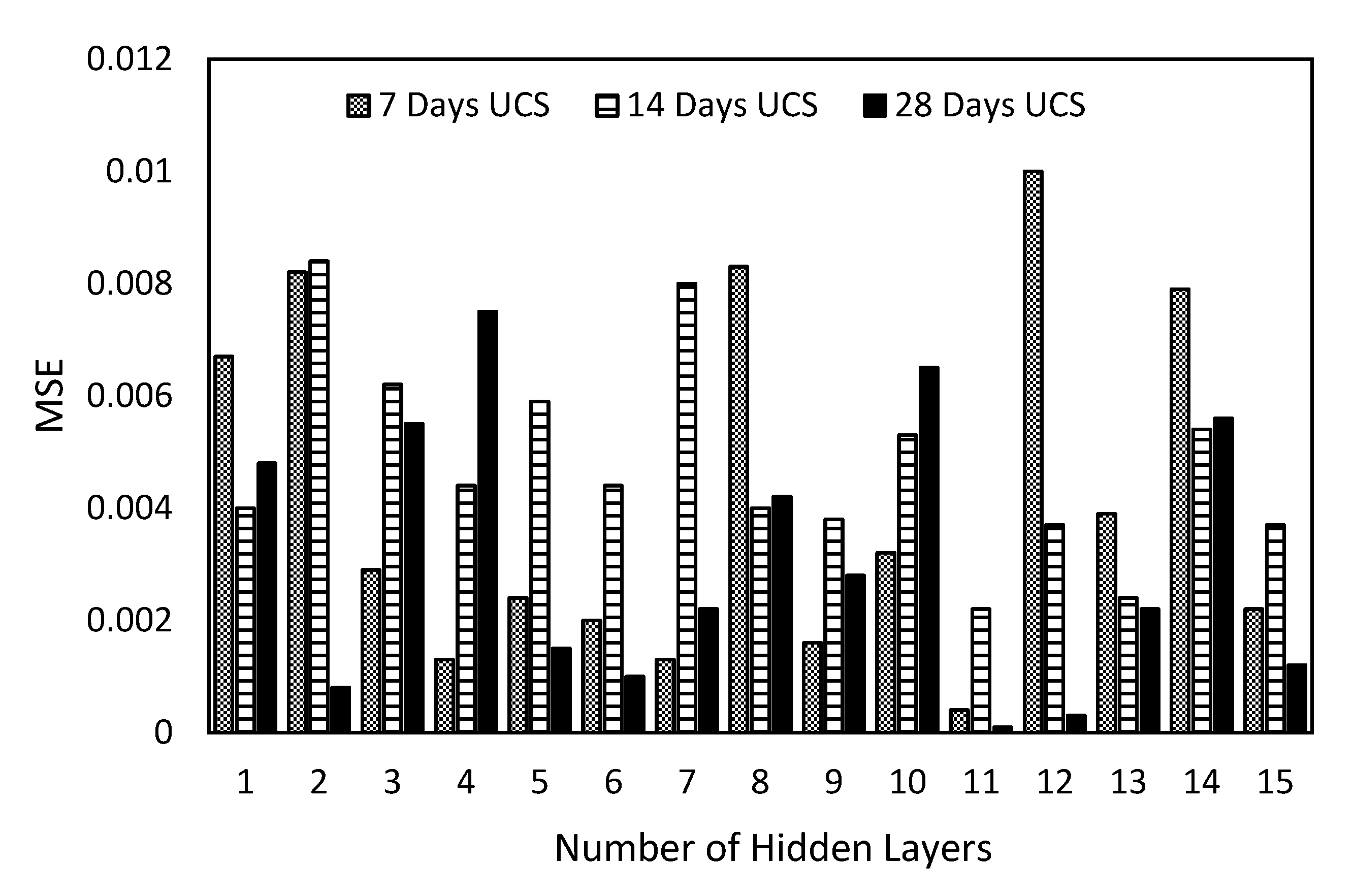
In another study, ref. [52] employed a feedforward ANN model in studying the UCS of expansive clays stabilised with cement-kiln dust (CKD). The liquid limit, plastic limit and plasticity index of the clay were determined to be 48.2%, 27.2% and 21%, respectively. The expansive clay is characterised by a free swell of 80%. The natural and stabilised clay samples were subjected to compaction and UCS test in accordance with [53,54]. Three ANN models were developed with a total of eight input variables, namely specific gravity (Gs), linear shrinkage (LS), coefficient of uniformity (CU), coefficient of gradation (CC), LL, PL, optimum moisture content (OMC), and maximum dry density (MDD) for three UCS outputs (7, 14 and 28 days). A total of 72 data sample data were utilised in model development. The ANN model topography consisted of one input layer with eight neurons and one output neuron (the UCS value). However, the number of hidden layers was varied in order to determine the optimum number of neurons in the hidden layer. Figure 6 shows the performance of the trial models.
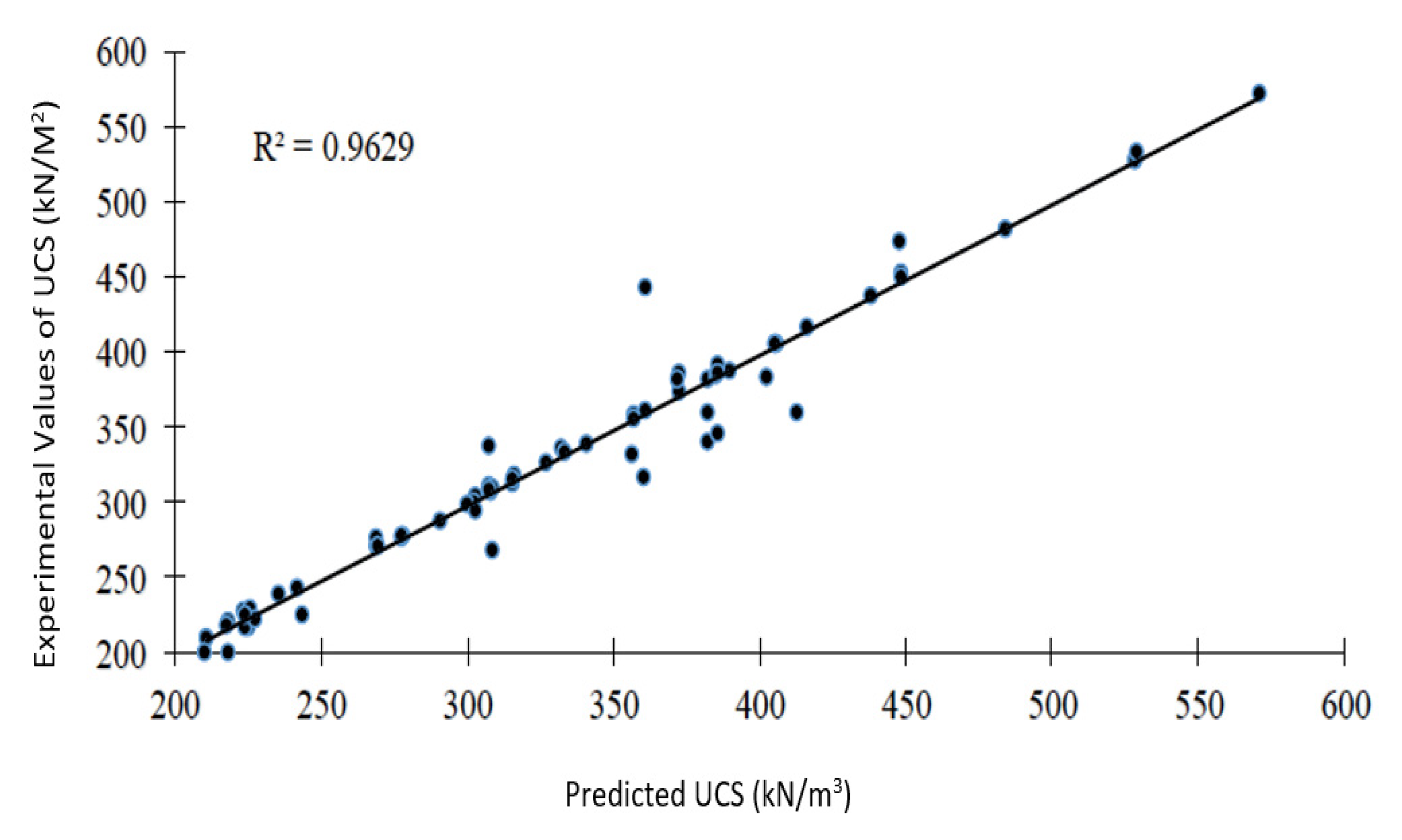
The optimum model was found to be of nine neurons in the hidden layer based on lowest MSE. The authors of [52] suggest that the MSE is a more reliable parameter for network selection when R values alone become insufficient for optimum network selection. The results of the analysis showed that the ANN model was able to predict the variation of UCS as a function of the predictor variables with a high correlation coefficient, as seen in Figure 7.
The study reveals a high correlation between experimental values and ANN predicted values. The high correlation coefficient with low RMSE confirms the performance of the model.
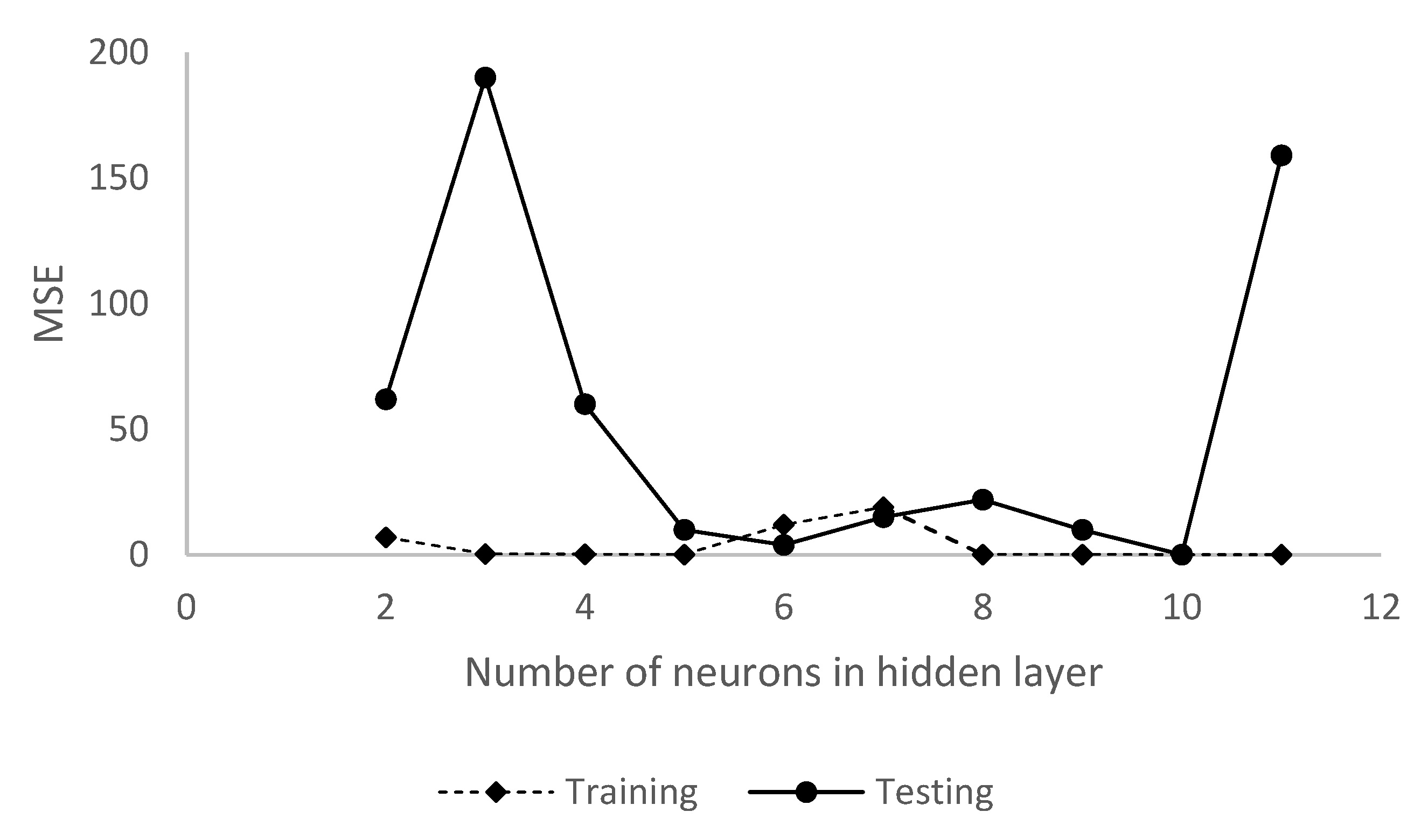
Moreover, the authors of [55] conducted an experimental investigation on the suitability and performance of kaolin clay stabilised with fly ash (PFA), rice husk ash (RHA) and cement. The improvements in the soil were ascertained by considering the increase in the UCS. The LL, PL, and PI of the unstabilised kaolin clay were determined as 43.3%, 19.5% and 23.8%. The input variables considered for the correlation were clay content, RHA content, cement, PFA content and curing duration. The number of neurons in the hidden layer was selected manually and varied while evaluating the performance of the model using the MSE. Figure 8 shows the variation of MSE and the number of neurons in the hidden layer.
As seen in Figure 8, the optimum model performance was found at 10 neurons in the hidden layer based on Levenberg–Marquardt algorithm. The results of the analysis using the optimized model showed a good correlation between the datasets. The predictive model developed from ANN is given in Equation (14).
U C S m U C S C 7 = 1.003 + 1.568 ( C l a y 100 ) 2 + 2.477 ( P F A 100 ) 0.5 + 2.287 ( R H A 100 ) 0.5 + 6.731 ( C e m e n t 100 ) 0.5 + 0.017 C d
where U C S m is the dependent variable to be estimated and represents the UCS for a given combination of independent variables. A comparison of ANN performance with multivariable regression analysis further proves ANN’s advantage, as shown in Table 3. ANN has been described as a black box since it is difficult to predict the way the predictive model will be selected. However, sensitivity analysis can be carried out in determining the influence of the input variables on the target variable.
In a separate study, [56] investigated the performance of stabilised soils with a view to predict the effects of dynamic disturbance on already stabilised soils. The study was to understand the effects of transportation and compaction on strength recovery of already setting stabilised soft clay. Hence, stabilised soil samples were agitated and compacted after curing for some days to simulate the disturbed sample. The UCS was utilised as a performance evaluation parameter. The soils were treated with varying quantities of cement. A kaolin clay with liquid limit, plastic limit and plasticity index of 77.5%, 30.3% and 47.2%, respectively. Ordinary Portland cement was used as a binder for different ratios by mass of dry soil. The UCS test was conducted according to ASTM D2 166-06. It was required to estimate the influence of disturbance on the UCS in terms of an increase factor. ANN was employed in correlating the predictive variables and the dependent variable. A total of 80 experimental data points were generated from combinations of input variables, namely curing duration and compaction energy. The trial and error method was utilised in determining the network topography. However, the performance of one hidden layer was unsatisfactory due to high errors and low R2. The optimum network model was taken as two hidden layers with eight neurons each. The result of the analysis showed a good understanding of the relationship and modelling of the increase factor with a high coefficient of determination and low error. As seen in Figure 9, there is a close approximation of the UCS by the ANN model. The prediction and experimental values are clustered around the line of equality for all three conditions of training, validation and testing.
The UCS of cement stabilised clays was investigated by [57] in order to find a relationship between the several key variables. Different types of cement were utilised to study the effects of cement type on the UCS. The soil under investigation was collected at various depths below the ground surface to also study the effect of confining pressure on the strength of the stabilised soils. Three machine learning algorithms were utilised. ANN was used in correlating the predictive variables. A total of 216 experimental data points were generated from various combinations of fourteen input variables, namely soil type, moisture content (MC), bulk density (We), the mass of cement (CM), sample diameter (DI), the length of the sample (L), the cross-sectional area of the sample (CA), the volume of the sample (SV), the depth of sample collection (D), the mass of the sample (MS), sample density (DS), curing condition (CD), curing time and cement type (CT). ANN training was done using the Quasi-Newton method, Stochastic Gradient Descent and Adam in order to select the optimal hyperparameters for the ANN topography. The dataset was divided in the ratio of 80% and 20% for training and testing. Performance evaluation of the developed ANN model showed a good correlation. ANN performed better than the other machine learning algorithms. The high number of neurons in the hidden layer may be due to the multiple dimensions of the input vector in the sample dataset. The study showed that ANN could be utilised effectively for stabilisation problems to track and model a wide range of independent variables.
To alleviate the difficulties associated with the need for continuous experimental determination of UCS, ref. [58] employed machine learning in analysing and modelling the performance of stabilised dredged sediments. A total of 51 experimental datasets were collated from existing literature for the development of the ANN model. The input predictive variables were percentage moisture content (MC), cement content, air foam content, and waste fishing net content. The ANN model to topography was initialized to two hidden layers while varying the number of neurons in order to find the optimum model. This approach has been taken in most soil stabilisation applications. The optimum ANN architecture was made up of two hidden layers with 12 and 10 neurons based on training using the Levenberg–Marquardt algorithm. From the results of the analysis, the model has been able to find the trend within the available training dataset. However, for certain values of the water content, the error was high. For the model to generalize better, a wider training dataset may still be needed. Previous studies have suggested a training dataset at least ten times the network parameters. In a lot of original research on stabilisation, there is usually limited experimental data. A cross-validation approach may be combined for a relatively lower sample size. The statistical evaluation of the performance of the model in training and testing is presented at the end of Section 4.

4.2. California Bearing Ratio

The California bearing ratio (CBR) of soils is of interest in pavement design. Several geotechnical investigations are concerned with measuring the CBR of stabilised soils. The aim of some soil stabilisation is for improvements in CBR to meet the desired outcome. However, the determination of CBR is expensive. It is desirable to be able to correlate and predict CBR from known soil characteristics. A study by [59] involved modelling the CBR of stabilised expansive soils. The expansive clays were treated with lime and quarry dust as a binder. The quarry dust is a by-product of the crushing of rock for aggregates. The characteristics of the expansive clay, such as Atterberg properties, compaction and CBR, were determined following the Indian standards. The stabilisation of the soil was carried out by the addition of lime and quarry dust of different percentages to the soil and tested of CBR at 0, 7 and 28 days. A total of 49 data samples were generated for correlation from the combination of four input parameters, namely LL, PI, OMC and MDD. To develop the required regression models, three ANN models were utilised based on different training algorithms using Differential evolution (DE), Bayesian regularization (BR) and Levenberg–Marquardt (LM) algorithm. The training data was taken as 70% of the 49 data samples, while 30% was utilised for testing. Again, the limitations in the availability of extensive experimental data are seen and may be due to cost implications. However, the Levenberg–Marquardt-trained ANN performed better based on the limited data sample. Additionally, the models showed signs of overfitting, which may be due to insufficient training data. Detailed summary of model performances for the 28-day CBR model is shown at the end of Section 4.
The experimental study by [60] employed ANN in modelling soaked CBR of expansive stabilised clays. The clay was stabilised with varying proportions of coal ash, bagasse ash and groundnut shell ash (GSA) and geogrid layers. The soil classification was conducted in line with Indian Standards. The input variables used were the type of ash, mix proportion, LL, PL, MDD, OMC and the number of geogrid layers. The soil was stabilised with various combinations of the different features to generate 210 data samples, which were utilised in training and testing the ANN model. The optimum model architecture was found to be made of one hidden layer with seven neurons. The model was trained with different algorithms in order to select the best algorithm based on R2 and MSE. The performance of the models based on the training algorithm is given in Table 4.
The Levenberg–Marquardt training algorithm was selected as the best performing based on R and MSE values. The model performed well with good predictive ability. The results showed that the ANN model was capable of modelling the soaked CBR of the stabilised soils. The performance of black cotton soil stabilised with fly ash and geotextile was studied by [61] with a view to develop a regression model for predicting the CBR of stabilised black cotton soil. The soil used in the study was characterised according to Indian standards. The LL and PL of the soil were reported as 47% and 17%, respectively. Additionally, the compaction characteristics were determined using standard proctor compaction tests with MDD and OMC, resulting in 16.26 kN/m3 and 15%, respectively. The ANN models were developed using LL, PL, fly-ash content, OMC, MDD and the number of geotextile layers as input variables, while soaked CBR was the target variable in the output neuron. Different training algorithms were employed while varying the number of neurons in the hidden layer to select the best model architecture. The performance of the models is presented here, as shown in Table 5.
The Levenberg–Marquardt function was adopted based on minimum error and the highest R2. The models performed well with minimum error in relation to a higher coefficient of determination. A regression analysis of the CBR of soils stabilised with lime and rice husk ash (RHA) was carried out by [62]. The LL and PL of the soil were reported as 34% and 20%, with clay and silt content of 20% and 71%. Additionally, the MDD and OMC of the soil were reported as 17.7 kN/m3 and 14.7%, respectively. The CBR test was conducted in line with ASTM D1883 -07. Soaked CBR tests were conducted on 0, 7 and 28 days cured samples. The predictive variables considered in the study were the percentage of RHA, percentage of lime, curing duration, OMC and MDD. The topography of the ANN model was determined by trial and error by varying the number of neurons in the hidden layer. Optimum model topography was found to be one hidden layer and twelve neurons from the R value and MAE. The model performance as per the training data showed higher R and low MAE. The number of data utilised for training is deemed small. The performance of the model in generalizing new data may be affected due to overfitting. This again is a common factor confronting the application of ANN in soil stabilisation studies.
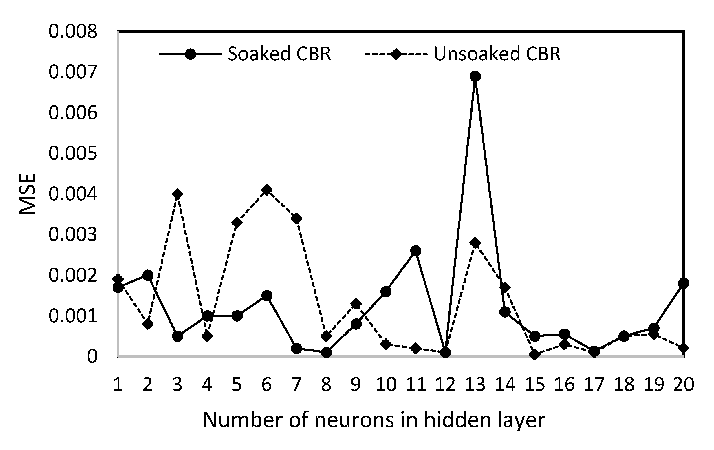
Furthermore, [63] investigated a predictive model for the correlation of soaked and unsoaked CBR of stabilised black clay. The black clay is an expansive clay found in semi-arid regions of tropical and temperate climates. The stabilisation of the clay was done with cement kiln dust as a binder. The characteristics of the soil and cement kiln dust were determined according to the British Standards [53,54]. Eight input parameters, namely PL, LL, specific gravity (GS), linear shrinkage (LS), coefficient of uniformity (CU), coefficient of gradation (CC), OMC and MDD, were utilised in developing 72 data samples for two ANN models; soaked and unsoaked CBR. The model architecture was determined by varying the number of neurons in the hidden layer from 1 to 20 while evaluating the MSE and R values. Figure 10 shows the performance of various model architectures.
The optimum was determined using the lowest MSE value. As seen in Figure 10, for soaked CBR, a model architecture with 8 neurons in the hidden layer was chosen, while 17 neurons in the hidden was optimum for unsoaked CBR. The models performed effectively in correlating and predicting the CBR of the stabilised soils with high R and low MSE.

4.3. Permeability and Resilient Modulus

The permeability of soil is an important property of soil that describes the ease with which water flows through a soil mass. In certain geotechnical applications such as earth embankment and dam designs, it is desirable to be able to model and predict the permeability of the soil. The study by [64] investigated the effects of lime and pozzolan on the permeability of dispersive clays. Dispersive clays are highly susceptible to erosion due to their high sodium ion content, which often leads to structural disintegration into finer particles easily washed away during seepage. The LL and PL of the unstabilised clay were determined as 34% and 17%, while the MDD and OMC were 17.85 kN/m3 and 16.5%, respectively. The clays soil was stabilised with various combinations of lime and pozzolan. Permeability tests were conducted to develop a dataset of 69 samples for the regression analysis. A total of six independent variables were used in the development of the ANN model, including percentage passing 0.005 mm size sieve, PI, MDD, lime percentage, pozzolan percentage and curing time (Cd). To develop the predictive model, ANNs with varying numbers of neurons in the hidden layer were tried. An optimum model with nine neurons in the hidden layer was selected based on low MSE and high R value as with other studies. In line with other studies, 70% of the data was used for training, 15% for testing, and 15% for validation. The performance of the model was satisfactory in terms of low MSE and high R values.
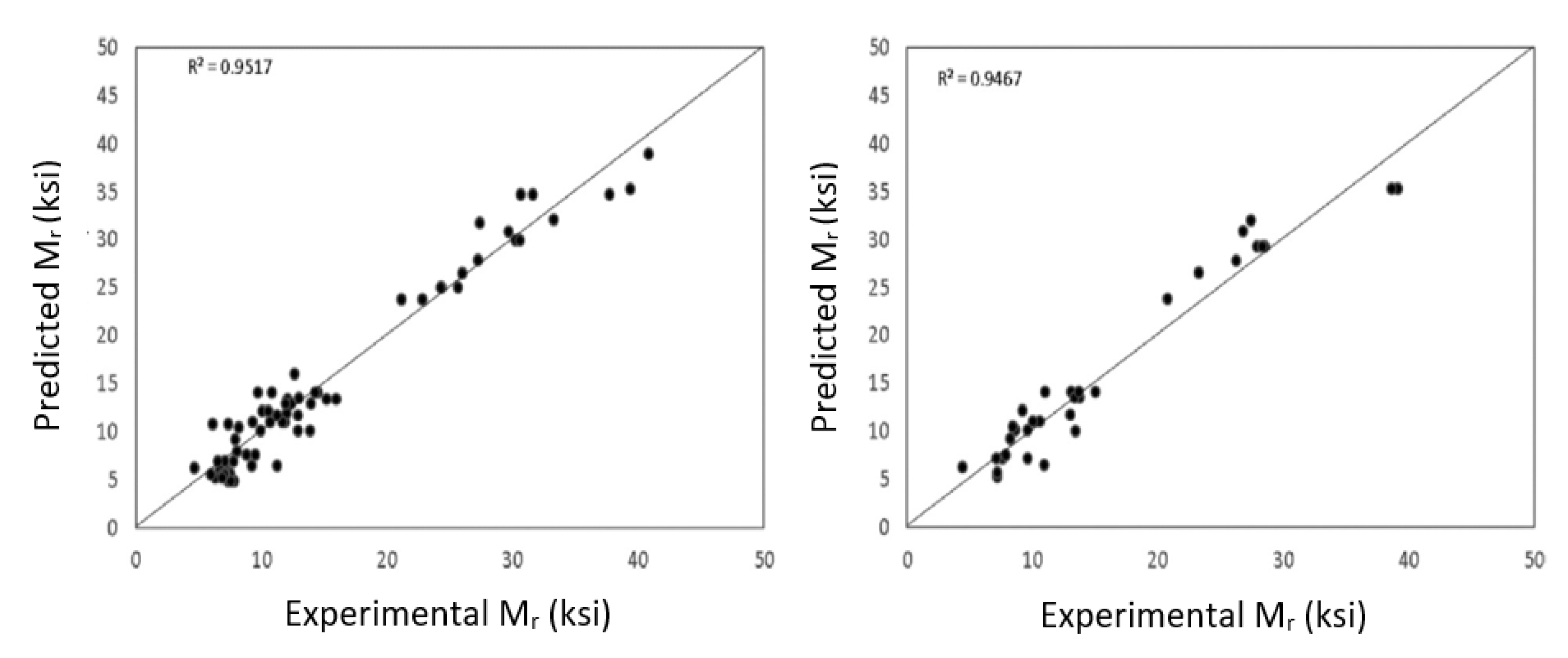
The resilient modulus of soil is also a useful parameter in pavement design. Few studies are available on the resilient modulus of soils. Hence, predictive models for resilient modulus of stabilised clays are desirable. ANN has also been utilised in correlating and modelling resilient modulus (Mr) of stabilised clays [65]. The LL, PL, particle size and compaction characteristics of four unstabilised soil samples were determined according to ASTM D4318, ASTM D4318, ASTM D422 and ASTM D698. The resilient moduli were determined by subjecting treated samples to cyclic load test according to AASHTO T307 standard method (AASHTO 2003). A total of 125 data samples were generated for ANN modelling. Eight inputs parameters, namely cement content, lime content, PI, silt content, PFA, OMC, MC and clay content, were considered. The trial and error method was used to determine the optimum model as one hidden layer and nine neurons. The performance evaluation was based on R values. The model could predict the resilient modulus with a high correlation. The predicted and experimental values were very close, which was indicative of the accuracy of the developed predictive model. Figure 11 shows the correlation between predicted and experimental data.

4.4. Plasticity Index and Compaction Characteristics

ANN was also utilised by [66] in regression analysis to develop predictive models for MDD and OMC using eight input variables LL, PI, LS, clay-silt ratio, sand content, lime content, cement content and asphalt content in percentage. A total of 192 datasets were obtained from reported laboratory experiments and utilised in training based on gradient descent momentum algorithm for the development of the regression model for MDD and OMC predictions. The optimum model was obtained by trial and error using 52% of the data for training, 24% for testing and 24% for validation. Performance evaluation of the models shows a good correlation as with similar studies. Furthermore, [67] investigated the MDD and OMC of cement stabilised black cotton clay. The clay was treated with various percentages of cement kiln dust (CKD). The input parameters used were LL, PL, specific gravity (GS), linear shrinkage (LS), free swell, grain sizes (D10, D30 and D60), coefficient of uniformity (CU), and coefficient of gradation (CC). Two separate ANN models were developed for MDD and OMC using five and seven neurons, respectively, in the hidden layers. The models were reported to have performed effectively and predicted the MDD and OMC with high correlation and low errors. Table 6 shows detailed results of different ANN models and their performances.

5. Discussions

Problematic clays are commonly encountered in geotechnical engineering practice and will demand extensive ground improvement programs under practical conditions. Undoubtedly, chemical stabilisation involving the use of calcium and non-calcium-based binders have been successfully used to stabilise and improve the engineering properties of clays, making them fit for a specified purpose. The stabilisation process will often require series of detailed laboratory procedures, including sample preparation, curing and testing. This is followed by the analysis of the experimental data, observation of trends, the establishment of the relationship between variables and development of predictive models [68,69,70,71,72,73,74]. In the case of a large collection of data involving multiple variables, it is very tedious to learn the functional relations and inter-variable dependencies without the use of a more sophisticated tool or technique, such as the concept of artificial intelligence.
Reference [68] has observed that ANN’s application in soil stabilisation is a relatively new development. However, the present study shows that it is fast becoming a more reliable tool in the development of predictive models for the prediction of geotechnical properties of stabilised clays. The ability of ANN to learn the functional relations and inter-variable dependencies within large collections of independent variables gives it a major advantage over traditional regression analysis involving cumbersome mathematical procedures. Some studies have utilised a relatively large database of soil properties, as seen in Table 3, and will require a longer analysis time using regression analysis. These traditional procedures become even more cumbersome if a change is made in any variable in the dataset as the analysis must be repeated. However, in using ANN, such changes can easily be accommodated without any repetition, and this gives ANN the advantage of fitting a closer curve on the experimental data for the parameter of interest as a larger dataset encompasses a wider variety of soil responses. Another advantage of ANN is the possibility of modelling multiple dependent or target variables simultaneously. ANN can search the relationship between a given dataset and two or more dependent variables while assigning required coefficients for the various targets. As seen in Table 3, some studies have simultaneously modelled more than one dependent variable and obtained good predictive models for the dependent variables. This, again, is a time-saving advantage.
From Table 3, it can be seen that the performance of the model is not directly proportional to the number of neurons in the hidden layer. However, a sufficient number of neurons based on model training must be allowed for optimum performance and is majorly dependent on several parameters depending on the complexity of the problem investigated. ANN has been successfully utilized in performance evaluation and post-stabilisation behaviour of treated clays with a high degree of reliability. From some of the studies presented in Table 3, statistical evaluation of ANN’s performance show superior modelling capabilities than the usual regression models. The high R2 and low MSE, MAE and RMSE of ANN regression analysis are pointers to its advantage. From the study, it was discovered that most of the ANN models utilized were backpropagation feed-forward networks with one hidden layer. Only two studies [56,58] used two hidden layers for the analysis. Other studies have also pointed out that most regression analyses in soil stabilisation problems are easily solved using a simple architecture of one hidden layer.
In addition, the quality and size of the database used in training contributes to the robustness of the model and enhances its performance in terms of generalisation. As seen in Table 7, many of the studies have used a relatively small dataset for the analysis, and this raises concerns if the models would be reliable under practical conditions.
One major factor may be due to the high cost of conducting geotechnical experimentation. This factor may be more significant in other areas of geotechnical engineering other than soil stabilisation. However, as shown in Table 3, satisfactory performance has also been achieved with a relatively small dataset within the available training dataset.
The capabilities of ANN in soil stabilisation are wide-ranged, including the determination of the optimum mix design for a given additive, the optimisation of soil parameters by adjusting dependent soil properties, predicting the mineralogical composition of stabilised soils, classifying soils based on established criteria and modelling and predicting the performance of stabilised soils. In summary, it is obvious that ANN can be utilised in regression analysis for the development of useful models for modelling the geo-mechanical properties of stabilised clays and indeed in soil stabilisation as a whole.

6. Conclusions

  • The advantages of the artificial neural over traditional regression analysis as applied to stabilisation have been highlighted in the foregoing sections. In a typical field stabilisation project, in order to improve the properties of expansive clays, experimental data are usually generated from several field and laboratory tests to monitor and ascertain the progress made in terms of improvement. These procedures are expensive and time-consuming and may be reduced to a minimum using ANN to predict the field response of the soils. In summary, the following conclusions are made.
  • An artificial neural network is reliable and can be employed in modelling various properties of stabilised clays for easy prediction of soil response while eliminating the need for extensive experimental procedures.
  • Backpropagation feedforward networks are the most used models in dealing with the problem of regression analysis for stabilisation of clays.
  • An artificial neural network should be developed with a relatively substantial dataset to regression models with good correlation. Many of the studies in regression analysis of stabilised clays have used relatively small data sets, although the models have performed well. The ability of the models to generalize can be improved with a larger dataset which fields a wide range of possible soil behaviour for proper training of the model.
  • Shallow networks made up of one hidden layer are the most used ANN architecture in developing predictive models for the prediction of geotechnical characteristics of stabilised clays and in modelling the response of stabilised expansive clays. The Levenberg–Marquardt training algorithm has been reported to be the most used among the studies reviewed.

Author Contributions

Conceptualization, S.J.A. and J.J.J.; methodology, J.J.J. and S.J.A.; software, A.K.; validation, J.J.J. and S.J.A.; formal analysis, J.J.J. and S.J.A.; investigation, J.J.J. and S.J.A.; resources, S.J.A., A.K. and C.A.B.; data curation, J.J.J. and S.J.A.; writing—original draft preparation, J.J.J. and S.J.A.; writing—review and editing, J.J.J., S.J.A. and C.A.B.; visualization, S.J.A., C.A.B. and A.K.; supervision, S.J.A., C.A.B. and A.K.; project administration, C.A.B., A.K. and S.J.A. All authors have read and agreed to the published version of the manuscript.

Funding

This research received no external funding.

Institutional Review Board Statement

Not applicable.

Informed Consent Statement

Not applicable.

Data Availability Statement

Some or all data that support the findings of this study are available from the corresponding author.

Acknowledgments

The lead author is thankful to the Ph.D. supervisory team for their enormous support during this study.

Conflicts of Interest

The authors declare no conflict of interest.

References

  1. Gillott, J.E. Some clay-related problems in engineering geology in North America. Clay Miner. 1986, 21, 261–278. [Google Scholar] [CrossRef]
  2. Das, A.; Roy, S. Effect of Expansive Soil on Foundation and Its Remedies. Int. J. Innov. Res. Sci. Eng. Technol. 2014, 3, 92–95. [Google Scholar]
  3. Balasingam, M.; Farid, S. Interpretation of Geotechnical Properties of Cement Treated Soil; Washington State Department of Transportation (WSDOF): Olympia, WA, USA, 2008; pp. 77–122.
  4. Chew, S.H.; Kamruzzaman, A.H.M.; Lee, F.H. Physicochemical and Engineering Behavior of Cement Treated Clays. J. Geotech. Geoenvironmental Eng. 2004, 130, 696–706. [Google Scholar] [CrossRef]
  5. Abbey, S.J.; Eyo, E.U.; Oti, J.; Amakye, S.Y.; Ngambi, S. Mechanical Properties and Microstructure of Fibre-Reinforced Clay Blended with By-Product Cementitious Materials. Geosciences 2020, 10, 241. [Google Scholar] [CrossRef]
  6. Abbey, S.J.; Ngambi, S.; Olubanwo, A.O.; Tetteh, F.K. Strength and Hydraulic Conductivity of Cement and By–Product Cementitious Materials Improved Soil. Int. J. Appl. Eng. Res. 2018, 13, 8684–8694, ISSN 0973-4562. [Google Scholar]
  7. Eyo, E.U.; Ng’Ambi, S.; Abbey, S.J. Incorporation of a nanotechnology-based additive in cementitious products for clay stabilisation. J. Rock Mech. Geotech. Eng. 2020, 12, 1056–1069. [Google Scholar] [CrossRef]
  8. Eyo, E.U.; Ng’Ambi, S.; Abbey, S.J. Performance of clay stabilized by cementitious materials and inclusion of zeolite/alkaline metals-based additive. Transp. Geotech. 2020, 23, 100330. [Google Scholar] [CrossRef]
  9. Dongare, A.D.; Kharde, R.R.; Kachare, A.D. Introduction to Artificial Neural Network. Int. J. Eng. Innov. Technol. 2012, 2, 189–193, ISSN 2277-3754. [Google Scholar]
  10. Sharma, V.; Rai, S.; Anurag Dev, A. A Comprehensive Study of Artificial Neural Networks. Int. J. Adv. Res. Comput. Sci. Softw. Eng. 2012, 2, 278–284, ISSN 2277 128X. [Google Scholar]
  11. Vastrad, C. Performance Analysis of Neural Network Models for Oxazolines and Oxazoles Derivatives Descriptor Dataset. Int. J. Inf. Sci. Tech. 2013, 3, 1–15. [Google Scholar] [CrossRef]
  12. Stepniewska-Dziubinska, M.M.; Zielenkiewicz, P.; Siedlecki, P. Development and evaluation of a deep learning model for protein–ligand binding affinity prediction. Bioinformatics 2018, 34, 3666–3674. [Google Scholar] [CrossRef] [Green Version]
  13. Lal, B.; Tripathy, S.S. Prediction of dust concentration in open cast coal mine using artificial neural network. Atmos. Pollut. Res. 2012, 3, 211–218. [Google Scholar] [CrossRef] [Green Version]
  14. Chao, Z.; Ma, G.; Zhang, Y.; Zhu, Y.; Hu, H. The application of artificial neural network in geotechnical engineering. International Conference on Civil and Hydraulic Engineering (IConCHE). IOP Conf. Ser. Earth Environ. Sci. 2018, 189, 22054. [Google Scholar] [CrossRef]
  15. Nihat, S.I. Estimation of swell index of fine-grained soils using regression equations and artificial neural net-works. Sci. Res. Essay 2009, 4, 1047–1056. [Google Scholar]
  16. Rani, C.S.; Vaddi, P.K.; Togati, N.V.V.K. Artificial Neural Networks (ANN) for Prediction of Engineering Properties of Soils. Int. J. Innov. Technol. Explor. Eng. 2013, 3, 123–130, ISSN 2278-3075. [Google Scholar]
  17. Kalantary, F. and Kordnaeij, A. Prediction of compression index using artificial neural network. Sci. Res. Essays 2012, 7, 2835–2848. [Google Scholar] [CrossRef]
  18. Singh, V.; Bano, S.; Yadav, A.K.; Ahmad, S. Feasibility of Artificial Neural Network in Civil Engineering. Int. J. Trend Sci. Res. Dev. 2019, 3, 724–728. [Google Scholar] [CrossRef]
  19. Winston, P.H. Artificial Intelligence, 3rd ed.; Addison-Wesley Pub. Co.: Boston, MA, USA, 1992; ISBN 0-201-53377-4. [Google Scholar]
  20. Zell, A. Simulation of Neural Networks, 1st ed.; Addison-Wesley Pub. Co.: Boston, MA, USA, 2003; ISBN 978-3-89319-554-1. OCLC 249017987. [Google Scholar]
  21. Cal, Y. Soil classification by neural network. Adv. Eng. Softw. 1995, 22, 95–97. [Google Scholar] [CrossRef]
  22. Shahin, M.A.; Jaksa, M.B.; Maier, H.R. Artificial Neural Networks-Based Settlement Prediction Formula for Shallow Foundations on Granular Soils. Aust. Geomech. 2002, 37, 45–52. [Google Scholar]
  23. Gunaydin, O.; Gokoglu, A.; Fener, M. Prediction of artificial soil’s unconfined compression strength test using statistical analyses and artificial neural networks. Adv. Eng. Softw. 2010, 41, 1115–1123. [Google Scholar] [CrossRef]
  24. Kerh, T.; Hu, Y.G.; Wu, C.H. Estimation of consolidation settlement caused by groundwater drawdown using artificial neural networks. Adv. Eng. Softw. 2003, 34, 559–568. [Google Scholar] [CrossRef]
  25. Reuter, U.; Sultan, A.; Reischl, D.S. A comparative study of machine learning approaches for modeling concrete failure surfaces. Adv. Eng. Softw. 2018, 116, 67–79. [Google Scholar] [CrossRef]
  26. Snyman, J. Practical Mathematical Optimization: An Introduction to Basic Optimisation Theory and Classical and New Gradient-Based Algorithms; Springer Science & Business Media: New York, NY, USA, 2005; ISBN 978-0-387-24348-1. [Google Scholar]
  27. Hinkelmann, K. Neural Networks. University of Applied Sciences Northwestern Switzerland School of Business. Available online: http://didattica.cs.unicam.it/lib/exe/fetch.php?media=didattica:magistrale:kebi:ay_1718:ke-11_neural_networks.pdf (accessed on 26 April 2021).
  28. Weisstein, E.W. Hyperbolic Tangent. MathWorld—A Wolfram Web Resource. Available online: https://mathworld.wolfram.com/HyperbolicTangent.html (accessed on 26 April 2020).
  29. Squires, G.L. Practical Physics; Cambridge University Press (CUP): New York, NY, USA, 2001; ISBN 978-0-521-77940-1. [Google Scholar] [CrossRef]
  30. Mote, H.; Kumar, S.R.S. Use of Artificial Neural Network for Initial design of steel structures. IOP Conf. Ser. Mater. Sci. Eng. 2019, 660, 12064. [Google Scholar] [CrossRef]
  31. Sildir, H.; Aydin, E.; Kavzoglu, T. Design of Feedforward Neural Networks in the Classification of Hyperspectral Imagery Using Superstructural Optimization. Remote Sens. 2020, 12, 956. [Google Scholar] [CrossRef] [Green Version]
  32. Naidu, K.; Ali, M.S.; Abu Bakar, A.H.; Tan, C.K.; Arof, H.; Mokhlis, H. Optimized artificial neural network to improve the accuracy of estimated fault impedances and distances for underground distribution system. PLoS ONE 2020, 15, e0227494. [Google Scholar] [CrossRef] [PubMed] [Green Version]
  33. Renotte, C.; Wouwer, A.V.; Bogaertst, P.; Remy, M. Neural Network Applications in Non-linear Modelling of (Bio) chemical Processes. Meas. Control. 2001, 34, 197–201. [Google Scholar] [CrossRef]
  34. Zhang, T.; Fell, F.; Liu, Z.; Preusker, R.; Fischer, J.; He, M. Evaluating the performance of artificial neural network techniques for pigment retrieval from ocean color in Case I waters. J. Geophys. Res. Space Phys. 2003, 108, 3286. [Google Scholar] [CrossRef]
  35. Eyo, E.U.; Abbey, S.J. Machine learning regression and classification algorithms utilized for strength prediction of OPC/by-product materials improved soils. Constr. Build. Mater. 2021, 284. [Google Scholar] [CrossRef]
  36. Schmidhuber, J. Deep learning in neural networks: An overview. Neural Netw. 2015, 61, 85–117. [Google Scholar] [CrossRef] [Green Version]
  37. Wald, A. Statistical Decision Functions; John Wiley & Sons: New York, NY, USA, 1950. [Google Scholar]
  38. Ikizler, S.B.; Aytekin, M.; Vekli, M.; Kocabas, F. Prediction of swelling pressures of expansive soils using artificial neural networks. Adv. Eng. Softw. 2009, 41, 647–655. [Google Scholar] [CrossRef]
  39. Ciresan, D.; Meier, U.; Masci, J.; Gambardella, L.M.; Schmidhuber, J. Flexible, High Performance Convolutional Neural Networks for Image Classification. Twenty-Second Int. Jt. Conf. Artif. Intell. 2011, 2, 1237–1242. [Google Scholar]
  40. Sushama, K.; Bindhu, L. ANN Based Prediction of Shear Strength of Soils from their Index Properties. Int. J. Earth Sci. Eng. 2015, 8, 2195–2202, ISSN 0974-5904. [Google Scholar]
  41. Murata, N.; Yoshizawa, S.; Amari, S. Learning curves, model selection and complexity of neural networks. In Advances in Neural Information Processing Systems 5; Jose Hanson, S., Cowan, J.D., Lee Giles, C., Eds.; Morgan Kaufmann: San Mateo, CA, USA, 1993; pp. 607–614. [Google Scholar]
  42. Maind, S.B.; Wankar, P. Research Paper on Basic of Artificial Neural Network. Int. J. Recent Innov. Trends Comput. Commun. 2014, 2, 96–100. [Google Scholar]
  43. Gareth, J. An Introduction to Statistical Learning: With Applications in R; Springer: New York, NY, USA, 2013; p. 176. ISBN 978-1461471370. [Google Scholar]
  44. Pathivada, S. Effects of Water-Cement Ratio on Deep Mixing Treated Expansive Clay Characteristics; The University of Texas at Arlington: Arlington, TX, USA, 2005. [Google Scholar]
  45. Lorenzo, G.A.; Bergado, D.T. Fundamental Parameters of Cement-Admixed Clay—New Approach. J. Geotech. Geoenvironmental Eng. 2004, 130, 1042–1050. [Google Scholar] [CrossRef]
  46. Turk, G.; Logar, J.; Majes, B. Modelling soil behaviour in uniaxial strain conditions by neural networks. Adv. Eng. Softw. 2001, 32, 805–812. [Google Scholar] [CrossRef] [Green Version]
  47. Fan, J.; Wang, D.; Qian, D. Soil-cement mixture properties and design considerations for reinforced excavation. J. Rock Mech. Geotech. Eng. 2018, 10, 791–797. [Google Scholar] [CrossRef]
  48. Shahin, M.A.; Jaksa, M.B.; Maier, H.R. Artificial Neural Networks Application in Geotechnical Engineering. Aust. Geomech. 2001, 36, 49–62. [Google Scholar]
  49. Gardner, M.W.; Dorling, S.R. Artificial neural networks (The multilayer perceptron)—A review of applications in the atmospheric sciences. Atmos. Environ. 1998, 32, 2627–2636. [Google Scholar] [CrossRef]
  50. Mozumder, R.A.; Laskar, A.I. Prediction of unconfined compressive strength of geopolymer-stabilised clayey soils using artificial neural network. Comput. Geotech. 2015, 69, 291–300. [Google Scholar] [CrossRef]
  51. BRE. Low-Rise Buildings on Shrinkable Clay Soils: BRE Digest; CRC: London, UK, 1993; Volumes 240–242. [Google Scholar]
  52. Salahudeen, A.B.; Sadeeq, J.A.; Badamasi, A.; Onyelowe, K.C. Prediction of Unconfined Compressive Strength of Treated Expansive Clay Using Back-Propagation Artificial Neural Networks. Niger. J. Eng. Fac. Eng. Ahmadu Bello Univ. 2020, 27, 45–58, ISSN 0794–4756. [Google Scholar]
  53. BSI. BS 1377: 1990—Methods of Test. for Soils for Civil. Engineering Purposes; British Standards Institute: Milton Keynes, UK, 1990. [Google Scholar]
  54. BSI. BS 1924: 1990—Stabilised Materials for Civil. Engineering Purposes; British Standards Institute: Milton Keynes, UK, 1990. [Google Scholar]
  55. Priyadarshee, A.; Chandra, S.; Gupta, D.; Kumar, V. Neural Models for Unconfined Compressive Strength of Kaolin Clay Mixed with Pond Ash, Rice Husk Ash and Cement. J. Soft Comput. Civ. Eng. 2020, 4, 85–120. [Google Scholar] [CrossRef]
  56. Ayeldeen, M.; Yuki, H.; Masaki, K.; Abdelazim, N. Unconfined Compressive Strength of Compacted Disturbed Cement-Stabilised Soft Clay. Int. J. Geosynth. Ground Eng. 2016, 2, 1–10. [Google Scholar] [CrossRef] [Green Version]
  57. Ngo, H.T.T.; Pham, T.A.; Vu, H.L.T.; Giap, L.V. Application of Artificial Intelligence to Determined Unconfined Compressive Strength of Cement-Stabilized Soil in Vietnam. Appl. Sci. 2021, 11, 1949. [Google Scholar] [CrossRef]
  58. Tran, V.Q. Compressive Strength Prediction of Stabilized Dredged Sediments Using Artificial Neural Network. Adv. Civ. Eng. 2021, 2021. [Google Scholar] [CrossRef]
  59. Sabat, A.K. Prediction of California Bearing Ratio of a Stabilised Expansive Soil using Artificial Neural Network and Support Vector Machine. Electron. J. Geotech. Eng. 2015, 20, 981–991. [Google Scholar]
  60. Rajakumar, C.; Babu, G.R. Experimental study and neural network modelling of expansive sub grade stabilized with industrial waste by-products and geogrid. Mater. Today Proc. 2021, 46, 131–137. [Google Scholar] [CrossRef]
  61. Vinodhkumar, S.; Balaji, S. Artificial Neural Network Modelling and Economic Analysis of Black Cotton Soil Subgrade Stabilised with Flyash and Geotextile. Int. J. Earth Sci. Eng. 2016, 9, 81–86, ISSN 0974-5904. [Google Scholar]
  62. Belal, A.; Rahman, M.A.; Rafizul, I.M. Prediction of California Bearing Ratio of Stabilised Soil Using Artificial Neural Network. In Proceedings of the 3rd International Conference on Civil Engineering for Sustainable Development (ICCESD 2016), KUET, Khulna, Bangladesh, 12–14 February 2016; pp. 977–987, ISBN 978-984-34-0265-3. [Google Scholar]
  63. Salahudeen, A.B.; Sadeeq, J.A. California Bearing Ratio Prediction of Modified Black Clay Using Artificial Neural Networks. In Proceedings of the West Africa Built Environment Research (WABER) Conference 10th Anniversary Conference, Accra, Ghana, 5–7 August 2019; Laryea, S., Essah, E., Eds.; WABER: Johannesburg, South Africa, 2019. ISBN 978–9988–2–6010–1. [Google Scholar] [CrossRef]
  64. Vakili, A.H.; Davoodi, S.; Arab, A.; Razip, M.; Bin Selamat, M. Use of Artificial Neural Network in Predicting Permeability of Dispersive Clay Treated with Lime and Pozzolan. Int. J. Sci. Res. Environ. Sci. 2015, 3, 23–37. [Google Scholar] [CrossRef]
  65. Hanandeha, S.; Ardahb, A.; Abu-Farsakhc, M. Using artificial neural network and genetics algorithm to estimate the resilient modulus for stabilised subgrade and propose new empirical Formula. Transp. Geotech. 2020, 24, 100358. [Google Scholar] [CrossRef]
  66. Alavi, A.H.; Gandomi, A.H.; Mollahassani, A.; Heshmati, A.A.; Rashed, A. Modeling of maximum dry density and optimum moisture content of stabilised soil using artificial neural networks. J. Plant. Nutr. Soil Sci. 2010, 173, 368–379. [Google Scholar] [CrossRef]
  67. Salahudeen, A.B.; Ijimdiya, T.S.; Eberemu, A.O.; Osinubi, K.J. Artificial Neural Networks Prediction of Compaction Characteristics of Black Cotton Soil Stabilised with Cement Kiln Dust. J. Soft Comput. Civ. Eng. 2018, 2, 50–71. [Google Scholar]
  68. Bahmed, I.T.; Harichane, K.; Ghrici, M.; Boukhatem, B.; Rebouh, R.; Gadouri, H. Prediction of geotechnical properties of clayey soils stabilised with lime using artificial neural networks (ANNs). Int. J. Geotech. Eng. 2017, 13, 191–203. [Google Scholar] [CrossRef]
  69. Kamruzzaman, A.H.; Chew, S.H.; Lee, F.H. Structuration and destructuration behavior of cement-treated Singapore marine clay cement-treated Singapore marine clay. J. Geotech. Geoenviron. Eng. 2009, 135, 573–589. [Google Scholar] [CrossRef]
  70. Taskiran, T. Prediction of California bearing ratio (CBR) of fine grained soils by AI methods. Adv. Eng. Softw. 2010, 41, 886–892. [Google Scholar] [CrossRef]
  71. Radhakrishnan, G.; Kumar, M.A.; Raju, G.V.R.P. Influence of Chloride Compounds on the Swelling and Strength Properties of Expansive Subgrade Soil. J. Mech. Civ. Eng. IOSR-JMCE 2016, 13, 57–60. [Google Scholar]
  72. Ikeagwuani, C.C.; Nwonu, C.D. Emerging trends in expansive soil stabilisation: A review. J. Rock Mech. Geotech. Eng. 2019, 11, 423–440. [Google Scholar] [CrossRef]
  73. Eyo, E.; Ng’Ambi, S.; Abbey, S. Investigative Study of Behaviour of Treated Expansive Soil Using Empirical Correlations. In IFCEE 2018; American Society of Civil Engineers (ASCE): Orlando, FL, USA, 2018; pp. 373–384. [Google Scholar]
  74. Eyo, E.U.; Abbey, S.J.; Ngambi, S.; Ganjian, E.; Coakley, E. Incorporation of a nanotechnology-based product in cementitious binders for sustainable mitigation of sulphate-induced heaving of stabilised soils. Eng. Sci. Technol. Int. J. 2021, 24, 436–448. [Google Scholar] [CrossRef]
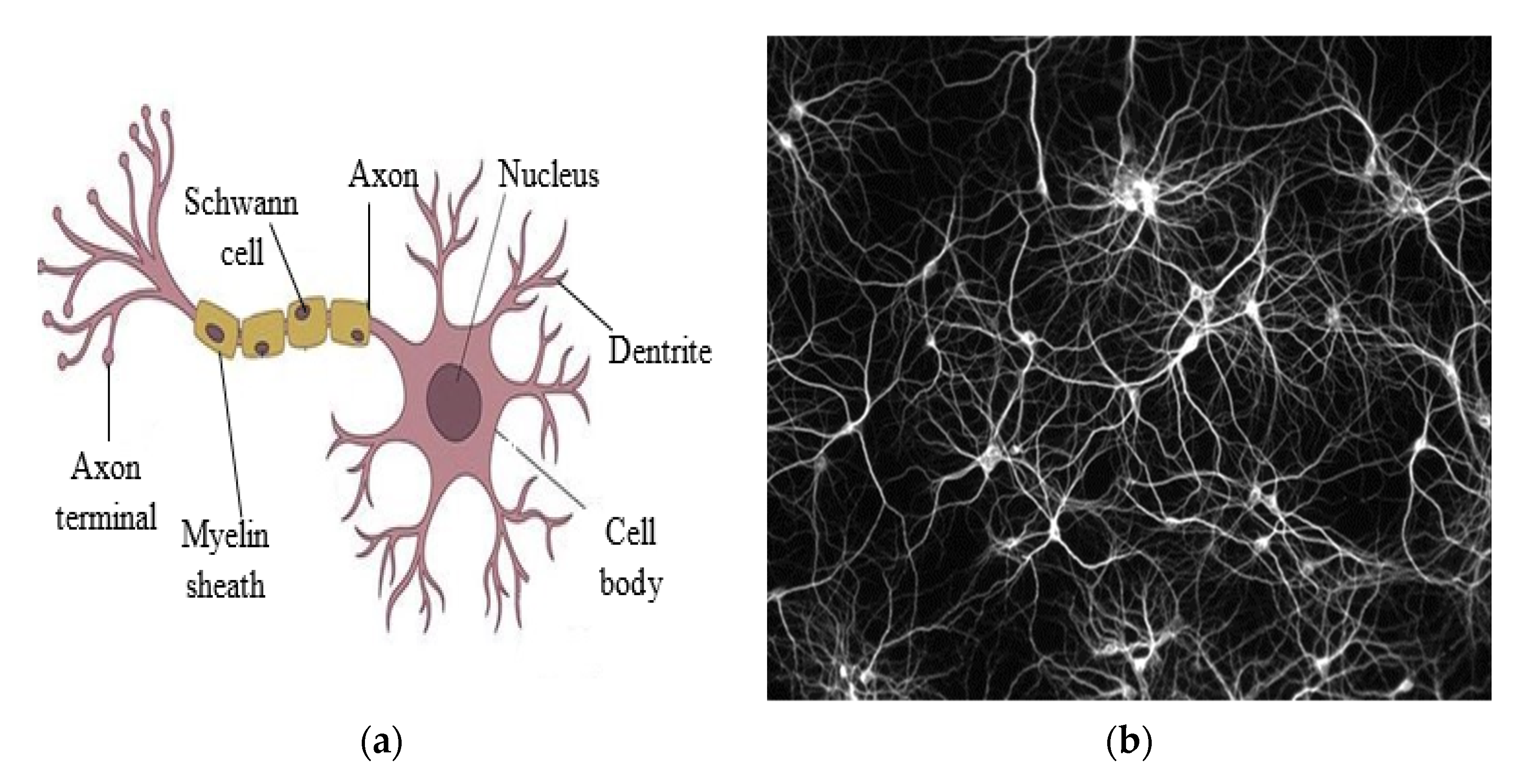
Figure 1. (a,b) Biological Neural Network [10].
Geotechnics 01 00008 g001
Figure 2. Typical Neuron showing Associated Edge Weights.
Geotechnics 01 00008 g002
Figure 3. A Typical ANN Architecture Showing Neurons and Layers.
Geotechnics 01 00008 g003
Figure 4. (a) Recurring Network; (b) Feed Forward Network.
Geotechnics 01 00008 g004
Figure 5. Experimental versus ANN-Predicted UCS values [50].
Geotechnics 01 00008 g005
Figure 6. The selection of optimum number of neurons in hidden layer [52].
Geotechnics 01 00008 g006
Figure 7. Observed Versus Predicted UCS [52].
Geotechnics 01 00008 g007
Figure 8. The selection of the optimum number of neurons in hidden layer [55].
Geotechnics 01 00008 g008
Figure 9. Predicted and experimental observations [56].
Geotechnics 01 00008 g009
Figure 10. Mean square error versus number of neurons in the hidden layer [63].
Geotechnics 01 00008 g010
Figure 11. The experimental and predicted resilient modulus [65].
Geotechnics 01 00008 g011
Table 1. Statistical Evaluation of the Performance of ANN and MVR models [50].
ModelDatasetStatistical Parameter
R2MSEMAE (%)
ANNTraining data0.9920.343.65
Testing data0.9641.508.34
MVRTraining data0.8287.2419.20
Testing data0.8088.0419.26
Table 2. Classification of shrink-swell clays [51].
Modified Plasticity Index I P Volume Change Potential (VCP)
>60Very high
40–60High
20–40Medium
<20Low
Table 3. Statistical evaluation of the performance of ANN and MVR models [55].
ModelDatasetStatistical Parameter
R2MSERSME
ANNTraining data0.98130.03950.1987
Testing data0.971451.347.1651
MVR 0.887068.76038.2921
Table 4. ANN performance using various training algorithms [60].
Training AlgorithmRMSE
Conscience bias learning function0.76937.08
Gradient descent weight and bias learning function0.89913.98
Gradient descent with momentum weight0.91636.66
Levenberg–Marquardt function0.943170.49
Hebb weight learning rule0.87612.4
Table 5. ANN performance using various training algorithms [61].
Training AlgorithmRMSE
Quasi-Newton back propagation0.887121.083 × 10−4
Bayesian regularisation back propagation0.851904.983 × 10−5
Conjugate gradient back propagation with Powell–Beale restarts0.941223.776 × 10−7
Conjugate gradient back propagation with Fletcher–Reeves updates0.811677.339 × 10−6
Conjugate gradient back propagation with Polak–Ribiére updates0.858192.964 × 10−9
Gradient descent back propagation0.948629.985 × 10−9
Levenberg–Marquardt back propagation0.986958.0242 × 10−11
One-step secant back propagation0.923351.388 × 1010
Scaled conjugate gradient back propagation0.969041.946 × 10−6
Table 6. Details of ANN Models and Performance.
ANN DataNetwork ArchitectureModel PerformanceReferences
Soil Parameter InvestigatedANN Input VariablesNo. of Data UsedNo. of Training Data UsedNo. of Testing Data UsedNo. of Validation DataNo. of Hidden LayersNo. of Neurons in Hidden LayerTraining Algorithm UtilisedTrainingValidationTesting
UCS8 Inputs. LL, PI, GGBS content, PFA content, Molarity, activator/binder ratio, Na/Al ratio, Si/Al ratio28370%15%15%19Bayesian regularizationR = 0.996, MSE = 0.34, MAPE (%) = 3.65 R = 0.982, MSE = 1.50, MAPE (%) = 8.34[50]
UCS (7 days)Gs, LS, CU, CC, LL, PL, OMC, MDD7270%15%15%111-R = 0.9782R = 0.996R = 0.9711[52]
UCS (14 days)Gs, LS, CU, CC, LL, PL, OMC, MDD7270%15%15%111-R = 0.9824R = 0.9843R = 0.9615[52]
UCS (28 days)Gs, LS, CU, CC, LL, PL, OMC, MDD7270%15%15%111-R = 0.9946R = 0.9992R = 0.9929[52]
UCSPercentage of Clay, percentage of RHA, percentage of cement, percentage of PFA, curing duration(days)12970%15%15%110Levenberg–MarquardtR2 = 0.9813, MSE = 0.0395, RMSE = 0.1987 R2 = 0.9714, MSE = 51.34, RMSE = 7.1651[55]
UCSCuring duration, compaction energy.8070%15%15%28 in each layer R2 = 0.924R2 = 0.908R2 = 0.889[56]
UCSST, MC, We, CM, DI, L, CA, SV, D, MS, DS, CD, curing time (days), CT21680%20% 150AdamR = 0.980 (Average), MAE = 115.29, RMSE = 231.2 R = 0.925 (Average), MAE = 292.2, RMSE = 419.82[57]
UCSMoisture content, cement (percentage), air foam(percentage) and waste fishing net content (percentage)5170%30% 212 and 10 neuronsLevenberg–MarquardtR = 0.95, MAE = 3.9001, RMSE = 9.1948 R = 0.94, MAE = 8.6535, RMSE = 10.3390[58]
CBR (28 days)LL, PL, OMC and MDD4970%30%---Differential evolutionR = 0.98 R= 0.86[59]
CBR (28 days)LL, PL, OMC and MDD4970%30%---Levenberg–MarquardtR = 0.96 R= 0.93[59]
CBR (28 days)LL, PL, OMC and MDD4970%30%---Bayesian regularizationR = 0.96 R= 0.93[59]
CBRType of ash, mix proportion (percentage), LL, PL, MDD, OMC and number of geogrid layers210---17Levenberg–MarquardtR = 0.94472R = 0.93327R = 0.94685[60]
CBR (28 days Soaked)LL, PI, percentage of PFA, OMC, MDD and no. of geotextile layers----1-Levenberg–MarquardtR = 0.99846R = 0.98508R = 0.92149[61]
CBR (28 days Soaked)Percentage of RHA, percentage of lime, curing time (days), OMC and MDD4870%15%15%112-R = 0.9948R = 0.98909R = 0.98895[62]
CBR (Soaked)PL, LL, GS, LS, CU, CC, OMC and MDD7270%15%15%18-R = 0.9988R = 0.9996R = 0.9976[63]
CBR (Unsoaked)PL, LL, GS, LS, CU, CC, OMC and MDD7270%15%15%117-R = 0.9912R = 0.9993R = 0.9806[63]
Coefficient of permeability (K)percentage passing 0.005 mm, PI, MDD, lime percentage, pozzolan percentage, Cd6970%15%15%19 R = 0.9968R = 0.98883R = 0.99405[64]
Resilient Modulus (Mr)Percentage of cement, percentage of lime, PI, percentage of silt, percentage of PFA, OMC, MC and clay125---19-R = 0.9517-R = 0.9467[65]
MDDLL, PI, LS, clay-silt ratio, sand content, lime content, cement content, asphalt content in percentage19252%24%24%118Gradient descent momentumR2 = 0.9183, MSE = 0.28%, MAE = 4.44% R2 = 0.9101, MSE = 0.26%, MAE = 4.24%[66]
OMCLL, PI, LS, clay-silt ratio, sand content, lime content, cement content, asphalt content in percentage19252%24%24%115Gradient descent momentumR2 = 0.9025, MSE = 88.21%, MAE = 118.37% R2 = 0.8916, MSE = 89.57%, MAE = 113.03%[66]
MDDGS, LS, free swell, D10, D30, D60, CU, CC, LL, PL9070%15%15%17 R = 0.9946R = 0.9715R = 0.9754[67]
OMCGS, LS, free swell, D10, D30, D60, CU, CC, LL, PL9070%15%15%15-R = 0.9977R = 0.9779R = 0.8855[67]
- Not reported.
Table 7. The number of datasets utilised for model development.
Network Architecture ANN Data References
No of Hidden LayersNo of Neurons in Hidden LayerANN Input VariablesNo. of Network ParametersNo. of Data UsedNo. of Training Data UsedRemarks
19891283198Sufficient[50]
11181117250May overfit[52]
11057112990Sufficient[55]
28 in each layer21058056May overfit[56]
15014801216172May overfit[57]
212 and 1042015136May overfit[58]
--4-4934No Remark[59]
177-210-No Remark[60]
1-6---No Remark[61]
1125854834May overfit[62]
188817250May overfit[63]
11781717250May overfit[63]
196736948May overfit[64]
198-125-No Remark[65]
1188181192100May overfit[66]
1158151192100May overfit[66]
1710859063May overfit[67]
1510619063Sufficient[67]
- Not reported.
Publisher’s Note: MDPI stays neutral with regard to jurisdictional claims in published maps and institutional affiliations.