Article

WeedNet-ViT: A Vision Transformer Approach for Robust Weed Classification in Smart Farming

Department of Natural, Engineering and Technology Sciences, Faculty of Graduate Studies, Arab American University, Ramallah P.O. Box 240, Palestine
*
Author to whom correspondence should be addressed.
Geographies 2025, 5(4), 64; https://doi.org/10.3390/geographies5040064 (registering DOI)
Submission received: 12 September 2025 / Revised: 10 October 2025 / Accepted: 15 October 2025 / Published: 1 November 2025

Abstract

Weeds continue to pose a serious challenge to agriculture, reducing both the productivity and quality of crops. In this paper, we explore how modern deep learning, specifically Vision Transformers (ViTs), can help address this issue through fast and accurate weed classification. We developed a transformer-based model trained on the DeepWeeds dataset, which contains images of nine different weed species collected under various environmental conditions, such as changes in lighting and weather. By leveraging the ViT architecture, the model is able to capture complex patterns and spatial details in high-resolution images, leading to improved prediction accuracy. We also examined the effects of model optimization techniques, including fine-tuning and the use of pre-trained weights, along with different strategies for handling class imbalance. While traditional oversampling actually hurt performance, dropping accuracy to 94%, using class weights alongside strong data augmentation boosted accuracy to 96.9%. Overall, our ViT model outperformed standard Convolutional Neural Networks, achieving 96.9% accuracy on the held-out test set. Attention-based saliency maps were inspected to confirm that predictions were driven by weed regions, and model consistency under location shift and capture perturbations was assessed using the diverse acquisition sites in DeepWeeds. These findings show that with the right combination of model architecture and training strategies, Vision Transformers can offer a powerful solution for smarter weed detection and more efficient farming practices.

1. Introduction

Weeds directly affect the productivity of agricultural crops by competing for natural resources such as water, light, and nutrients. This is why they are considered one of the most prominent challenges facing agriculture around the world [1]. Detecting weeds in crops is extremely difficult, due to the great similarity in the colors of weeds and crops, as well as the possibility of similar texture, color, or shape. Identifying weed species is also important for applying control methods such as herbicides [2]. In the past, to control weeds, farmers relied on manual methods and chemical pesticides, but these methods are often harmful to the environment and the people who are exposed to them are expensive, and are not sustainable. For example, chemical pesticides can contaminate water and soil and, over time, contribute to the development of weed resistance to pesticides [3,4]. For all these reasons, there is an urgent need to adopt smart and effective techniques to identify weeds and manage them sustainably.
With the emergence of deep learning technologies, digital image processing, and vision transformers, recent years have witnessed remarkable progress in the application of artificial intelligence in smart agriculture [5]. Among these techniques, convolutional neural networks (CNNs) have been widely used for weed detection and classification with high accuracy [6]. However, high-performance neural networks often depend on the design of specialized structures and may have difficulty handling data with complex and variable patterns such as those generated by weeds under diverse environmental conditions and also in the diversity of backgrounds in weed images [7]. Hence, the need for transformer technology as a powerful and effective tool for processing complex data has become important.
Transformer technology emerged as a powerful and effective tool in processing complex data. The use of transformers in computer vision, through models such as Vision Transformer (ViT), has proven effective in dealing with high-resolution images, although it was originally designed to process textual data [8]. This approach has the ability to analyze spatial features and global relationships within images, making it suitable for weed classification in agricultural settings [9]. In addition, images captured by ground cameras or drones are an important source of data in smart agriculture. This technology allows for the collection of high-quality data on a large scale, which helps improve the accuracy of AI-based models [10]. Combining transformer-based models with large-scale agricultural imagery can significantly improve automated weed management.
Despite this progress, challenges remain. Deep learning models for weed classification still require interpretability mechanisms to explain their decisions, and the effectiveness of vision transformers in this domain remains insufficiently explored. Weed/crop vision models still require interpretability to explain decisions in field contexts, and the role of Vision Transformers in weed detection/classification is comparatively underexplored relative to CNNs (see, e.g., [1,2,11,12]). Accordingly, the aims of this work were as follows: (i) to evaluate a ViT model against strong CNN baselines on DeepWeeds; (ii) to quantify the effect of data-imbalance strategies (class weighting vs. oversampling) on accuracy; (iii) to provide initial interpretability via attention-based saliency inspection; and (iv) to assess consistency under location shift and capture perturbations using the multi-site, variable-condition imagery in DeepWeeds.

2. Literature Review

The field of weed classification using artificial intelligence has received the attention of researchers, as much of their research has focused on improving the accuracy and performance of models using different techniques. In this section, we discuss the most prominent research conducted in this field, highlighting its results, the challenges it faced, and the positives outcomes that were achieved. As reported in [13], machine-learning methods such as Random Forest (RF), Support Vector Machine (SVM), and CNN achieved ~85–99% accuracy in plant disease classification applications, and UAV imagery was also used to classify crops and weeds. A wide range of studies have focused on CNN-based weed classification. For example, accuracy above 85% was reported in [14], and a CNN model for real-time semantic segmentation improved performance by up to ~13% when leveraging background knowledge [6]. The researchers presented this study [15] on the “DeepWeeds” dataset, which contains 17,509 images classified into 9 types of weeds in Australia. The researchers used the deep learning models Inception-v3, which achieved an accuracy of 95.1%, and ResNet-50, which achieved a classification accuracy of 95.7%. Other studies [15,16] reviewed recent research on the application of drones using convolutional neural networks (CNNs) and computer vision techniques to weed detection.
In 2024, a team of researchers developed artificial intelligence techniques to distinguish weeds with higher accuracy using imaging data, as studies showed that using advanced image analysis algorithms helped classify weeds more accurately and at a lower cost compared to traditional methods, The researchers in [17] used ViT model to classify plant diseases. They showed that combining ViT with a CNN architecture maintained inference speed without sacrificing accuracy and the accuracy was between 96% and 98%. The researchers in [18] proposed an advanced application of ViT on Unmanned Aerial Vehicle (UAV) images to classify crops such as beetroot, parsley, and spinach. This model outperformed state-of-the-art CNN models using a relatively small dataset. Studies [11,12] were on the application of visual transformers to classify weeds and crops. They focused on taking advantage of the self-attention mechanism that characterizes transformers to facilitate the processing of complex spatial and spectral patterns in agricultural fields. Their results showed a clear improvement in accuracy compared to traditional CNNs, with some models achieving 94% accuracy. But they faced challenges related to the need for labeled data to train models.
These studies [16,19] presented a comprehensive study of the integration of image processing techniques with intelligent systems, focusing on the stages of image processing and enhancement, feature extraction and classification for pest detection, and increasing the accuracy of image processing techniques used in agricultural applications. However, challenges included variable lighting, complex backgrounds, overlap between weeds and target plants, and the impact of environmental changes on the accuracy of models. Also, this study [17] conducted a comprehensive study of deep learning at the agricultural level in all its forms and found that plant stress monitoring and classification applications using CNN, ViT, transfer learning and few-sample decomposition (FSL) techniques achieved significant improvements in accuracy. Other studies [8] presented a ViT model based on image segmentation and applied a self-attention mechanism instead of convolutional layers. This model outperformed traditional networks in terms of performance and accuracy, reaching 88.55% using ViT-B/16.
On the other hand, the researchers also worked on integrating image pre-processing techniques with deep learning to improve performance. For example, studies such as [20] used segmentation techniques to improve crop and weed separation, which helped reduce classification errors by up to 15%. Given the challenges common to these studies, several key points emerge among them: Environmental changes, as most studies have confirmed that lighting, shade, and soil types greatly affect the quality of images and the accuracy of classification; a lack of diverse data, since the need for training data that includes different environmental conditions and patterns has been a common problem, which increases the risk of bias in the models; and implementation costs, as the use of advanced devices such as drones or multispectral cameras is challenging in terms of cost, making the application of these technologies limited in some regions [21]. The researchers in [22] reviewed the advanced capabilities of agricultural robots, and the results showed that the integration of vision and sensing systems with artificial intelligence improved the accuracy of classification processes by a percentage ranging between 85% and 95%. The researcher in [23] presented and discussed remote sensing techniques, satellite data, and drones, and confirmed that Normalized Difference Vegetation Index (NDVI) and Enhanced Vegetation Index (EVI) vegetation indices are widely used in productivity estimation and early disease detection, and the prediction accuracy exceeded 90% in some studies. The authors in [18] combined Explainable AI Techniques with deep learning to improve visual detection of wheat diseases. Two other studies [17,24] used Vision Transformers models after converting audio signals into spectrograms, due to the flexibility of these models in handling different data and the ability to enhance them with interpretation techniques to understand the model’s decisions. Transformers models are not only used in traditional computer vision but are also effective in classification tasks.
These studies [22,23,24] talked about hybrid models that combine CNNs and transformers to improve performance while maintaining efficiency. They highlighted that combining feature extraction capabilities in convolutional networks and attention mechanisms in transformers led to improving the accuracy of weed detection by a rate ranging between 7% and 10% compared to using CNNs. The results were positive, but these models suffered from additional complexity in structure and increased training time. This study [25] developed a hybrid multi-class leaf disease identification model combining Variational Autoencoder (VAE) and ViT and achieved an accuracy of 93.2%.
Overall, previous studies have made significant contributions to improving weed classification accuracy but have demonstrated the need for innovative solutions to overcome these challenges.
Although there has been significant progress in the use of deep learning techniques and weed classification as addressed in previous studies, there are some challenges and gaps that still exist, such as the limited environmental diversity of data: most studies have relied on environmentally limited datasets, which reduces the ability of models to generalize under variable environmental conditions (e.g., light, shade, and different soil types), Another issue is the heavy reliance on huge data for training: the models used require large amounts of high-quality data, which poses a challenge in cases where data is limited. Also, there are high computational costs: modern models such as Transformers provide outstanding performance but depend on high computational resources, which reduces their usefulness in field applications. Finally, there is a lack of real-life experience, as much research has focused on laboratory or simulated environments and has not been adequately tested in real agricultural field conditions. This study aims to address some of these gaps by developing advanced classification model based on Transformers technology, with targeted improvements to handle data in unbalanced categories by comparing the application of data augmentation techniques and class weighting technology. This study introduces a framework to solve the problem of data imbalance and rely on fewer computing resources without sacrificing accuracy. The models are also tested in real-world environments with varying environmental conditions, allowing for generalization of the models and a practical and realistic evaluation of their efficiency.
Thus, the study seeks to present a new model that balances high performance with practical applicability, which contributes to supporting smart agriculture and reducing reliance on traditional methods of weed control. The remainder of this paper is divided into several main sections, with Section 3 examining the proposed methodology in detail. This is followed by Section 4, which reviews the experiments, results and discussion of the findings, and Section 5 concludes the paper by reviewing the main conclusions, while providing valuable recommendations for possible future work.

3. Materials and Methods

Weeds are a constant threat to agriculture, causing crop losses due to their similarity to beneficial crops. Therefore, there is a need for technical solutions that contribute to their classification and accurate differentiation. In this section, a classification model was built that can recognize weed species from images of their leaves through a series of steps. This work was implemented using the PyTorch 2.3.1 library and Python 3.10.13 (CUDA 12.1, cuDNN 9.1). We conducted a series of experiments using an NVIDIA GeForce GTX 950M graphics card and 12 GB of DDR4 RAM at 2400 MHz, and it is acknowledged that this legacy GPU constrains batch size and throughput; conclusions are expected to transfer, but scalability on contemporary accelerators (e.g., RTX/A-series) should be verified. The process also involved pre-processing steps, a data augmentation technique and adjusting the same training parameters, including learning rate, batch size, and number of epochs. All experiments were performed on the DeepWeeds dataset, which consists of 17,509 labeled images. The work also involved selecting the appropriate model, and finally applying training, interpretation, and evaluation strategies to achieve accuracy in classifying weed species. For interpretability, transformer attention maps (attention rollout) were generated and inspected to verify that high-importance regions aligned with weed structures; no additional figures were required. This is to ensure the reliability of the results and to ensure that the model works effectively and can be generalized to new, previously unseen data, as shown in Figure 1. To contextualize scalability, we report per-epoch time, peak VRAM at batch 32, and single-image inference latency for ViT vs. lightweight CNNs.

3.1. Dataset Description

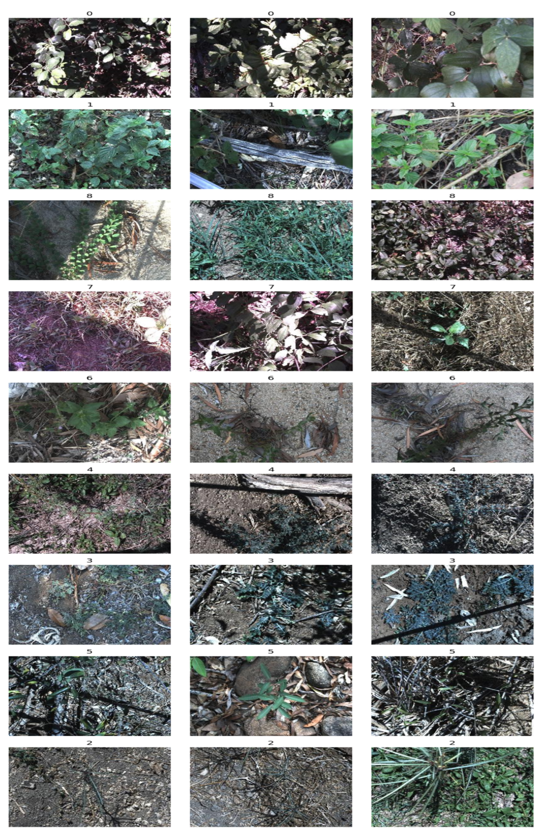
The dataset of this research work included 17,509 images of 256 × 256 pixel size in color, representing 9 different weed species classes namely Chinee Apple, Lantana, Parkinsonia, Parthenium, Prickly Acacia, Rubber Vine, Siam Weed, Snake Weed, In addition to a negative category, which represents images free of weeds [11]. This dataset was specifically designed for weed species classification, which was mainly collected from grassland environments using an integrated imaging system operating under natural agricultural conditions in Northern Australia, reflecting a real diversity of backgrounds, shooting angles, lighting, and climatic conditions. The images were captured across eight distinct locations in Queensland, including Black River, Charters Towers, Culloden, Douglas, Hervey Range, Kelso, McKinley and Paloma. The images are organized into folders by category name, along with descriptive information including weather data, GPS coordinates, and date, enabling researchers to perform spatial analysis or environmental modeling. Figure 2 shows a sample of the dataset containing 3 random images from each of the 9 categories.
What also distinguishes this collection is that it was taken in agricultural locations with significant variation in environmental factors, including weed density, shade, terrain, and background. This metadata accompanying the images, such as geographic location (GPS), weather conditions, and time, this allows for expanded analysis of the spatial distribution of weeds as well as environmental monitoring. All nomenclature files consist of comma-separated values (CSVs) that describe the nomenclature and types. DeepWeeds is an ideal database for evaluating modern deep learning models such as vision transformers, as it provides real-world challenges that mimic practical applications in agricultural fields. Table 1 shows the classes of weed images in the dataset used in the proposed approach.

3.2. Data Preparation and Preprocessing

3.2.1. Addressing Class Imbalance in Data

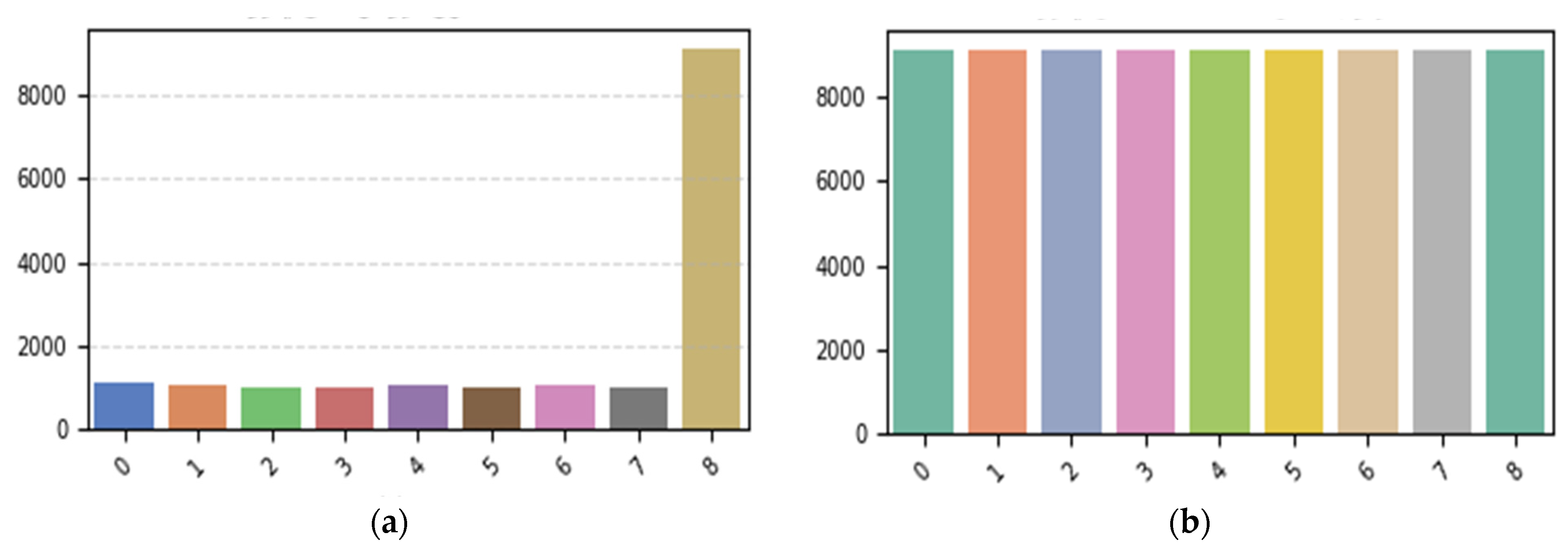
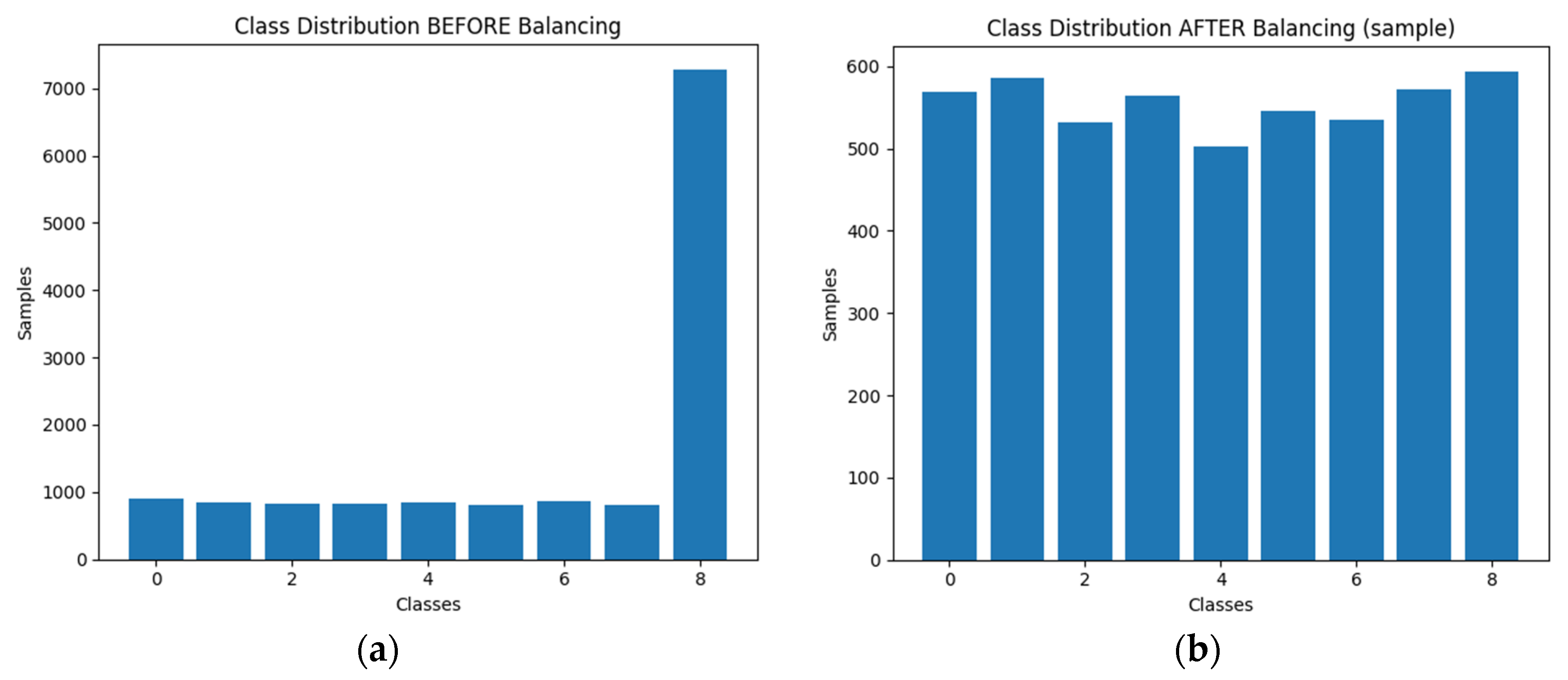
The DeepWeeds dataset proposed for this work, which includes 17,509 images distributed across nine categories, shows an uneven distribution of images across categories. Figure 3a shows that the “Negative” category—which includes images free of weeds—contains a much larger number of samples compared to the number of samples in the other eight categories, which include different types of weeds. This imbalance in the images has led to a noticeable class imbalance, which causes the model to be biased towards this larger class during the training process. This difference in the number of images led to an imbalance between the classes, causing the model to bias toward the more represented class during training. To address this issue, certain measures were taken, such as: Using a weighted cross-entropy loss function, which gives greater weight to classes with fewer images, reducing the model’s bias toward the class with the largest number of images. The weights were calculated based on the relative distribution of each class. Data augmentation techniques such as lighting changes, rotation, blurring, and random cropping were also applied to images of underrepresented classes to increase their size without compromising visual meaning, ensuring that the model works accurately and is able to distinguish between the classes without bias in the training data. Concretely, we used PyTorch’s CrossEntropyLoss with a per-class weight vector that is inversely proportional to each class’s frequency in the current training split; the weights were then scaled so that their average equals 1, placed in label-index order (Negative, Chinee Apple, Lantana, Parkinsonia, Parthenium, Prickly Acacia, Rubber Vine, Siam Weed, Snake Weed), moved to the GPU as a float tensor, and recomputed for every fold/split. For oversampling runs, we employed WeightedRandomSampler with sampling probabilities proportional to these weights. Because DeepWeeds spans eight capture locations and diverse lighting/backgrounds, splits were prepared to preserve this diversity so that consistency under location shift and capture perturbations could be observed. Figure 3b shows the data after balancing using the oversampling technique. Figure 4a shows the data before balancing, and Figure 4b shows another technique for balancing the data, which is by weighting the categories, where greater weight is given to rare categories.

3.2.2. Preprocessing and Augmentation

We prepared the data to be entered into the model by preparing the images through the following steps: Data cleaning: Damaged images containing noise and quality issues were excluded. Resizing: All images were resized to a uniform size of 256 × 256 pixels to match the input dimensions of the ViT model. Pixel values were normalized to a range of 0 to 1 by dividing the pixel values by 255. Data augmentation: To improve generalizability and avoid overfitting, data augmentation techniques were applied to help the model learn more robust features, such as random rotation up to 20 degrees, random horizontal shifting, random augmentation, zooming, cropping, and lighting changes. Color enhancements were also implemented to address challenges that may arise due to environmental changes such as shadows or bright lighting. In addition, an oversampling technique has been used to increase the representation of less frequent classes in the data, contributing to a better balance between different classes and reducing the model’s bias towards more represented classes. The dataset is then divided: The dataset was divided into training (60%), validation (20%), and testing (20%) sets. This division was performed according to the division specified in the labels.csv file to ensure that there was no overlap between groups [15]. The proposed model was trained and validated on each of these splits, allowing for a thorough analysis of its robustness and learning behavior under different data configurations. This partitioning ensures that the model is trained and evaluated on separate, non-overlapping subsets of the dataset, allowing for a robust evaluation of performance.
The experiments were conducted in two stages. The first stage relied on evaluating a set of lightweight CNN models using cross-validation to measure accuracy, and the second stage was to evaluate the ViT model and compare it with previous models. A set of statistical metrics used in classification systems and model evaluation were adopted, including accuracy, precision, recall, F1 score, and area under the ROC curve. In addition, ROC curves and classification reports were used to evaluate the performance of the models and their ability to discriminate.
Different CNN models were tested, and the lightweight models MobileNet V2, ConvNeXt-Tiny, ShuffleNet V2, EfficientNet B0, RegNet_X_400MF, and ResNet-18 were selected. They were trained using k-fold cross-validation to reduce bias. All models were subjected to the same preprocessing settings, data augmentation techniques, and training parameters, such as learning rate, number of epochs, and batch size, to achieve a fair comparison. A set of statistical measures used in classification systems were adopted to evaluate the performance of models, such as accuracy, precision, recall, F1 coefficient, and area under the ROC curve. ROC curves were also used to estimate the discriminatory ability of models, and training/validation curves (accuracy/loss curves) were used to understand the behavior of the model during learning.
Various strategies were also applied to address the imbalance of the DeepWeeds dataset, in order to obtain better classification model performance and improve classification. Initially, a technique of giving higher weights to underrepresented classes was used, which demonstrated the model’s ability to achieve outstanding performance. Oversampling was also applied to underrepresented classes, which led to a decrease in training accuracy. However, this strategy reduced the problem of overfitting.

3.3. Classification Method

3.3.1. CNN Models

Convolutional networks were introduced [26] and later became one of the cornerstones in the field of computer vision. Figure 5 below shows the overall CNN architecture with a brief explanation of each of the models used in this research. These models are distinguished by their ability to achieve high-accuracy results in image classification and recognition.
CNN processes weed images through convolutional operations; features are mapped to extract important semantics while preserving spatial relationships. The basic architecture of a CNN consists of convolutional layers that apply filters to learn patterns, pooling layers to reduce the dimensionality of feature maps, and final classification in fully connected layers. The CNN model architecture begins with an input layer designed for 200 × 200 × 3 RGB images. This is followed by three convolutional layers containing 32, 64, and 64 filters, each with a kernel size of 3 × 3. This is repeated across all convolutional layers to preserve spatial dimensions. ReLU activation is propagated through each layer to accommodate diverse models in capturing complex patterns. This is followed by batch normalization to stabilize the learning process and improve generalization. The outputs from the intermediate layers are normalized, which speeds up training. Sometimes, max pooling is applied in the batch normalization layer with a pooling size of 2 × 2 to reduce the dimensions of feature maps and reduce computational complexity.
EfficientNet is a model characterized by its high efficiency in performance with a smaller number of operations compared to other models. EfficientNet-B0 to B7 is one of the most popular versions, as it achieves outstanding performance in classification with less resource consumption, which makes it ideal for training on devices with limited capabilities.
MobileNet is a convolutional neural network designed for high efficiency and particularly light weight, making it suitable for applications that require limited resources. Developed by Andrew Howard, it delivers outstanding performance in deep neural networks on embedded devices such as low-power devices and smartphones as it can meet the needs of devices with limited capacity [26].
DenseNet is one of the prominent architectures of CNN, where each layer in the network is connected to all subsequent layers. Unlike traditional architectures that rely only on the last layer for decision making, DenseNet uses all layers to contribute to the classification process, enhancing the flow of information within the network. Connections between layers close to the input are reduced, while layers closer to the output play a role in improving training accuracy. The design of DenseNet121 is based on the use of feedforward connections between each layer and all subsequent layers, ensuring that shorter connections are exploited for feature propagation and reducing the number of parameters while improving network efficiency. DenseNet121 is one of the major versions of DenseNet, along with others such as DenseNet169, DenseNet201, and DenseNet264 [27].
ResNet-50 is a CNN architecture based on deep learning and residual network techniques. It was developed by the Microsoft team and was one of the best performing algorithms in computer vision of 2015. ResNet-50 consists of 50 deep layers and more than 25.6 million parameters. The network is based on the concept of residual blocks, where a convolution is combined with the identity block. The inputs remain equal to the outputs in this design, and the final layer is represented by a fully connected layer, the raw signal or input (x) is matched with the identity (ID) mapping in each block. Thus, the residual signal of each block is calculated as the product of the sum of the input and output values, to improve the flow of information through the network and solve the problem of disappearing gradients in deep networks [28].
The ConvNeXt model is a modern extension of convolutional networks, in which the traditional CNN architecture has been redesigned to be more compatible with modern optical transformer architectures. It relies on improvements inspired by ViT, such as large kernel sizes and layer normalization, so it delivers transformer-like performance while maintaining computational efficiency. It combines the power of CNNs with the smoothness of transformers, so it is used in large-scale data classification [29].
RegNet is based on a regularized design that allows for a balanced increase in the number of channels and layers to achieve the best accuracy versus computational cost. It is a network model resulting from design space exploration, developed by finding simple, generalizable design rules. One of its most important features is that it allows the creation of families of networks of different sizes while maintaining training and inference efficiency [30].
ShuffleNet is an ultra-lightweight model designed specifically for mobile devices and limited-capacity environments and is one of the most energy- and memory-efficient models available. The model is based on the Channel Shuffle concept, which enables highly efficient information exchange between channels while reducing the number of computational operations (FLOPs). It also uses group convolutions to reduce complexity without compromising representation quality.

3.3.2. Vision Transformers

To avoid overlap with Section 3.3.1, we summarize only ViT-specific components: patch embedding (16 × 16), a transformer encoder (multi-head self-attention + MLP), and a classification head. ViT’s global self-attention models long-range spatial relations that CNNs capture indirectly, which we hypothesize benefits weed/crop separation under varied backgrounds and lighting [8,31]. The ViT model revolutionized the field of computer vision by incorporating transformation principles developed for natural language processing. The model processes images into patches to preserve them well. Vision Transformers use sequential processing to handle image data, which is an essential factor when working on more complex visual abstractions. Moreover, its unique design allows parallel processing, which leads to accelerated training time. Due to its design, the self-attention mechanism can handle connections across the entire input range, making it more effective compared to CNN models [31]. As it takes advantage of the strengths of the transformer in image classification, which makes it easy to implement and enhances the model’s ability to classify weeds with high accuracy, compared to traditional models such as CNN.
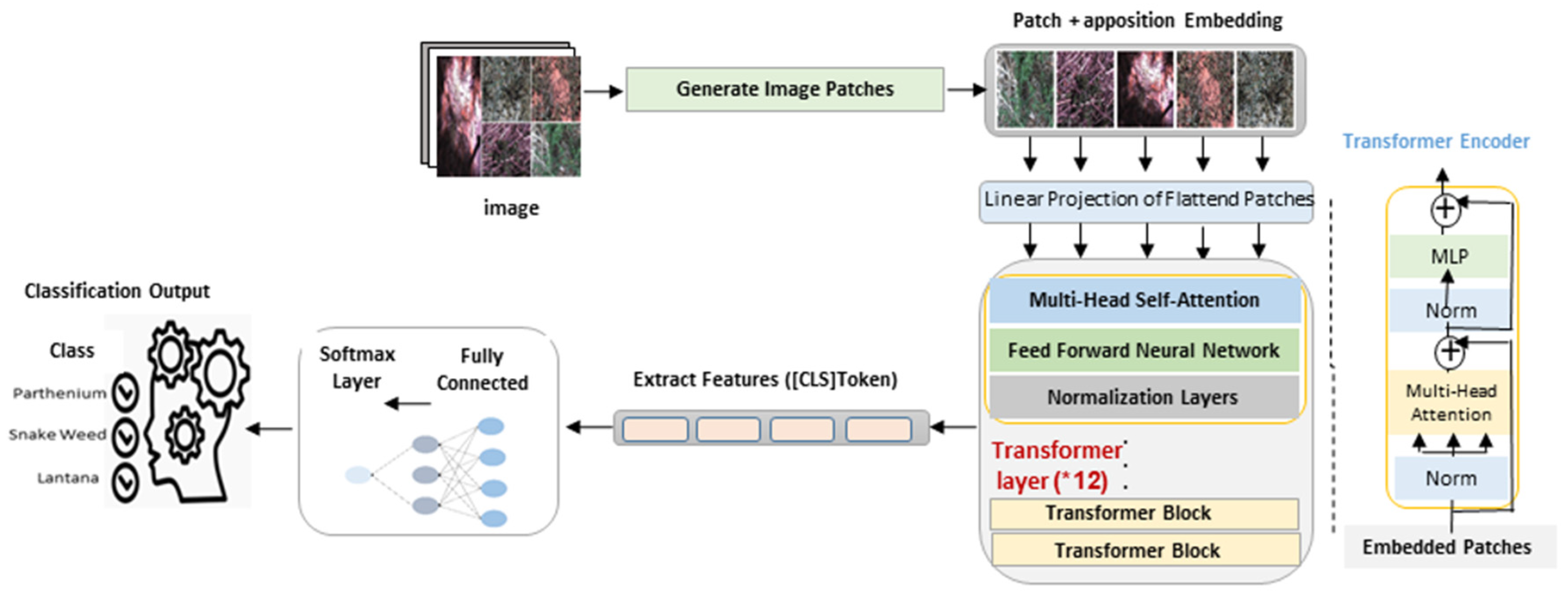
Images are converted into vector representations using vision transformer frameworks, an architecture based on multi-head self-attention mechanism and feed-forward neural networks. This arrangement allows the model to recognize advanced spatial patterns and deep representations of images, and to understand image context and long-term dependencies. Patch sequences include a unique pre-added class code that collects data from all patches and is fed into the output classification module. Patch operations include embedding positions to preserve spatial information. The following Figure 6 shows the vision transformer structure. First, the image is divided into a number of patches with a length of 16 × 16 pixels. These patches are then flattened and linked to a vector, which is used to feed the transformer with input codes, and the classification head in the transformer encoder makes predictions.
The transformer layers are configured to allow the model to process images non-sequentially, so that it can extract fine spatial features. And use a set of optimal parameters such as the number of attention peaks and the number of layers to achieve optimal performance [32]. The ViT architecture used consists of the following:
  • Patch embedding: The images are divided into 16 × 16 patches. Each piece is rectified into a vector and then embedded into a higher dimensional space by a learnable embedding layer.
  • Transformer encoder: It consists of multi-head self-attention and feed-forward neural networks, and here the combined patches are passed through the transformer encoder layers. The encoder can capture the relationships between different parts of the image.
  • Classification Head: The output of the transformer encoder is passed through the classification head, which consists of a fully connected layer (Dense) followed by a Softmax activation function to produce the final probabilities of the types.
  • Hyperparameters: The following hyperparameters were used during training: Learning rate, Batch size to capture enough data at each training step, Loss function, Number of Epochs, CrossEntropyLoss was used in multi-class classification due to its effectiveness, Optimizer AdamW was to handle weight erosion, and OneCycleLR was used to adjust the learning rate adjusted dynamically during training to prevent the model from falling into local minima. A normalized L2 weight decay was used to avoid overfitting and ensure the generalizability of the new data.
We used the ViT-base-patch16-224 model with fine-Tuning to adapt the model to the task of weed classification. We used Hugging Face’s Transformers library and the PyTorch library for training and assessment. The ViT-Base Patch16 224 model, available in the timm library, is designed to process 224 × 224 pixel images by splitting them into 16 × 16 pixel patches. He performed well in weed classification, object detection and semantic hashing tasks, and demonstrated superiority over traditional CNNs when trained on large datasets. It has scalability and leverages big data and computational resources to improve performance. Vision Transformer’s self-attention mechanism is more effective at capturing the overall context of an image than the local convolutions used in CNNs, so it is characterized by adapting to different computer vision tasks with minor modifications. In the task of weed classification, the ViT model was used to extract accurate patterns in plant images, allowing harmful and harmless species to be identified with high accuracy. Instead of relying on traditional image characteristics such as colors and borders, it creates a semantic space that can recognize more complex patterns in image data, enhancing classification accuracy, shown in Table 2.
We will explain the training procedures and evaluation metrics used in the proposed vision transformer model for weed classification. The data was divided into training and test sets using cross-validation to ensure that overfitting did not occur. The model was trained using the Adam algorithm with a dynamic learning rate to speed up the training process and reduce the time required. The model was evaluated periodically during the training process using the accuracy index and validation loss, which helps in constantly adjusting the parameters, and the best model was saved based on validation accuracy [33] and hyperparameters such those in Table 3.
After training was completed, the model was tested using a separate test dataset that was not used in the training phase. We conducted a comprehensive analysis using a set of indicators to evaluate the efficiency and effectiveness of the model applied to the weed dataset, and in this research, we relied on key performance metrics such as confusion matrix, precision, recall, precision, in addition to the F1 score, as described below (1).
A c c u r a c y = T r u e   P o s i t i v e + T r u e   N e g a t i v e T r u e   P o s i t i v e + T r u e   N e g a t i v e + F a l s e   P o s i t i v e + F a l s e   N e g a t i v e
The number of correct positive categories that are classified is referred to as true positive, while the number of negative categories that are correctly classified is referred to as true negative. Negative categories that are incorrectly classified as positives are known as false positives, while positive categories that are incorrectly classified as negatives are known as false negatives. The proportion of samples that were correctly classified as positive out of the total samples that were assumed to be positive is known as accuracy [34]. This ratio is expressed mathematically using the following equation.
R e c a l l = T r u e   P o s i t i v e T r u e   P o s i t i v e + F a l s e   N e g a t i v e
The percentage of all positive samples that are accurately predicted as positive is called “recall” Recall is calculated according to the following Equation (3).
P r e c i s i o n = T r u e   P o s i t i v e T r u e   P o s i t i v e + F a l s e   P o s i t i v e
The cumulative average of both recall and precision is known as the F1 score and is calculated using the following Equation (4).
F 1 = 2 × P r e c i s i o n × R e c a l l P r e c i s i o n + R e c a l l
Confusion matrix: allows analysis of type I and type II errors. It is used to evaluate the accuracy of classification by giving more detail and provides a comparison of results with traditional models such as multi-spectral models supported by images and convolutional neural networks (CNNs) [35].

4. Results

4.1. CNN Models Performance Evaluation

4.1.1. Convergence Behavior of CNN Models Using Accuracy and Loss Curves

CNN model experiments were conducted as shown in Figure 7 below, which shows the accuracy curves for training and validation data using three methods. Figure 7a shows the results before data balancing for the model that achieved the highest accuracy, and Figure 7b shows the results after balancing using the oversampling technique. Figure 7c shows the results after balancing the data using class weighting.
The figure shows stability and steady improvement in accuracy for both the training and validation datasets. The proposed model maintains stability and high accuracy throughout the training period. This demonstrates the effectiveness of batch normalization and learning rate tuning on model performance. The accuracy curves indicate that the training process for almost all models stabilizes as they gradually approach high and stable values after a number of iterations (epochs), demonstrating the effectiveness of fine-tuning strategies and the balance of generalization between training and validation data.
The following Table 4 shows the accuracy for both training and validation data to others CNN models before balancing: EfficientNet B0 training (98.2%) and validation, followed by ConvNeXt-Tiny achieved the highest training (99.4%) and validation (96.6%) accuracy, followed by MobileNetV2 training (97.4%) and validation (94.5%), RegNet_X_400MF training (97.1%) and validation (94.9%), and ResNet18 training (96.2%) and validation (93.1%). ShuffleNetV2 training (93.4%) performed relatively poorly, with a validation accuracy of 91.4. The results in the table also show the effectiveness of fine-tuning strategies and the balance between generalizations.
This was observed when oversampling was applied to underrepresented groups: the accuracy of the training data decreased, but this was accompanied by improved performance in the validation and test data. This suggests that oversampling contributes to reducing the problem of overfitting and enhances generalizability.

4.1.2. Loss Curve Analysis

Figure 8a below shows the training and validation loss curves for the proposed CNN model that achieved the highest CNN accuracy before balancing and shows in Figure 8b the evolution of the loss values during training and validation for the selected models. All models exhibited a gradual decrease in loss until they reached stability. Figure 8c shows that the loss decreased steadily to levels that ensured the results on the training data and the ability to generalize to the validation data after balancing. EfficientNet B0 achieved the lowest loss, outperforming other models such as ResNet18 and MobileNetV2, which showed lower performance, while ShuffleNetV2 recorded a slightly higher loss. The training and verification loss curves for the proposed models provide additional insights into the performance and effectiveness of each model and its generalization capabilities. For the CNN-based model, the training and validation loss curves show a steady decrease in training loss, reaching approximately zero, and a parallel decrease in validation loss, stabilizing over time.
This indicates that the model learns well from the training data and generalizes to unseen data effectively, reducing overfitting. The model also shows a downward trend in training loss, with validation loss stabilizing after initial fluctuations. Although there are some fluctuations in the validation loss, it eventually stabilizes.

4.1.3. ROC Curves and AUC Values

Figure 9 shows the ROC curves for the different models used, with corresponding AUC values to demonstrate the models’ ability to discriminate between classes. The ROC curves show that the proposed models performed well in distinguishing between the 9 categories. We note that the curves were close to the upper left corner, meaning high sensitivity and specificity.
EfficientNet B0 model gave the highest AUC value (≈0.99), confirming its effectiveness in classifying samples. It was followed by The ConvNeXt-Tiny and MobileNetV2 with high AUC values (≈0.97–0.98), which led to a balance between the true positive rate and the false positive rate. Lighter models such as ShuffleNetV2 and ResNet18 had relatively lower AUC values (≈0.93–0.95), but they were still within a high range and acceptable classification efficiency.

4.1.4. Confusion Matrices

Figure 10 shows the confusion matrices generated by the different models, which demonstrate the performance of the models in distinguishing between classes, the confusion matrices show that the selected models perform well, the categories are balanced, and high accuracy is achieved.
It is clear that EfficientNet B0 model gave the lowest error rates among the categories, which was reflected in high values in the report metrics such as (Precision, Recall, F1-score) exceeding 97% in most categories. The ResNet18 model also recorded strong results with some minor errors in distinguishing between categories, while MobileNetV2 showed balanced performance with high efficiency and F1-score values close to 0.95. In contrast, lighter models such as ShuffleNetV2 and ResNet18 showed a lower decrease in accuracy.
Based on the above, CNN models have been significantly improved when using balancing techniques such as oversampling, class weighting, and strong augmentation, which have proven effective in generalization and achieved the best results. These methodologies have not been widely used in previous research, some of which were limited to unbalanced data or traditional oversampling. Therefore, the models achieved higher classification accuracy than those achieved in previous studies [36]. This highlights the effectiveness of class weighting and rigorous training in improving the performance of deep learning models in weed classification [36,37].

4.2. ViT Model Performance Evaluation

4.2.1. Classification Report

A comprehensive classification report is provided for the different metrics across the categories identified in the dataset. The following Table 5 report appears.
The rating report shows precise indicators of the performance level for each category. We note that the Precision values ranged between 0.94 and 0.98, while the Recall values ranged between 0.93 and 0.99, which reflects the model’s excellent ability to make correct positive predictions and reduce type II errors. Also, the F1-score values showed a balanced performance between accuracy and recall for all categories, with most values exceeding 0.98 also noticed that the Negative category represents the largest sample, and it achieved perfect accuracy (0.98) in recall, and this enhances the reliability of the model in dealing with huge data. The classification report results show that the Vision Transformer (ViT) model, with the application of class weights and augmentation techniques, achieved the best performance among all experiments, with an overall accuracy of 97%, a balanced average of 96%, and a weighted average of 97%. These results surpassed those obtained using traditional oversampling, as well as the performance of CNN-based models when augmentation was applied. This reflects that ViT with intelligent balancing is the most effective for addressing the problem of data imbalance in weed classification. Across five cross-validation folds, a paired t-test showed that ViT with class weighting outperformed the best CNN baseline at p < 0.05, indicating a statistically significant difference in accuracy. Qualitative attention maps indicated that high-weight regions corresponded to weed leaves and stems rather than background, supporting interpretability of decisions. In addition, consistent performance patterns were observed across the multi-site images, indicating stability under capture variations within this dataset.

4.2.2. Convergence Behavior Analysis Using Accuracy and Loss Curves

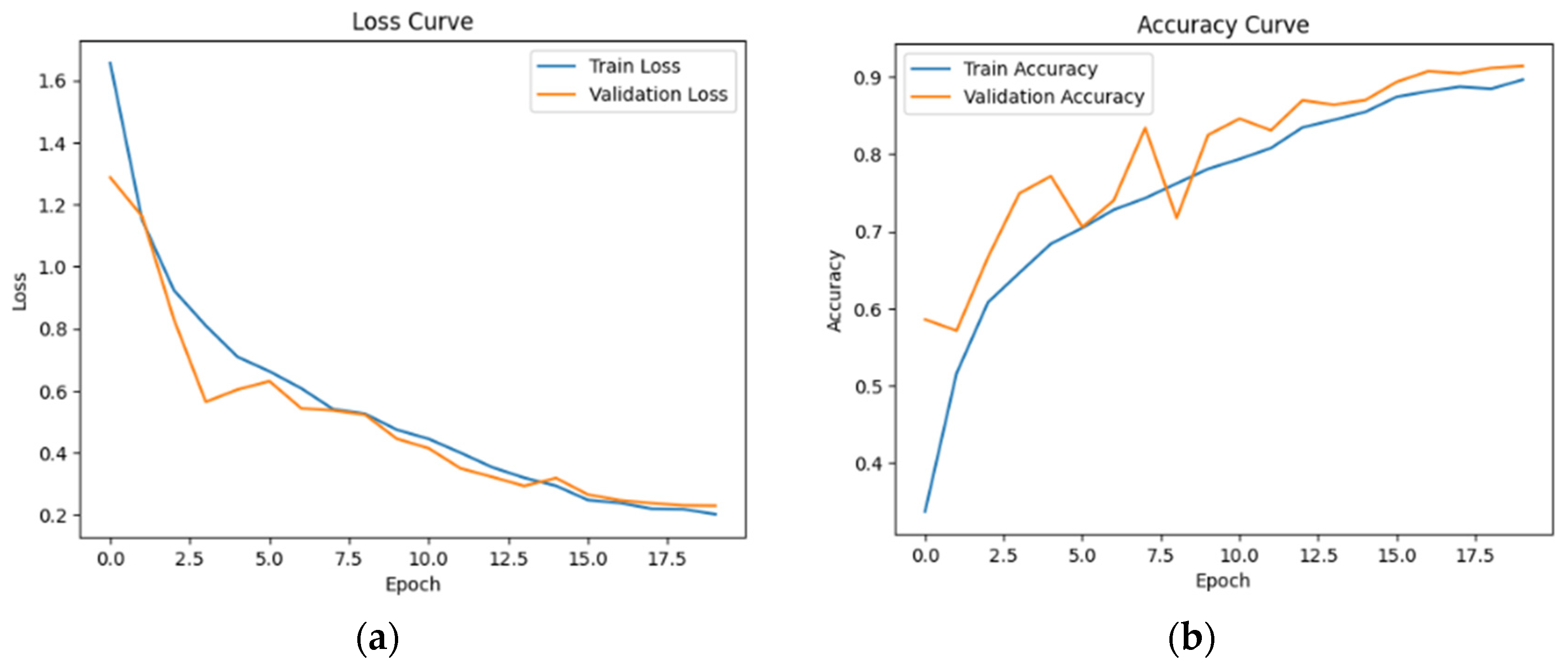
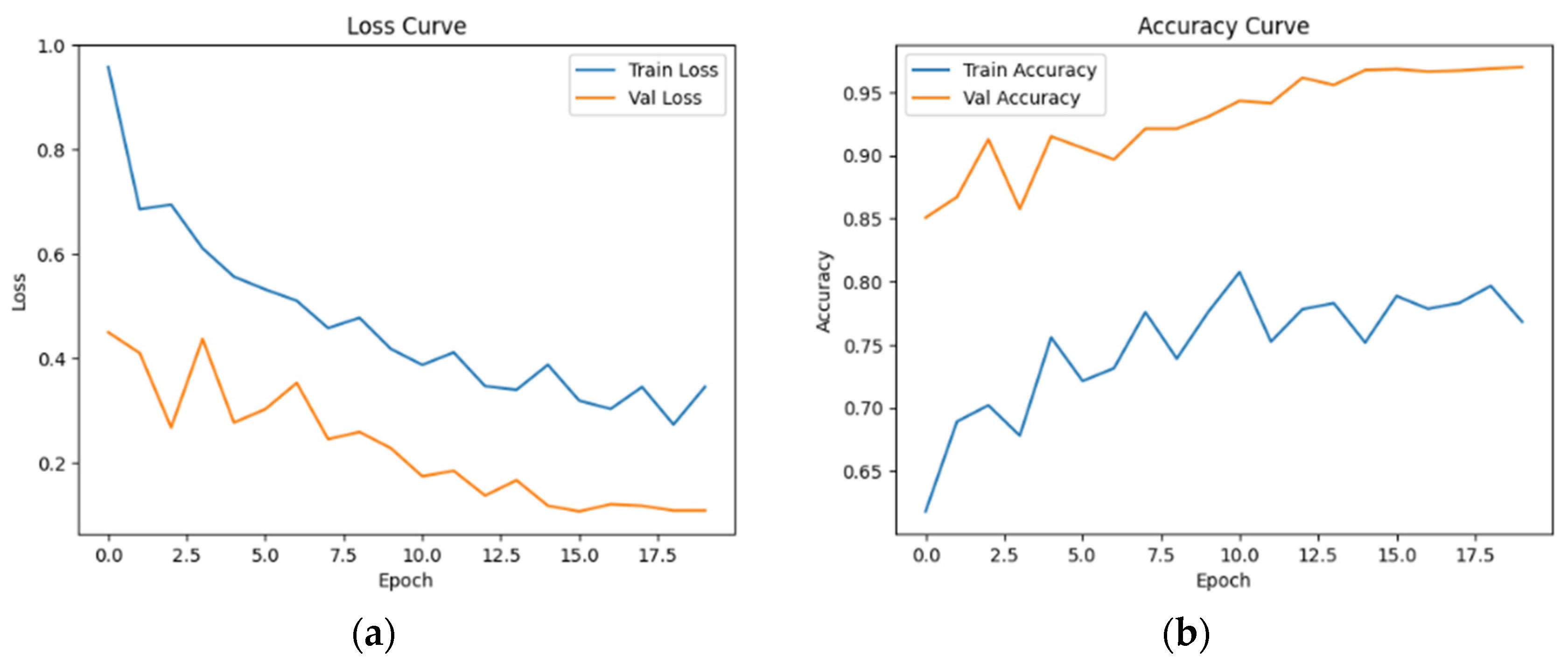
The Vision Transformer (ViT) showed higher results compared to all CNN models tested. After analyzing the training and verification curves, it was observed that ViT gave an accuracy of 96.9% with balancing, which was the highest performance obtained in all experiments.
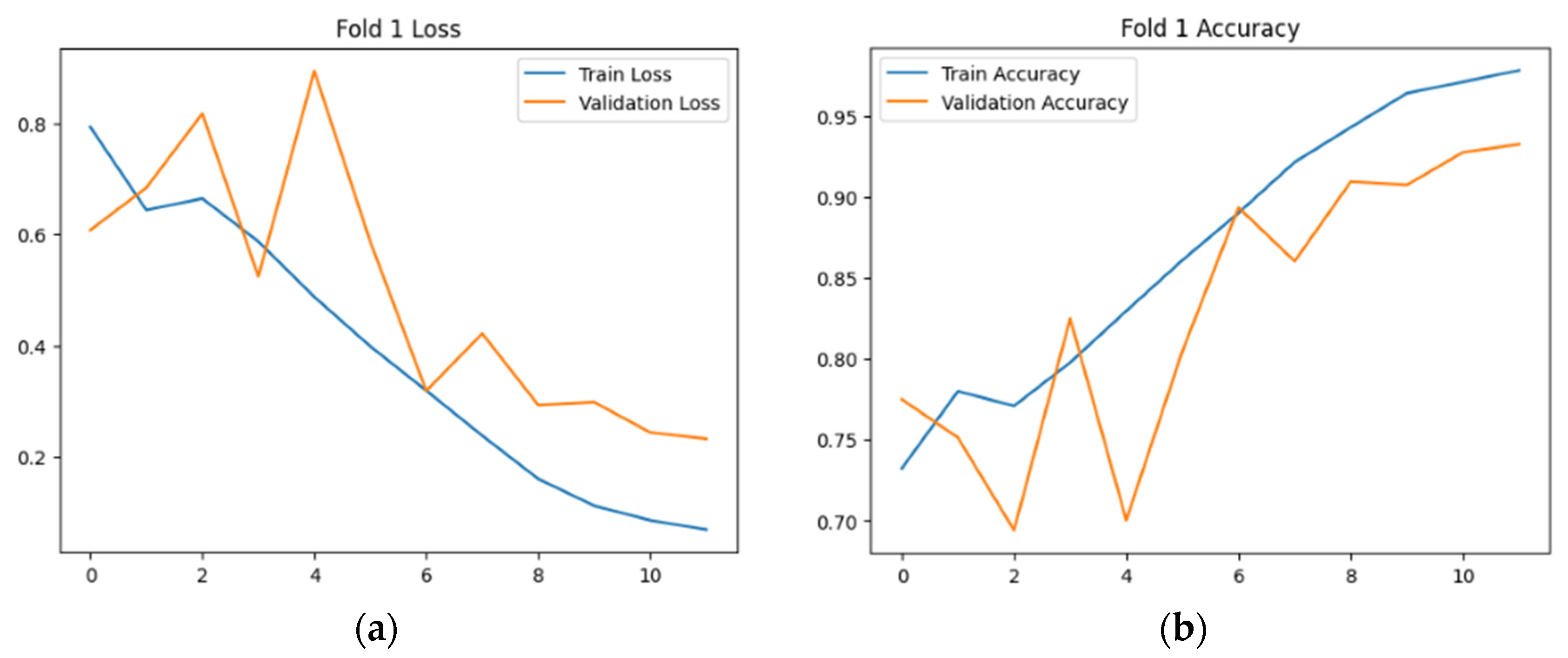
The model achieved high accuracy in Figure 11 and Figure 12, but its curves showed higher levels of volatility with greater differences between training and verification. This reflects that ViT has a greater ability to extract deep representations from DeepWeeds data, especially considering the class imbalance problem, where weighting helped improve performance. The accuracy curve of the ViT model shows remarkable stability after applying balancing using oversampling, as shown in Figure 12, where performance stabilizes quickly after a few training epochs without significant fluctuations, as shown in Figure 11 and Figure 13, indicating the model’s ability to generalize well.

4.2.3. ROC Curve Analysis

After analyzing the training and validation curves, the performance of the ViT model was examined using the ROC curve and measuring the area under the curve (AUC) for each class, as shown in Figure 14. The results showed that most classes achieved AUC values exceeding 0.95, demonstrating the model’s high ability to discriminate between samples.
The ROC curve showed an excellent distribution, in all categories approaching the optimal point (1, 1), which indicates high sensitivity (recall). The ROC curve also showed a sharp decline toward the upper left corner, reflecting a balance between correct detection rates and reduced false negatives. It achieved more stable performance compared to CNN models, which achieved AUC values below 0.90, while ViT maintained high and balanced performance even in rare categories.

4.2.4. Confusion Matrix Analysis

The performance of the ViT model was analyzed using a confusion matrix to evaluate how samples were classified across all categories. The results showed that the model successfully classified the vast majority of samples correctly, with errors mainly concentrated in categories with limited representation within the dataset. These were more prone to confusion with categories that were similar in visual appearance, which was reflected in a higher number of cross-errors between them. Compared to CNN models, ViT’s confusion matrix showed a more balanced distribution of errors, with a higher rate of correct predictions in rare categories. This reflects that ViT is able to leverage Class Weights to reduce model bias towards more represented classes, thereby promoting fairness among different classes.
A confusion matrix was used to analyze the model’s performance on the test data, as shown in Figure 15, which contains prediction images. This matrix shows a realistic evaluation of the ViT model’s performance on new, unprocessed, and unseen data, reflecting its ability to generalize.

4.3. Comparing Model Performance

4.3.1. Effect of Data Balancing Methods on Model Performance

Fine-tuning and balancing techniques were used in the experiments, enabling us to compare the performance of models using these techniques. The results of the experiments show that when using class weighting with strong augmentation, better results were achieved than when using the same settings with oversampling, as shown in the following Table 6. These results confirm the importance of data balancing in generalizing results and achieving high classification accuracy.
The performance of deep models was compared on the DeepWeeds dataset after standardizing the training settings. We conducted different experiments for each model to measure the stability of the results. As Table 6 shows, the proposed ViT-B/16 model with class weighting and oversampling achieved the best performance with an average accuracy of 96.9% compared to the traditional oversampling approach, which gave an accuracy of 94%, This confirms the effectiveness of class weighting in mitigating the bias of large classes. At the model level, the application of intelligent balancing using class weights instead of relying on traditional oversampling improved performance and reduced bias toward larger classes [37].

4.3.2. Compare Model Performance Using Data Balancing Methods

The proposed model ViT-B/16 was compared with several other models that were previously used in weed classification. While traditional models such as CNNs have been dominating this field for a long time, vision transformers have shown better indicators of accuracy and flexibility in dealing with large and complex data, making them a cutting-edge option at the present time. The proposed model can handle more diverse images in different environments using modern techniques such as self-learning; this result reflects the effectiveness of ViT in dealing with large and complex visual data, as can been seen in the following Table 7.
It is shown from the table that the ViT model significantly outperforms in accuracy compared to CNN models. It achieved 96.9% and outperforms other models, indicating its high efficiency in this field, which reflects the model’s ability to classify weeds with high accuracy in various environmental conditions. In terms of computational behavior on the reference GPU, ViT incurred higher per-epoch time and VRAM usage than EfficientNet-B0 and MobileNetV2, while CNNs trained faster and yielded lower-latency inference; this aligns with Table 2 parameterization and typical transformer memory footprints. As for flexibility in dealing with diverse data, unlike CNNs that may have difficulty dealing with complex and spatial patterns, the vision transformer model stands out thanks to the power of self-learning that allows it to handle diverse types of data (images, multispectral information, etc.) with greater flexibility, and the improvements in this model allowed a reduction in the computational burden compared to previous research. As for the ability to generalize in different environments, the current study demonstrated the model’s ability to operate in diverse environmental conditions while maintaining high accuracy, which represents a significant improvement over previous studies that suffered from decreased performance due to environmental changes (e.g., shade, lighting, and weather). It also achieves very high accuracy, and practical application in real environments via data augmentation techniques tested in diverse agricultural environments. It also improves performance efficiency, making the model applicable in a variety of scenarios.

4.3.3. Comparison with Studies Conducted on the Same Dataset

The proposed model ViT was compared with several other models that were previously used in weed classification. While traditional models such as CNNs have been dominating this field for a long time, achieving between 85% and 90% accuracy in classifying weeds. Although powerful, these models often have problems generalizing when the data are large and complex, or in cases of variable environmental conditions. Vision transformers have shown better indicators of accuracy and flexibility in dealing with large and complex data, making them a cutting-edge option at the present time [38], while RNNs have sometimes been used to classify weeds via sequential data (such as time or motion), they were unable to achieve high results in weed classification due to their poor performance in dealing with complex spatial patterns. While Multispectral image-assisted models [39]. Although these models have achieved good results in crop classification, ViT offers higher accuracy in recognizing complex patterns in diverse agricultural data [40]. The proposed model can handle more diverse images in different environments using modern techniques such as self-learning [41]. The vision transformer model stands out thanks to the power of self-learning that allows it to handle diverse types of data with greater flexibility, and the improvements in this model allowed for a reduction in the computational burden compared to previous research [11].
Compared to previous studies that used the DeepWeeds dataset, the results achieved fall within the range reported in those studies, with accuracy ranging between 90% and 95% in most studies. However, the results of the proposed model when using the augmentation and class weighting technique showed a significant improvement in terms of stability, accuracy, and high generalization ability compared to traditional oversampling. Therefore, it can be said that the strategy of assigning weights to underrepresented classes provides a better balance between high accuracy and reduced overfitting, the ViT model performed excellently in classifying weed species, achieving an accuracy of 96.9%. This proves that data enhancement is a key factor in improving the accuracy of classification models. It was also found that ViT models outperformed traditional convolutional networks in classification tasks, especially when using algorithm-level strategies such as class weighting or balanced tuning instead of relying on traditional oversampling. This demonstrates the effectiveness of transformer-based models in the image classification problem, especially when dealing with large and complex data as shown in Table 8.

4.4. Discussion

The experimental results show that lightweight convolutional models (ConvNeXt tiny, MobileNet, Regnetx_400mf, ShuffleNet, EfficientNet, and ResNet-18) are capable of achieving high performance in the weed classification task, which is consistent with previous studies that have confirmed the effectiveness of convolutional networks in agricultural computer vision applications. However, the performance of these models remains limited when attempting to distinguish between complex or very similar visual patterns, as they rely primarily on local filters that may not adequately capture long-range spatial relationships. In contrast, the ViT model showed clear superiority over all other models, achieving an accuracy of 96.9% compared to 94.6% for the best CNN model (EfficientNet B0). This superiority is attributed to the self-attention mechanism characteristic of ViT, which enables it to connect and analyze information distributed across the image in a comprehensive manner, enhancing its ability to distinguish between different types even in cases where the apparent features are similar. The results also confirm that incorporating preprocessing techniques such as class weighting and data augmentation solves the problem of class imbalance. Class weighting and augmentation techniques outperformed other techniques, contributing significantly to improving generalization and reducing the likelihood of overfitting. This is consistent with previous research on AI applications in precision agriculture, where data diversification and fair distribution across categories are critical factors for model success. Based on the above, ViT proves to be a promising option for weed classification applications, especially in scenarios that require high prediction accuracy and the processing of complex visual patterns and large, unbalanced data. However, the high computational cost of the ViT model compared to lightweight models may pose challenges when deploying it on resource-limited devices, necessitating the exploration of hybrid solutions or optimization techniques to reduce computational complexity without sacrificing performance.

4.5. Challenges and Limitations

Despite the model’s effective performance in classification, there were some challenges. Imbalance in distribution: It was observed that smaller categories (such as categories 3 and 4) were more prone to classification errors. The recall rate was good, but this may be due to poor data distribution among categories in the training set. Training duration: Training the ViT model requires a long time and significant computational resources due to the complexity of the architecture. This can be improved by using techniques such as smaller models or model transfer. Computational expense and scalability: Memory footprint and per-epoch time were higher for ViT than for lightweight CNNs on the reference GPU, which can limit batch sizes and slow iteration; mixed-precision training and gradient checkpointing are recommended. Practical deployment: Model size and inference latency should be considered for embedded devices/UAVs; lighter backbones or distilled/quantized ViTs may be preferred when on-board resources are constrained. Field applicability: Dataset-driven results should be complemented with prospective field trials under diverse soils/sky conditions to confirm stability under capture variations. Continuous improvement: The model can be further improved through model parameter optimization techniques. However, there are some limitations to the current approach, such as class imbalance; i.e., some weed species are underrepresented in the dataset, which may affect the model’s performance on those species. Future work could explore techniques such as oversampling or class weighting to address this issue. Training time: Being computationally intensive, the ViT model requires a significant amount of time and resources to train, especially when using large datasets. More efficient models or distributed training could alleviate this challenge.

5. Conclusions and Future Works

From an implementation perspective, inference speed, VRAM footprint, and model size should guide selection for edge platforms (e.g., UAVs/robots), where lighter CNNs or distilled/quantized ViTs can provide favorable trade-offs. This study addressed four aims: comparing ViT with competitive CNNs on DeepWeeds, analyzing data-imbalance strategies, providing initial interpretability via attention-based saliency inspection, and assessing consistency under location shift and capture perturbations using the dataset’s multi-site imagery. A framework was presented to solve the data imbalance problem, where the ViT model showed outstanding performance in classifying weeds using the DeepWeeds dataset. It achieved 96.9% accuracy and superior generalization ability, using class weighting and strong augmentation techniques, outperforming other models. These results can be used in smart farming applications to reduce weed damage and improve land management efficiency. The impact of imbalance on CNN and ViT will be demonstrated, as well as the sensitivity of traditional oversampling to hyper-adaptation, demonstrating the effectiveness of class weighting with strong augmentation as an alternative that achieves high accuracy.
In the future, the proposed model could be applied in precision agriculture to effectively identify weeds in agricultural land. It can also be integrated with artificial intelligence sensors such as agricultural robots to increase the efficiency of weed control operations, or unmanned aerial vehicles (UAVs), enhancing the model by using technologies to expand data or improve its distribution. Furthermore, technologies such as advanced neural networks, transfer learning, or hybrid models can be used to further improve results. Complementary techniques, such as the use of 8-bit integers used in the QWID model [45] can also be explored to reduce model size and inference time, which could reduce the area of resources used by up to 50% compared to traditional models. It is important to note that there may be a slight impact on classification accuracy, which must be carefully evaluated to ensure that performance is not significantly impacted. Future work could explore using scale models or modified deep learning techniques that work faster and more efficiently. Future research could explore techniques to further improve the model and address challenges such as incorporating Reinforcement Learning techniques to improve the model’s performance in unstable environments. This study opens up important future prospects for the development of hybrid models that combine the efficiency of convolutional models and the self-attention feature of transformers, as well as for exploring self-learning techniques to reduce the need for labeled data.
Author Contributions

Conceptualization, R.G. and S.M.; methodology, R.G. and S.M.; software, R.G. and S.M.; validation, R.G., S.M. and A.H.; formal analysis, R.G.; investigation, R.G.; resources, A.H.; data curation, R.G. and S.M.; writing—original draft preparation, R.G. and S.M.; writing—review and editing, R.G. and S.M.; visualization, R.G. and S.M.; supervision, A.H.; project administration, A.H.; funding acquisition, A.H. All authors have read and agreed to the published version of the manuscript.

Funding

This research received no external funding.

Data Availability Statement

Publicly available datasets were analyzed in this study. The data are from the DeepWeeds dataset and can be accessed at Kaggle: https://www.kaggle.com/datasets/imsparsh/deepweeds (accessed on 14 July 2025).

Conflicts of Interest

The authors declare no conflicts of interest.

References

  1. Wang, Y.; Zhang, S.; Dai, B.; Yang, S.; Song, H. Fine-grained weed recognition using Swin Transformer and two-stage transfer learning. Front. Plant Sci. 2023, 14, 1134932. [Google Scholar] [CrossRef] [PubMed]
  2. Hasan, A.S.M.M.; Sohel, F.; Diepeveen, D.; Laga, H.; Jones, M.G.K. A survey of deep learning techniques for weed detection from images. Comput. Electron. Agric. 2021, 184, 106067. [Google Scholar] [CrossRef]
  3. Monteiro, A.; Santos, S. Sustainable Approach to Weed Management: The Role of Precision Weed Management. Agronomy 2022, 12, 118. [Google Scholar] [CrossRef]
  4. Kamal, S.; Sharma, P.; Gupta, P.K.; Siddiqui, M.K.; Singh, A.; Dutt, A. DVTXAI: A novel deep vision transformer with an explainable AI-based framework and its application in agriculture. J. Supercomput. 2025, 81, 280. [Google Scholar] [CrossRef]
  5. Kamilaris, A.; Prenafeta-Boldú, F.X. Deep learning in agriculture: A survey. Comput. Electron. Agric. 2018, 147, 70–90. [Google Scholar] [CrossRef]
  6. Milioto, A.; Lottes, P.; Stachniss, C. Real-Time Semantic Segmentation of Crop and Weed for Precision Agriculture Robots Leveraging Background Knowledge in CNNs. In Proceedings of the 2018 IEEE International Conference on Robotics and Automation, Brisbane, QLD, Australia, 21–25 May 2018; pp. 2229–2235. [Google Scholar] [CrossRef]
  7. Qassim, H.M.; Hasan, W.Z.W.; Ramli, H.R.; Harith, H.H.; Mat, L.N.I.; Ismail, L.I. Proposed Fatigue Index for the Objective Detection of Muscle Fatigue Using Surface Electromyography and a Double-Step Binary Classifier. Sensors 2022, 22, 1900. [Google Scholar] [CrossRef]
  8. Dosovitskiy, A.; Beyer, L.; Kolesnikov, A.; Weissenborn, D.; Zhai, X.; Unterthiner, T.; Dehghani, M.; Minderer, M.; Herigold, G.; Gelly, S.; et al. An Image Is Worth 16 × 16 Words: Transformers for Image Recognition at Scale. In Proceedings of the ICLR 2021—9th International Conference on Learning Representations, Virtual, 3–7 May 2021. [Google Scholar]
  9. Khan, S.; Naseer, M.; Hayat, M.; Zamir, S.W.; Khan, F.S.; Shah, M. Transformers in Vision: A Survey. ACM Comput. Surv. 2022, 54, 1–41. [Google Scholar] [CrossRef]
  10. Radoglou-Grammatikis, P.; Sarigiannidis, P.; Lagkas, T.; Moscholios, I. A compilation of UAV applications for precision agriculture. Comput. Netw. 2020, 172, 107148. [Google Scholar] [CrossRef]
  11. Olsen, A.; Konovalov, D.A.; Philippa, B.; Ridd, P.; Wood, J.C.; Johns, J.; Bankds, W.; Girgenti, B.; Kenny, O.; Whinney, J.; et al. DeepWeeds: A Multiclass Weed Species Image Dataset for Deep Learning. Sci. Rep. 2019, 9, 2058. [Google Scholar] [CrossRef]
  12. Sunil, G.C.; Zhang, Y.; Howatt, K.; Schumacher, L.G.; Sun, X. Multi-Species Weed and Crop Classification Comparison Using Five Different Deep Learning Network Architectures. J. ASABE 2024, 67, 43–55. [Google Scholar] [CrossRef]
  13. Kussul, N.; Lavreniuk, M.; Skakun, S.; Shelestov, A. Deep Learning Classification of Land Cover and Crop Types Using Remote Sensing Data. IEEE Geosci. Remote Sens. Lett. 2017, 14, 778–782. [Google Scholar] [CrossRef]
  14. Liakos, K.G.; Busato, P.; Moshou, D.; Pearson, S.; Bochtis, D. Machine learning in agriculture: A review. Sensors 2018, 18, 2674. [Google Scholar] [CrossRef] [PubMed]
  15. Zhang, J. Weed Recognition Method based on Hybrid CNN-Transformer Model. Front. Comput. Intell. Syst. 2023, 4, 72–77. [Google Scholar] [CrossRef]
  16. SankarNath, S.; Rakshit, P. A Survey of Image Processing Techniques for Emphysema Detection. Int. J. Comput. Appl. 2015, 114, 7–13. [Google Scholar] [CrossRef]
  17. Qushtom, H.; Hasasneh, A.; Masri, S. Enhanced Wheat Disease Detection Using Deep Learning and Explainable AI Techniques. Comput. Mater. Contin. 2025, 84, 1379–1395. [Google Scholar] [CrossRef]
  18. Masri, S.; Hasasneh, A.; Tami, M.; Tadj, C. Exploring the Impact of Image-Based Audio Representations in Classification Tasks Using Vision Transformers and Explainable AI Techniques. Information 2024, 15, 751. [Google Scholar] [CrossRef]
  19. Hamuda, E.; Glavin, M.; Jones, E. A survey of image processing techniques for plant extraction and segmentation in the field. Comput. Electron. Agric. 2016, 125, 184–199. [Google Scholar] [CrossRef]
  20. Adewusi, A.O.; Asuzu, O.F.; Olorunsogo, T.; Iwuanyanwu, C.; Adaga, E.; Daraojimba, D.O. AI in precision agriculture: A review of technologies for sustainable farming practices. World J. Adv. Res. Rev. 2024, 21, 2276–2285. [Google Scholar] [CrossRef]
  21. Lochan, K.; Khan, A.; Elsayed, I.; Suthar, B.; Seneviratne, L.; Hussain, I. Advancements in Precision Spraying of Agricultural Robots: A Comprehensive Review. IEEE Access 2024, 12, 129447–129483. [Google Scholar] [CrossRef]
  22. Alirezazadeh, P.; Schirrmann, M.; Stolzenburg, F. A comparative analysis of deep learning methods for weed classification of high-resolution UAV images. J. Plant Dis. Prot. 2024, 131, 227–236. [Google Scholar] [CrossRef]
  23. Sishodia, R.P.; Ray, R.L.; Singh, S.K. Applications of remote sensing in precision agriculture: A review. Remote Sens. 2020, 12, 3136. [Google Scholar] [CrossRef]
  24. Tami, M.; Masri, S.; Hasasneh, A.; Tadj, C. Transformer-Based Approach to Pathology Diagnosis Using Audio Spectrogram. Information 2024, 15, 253. [Google Scholar] [CrossRef]
  25. Isinkaye, F.O.; Olusanya, M.O.; Akinyelu, A.A. A multi-class hybrid variational autoencoder and vision transformer model for enhanced plant disease identification. Intell. Syst. Appl. 2025, 26, 200490. [Google Scholar] [CrossRef]
  26. Simonyan, K.; Zisserman, A. Very deep convolutional networks for large-scale image recognition. In Proceedings of the 3rd International Conference on Learning Representations, ICLR 2015—Conference Track Proceedings, San Diego, CA, USA, 7–9 May 2015; pp. 1–14. [Google Scholar]
  27. Maurício, J.; Domingues, I.; Bernardino, J. Comparing Vision Transformers and Convolutional Neural Networks for Image Classification: A Literature Review. Appl. Sci. 2023, 13, 5521. [Google Scholar] [CrossRef]
  28. Arifin, K.N.; Rupa, S.A.; Anwar, M.M.; Jahan, I. Lemon and Orange Disease Classification using CNN-Extracted Features and Machine Learning Classifier. In Proceedings of the 3rd International Conference on Computing Advancements, Dhaka, Bangladesh, 17–18 October 2024; pp. 154–161. [Google Scholar] [CrossRef]
  29. Vaghefi, S.A.; Ibrahim, M.F.; Zaman, M.H.M.; Mustafa, M.M.; Mustaza, S.M.; Zulkifley, M.A. Optimized Weed Image Classification via Parallel Convolutional Neural Networks Integrating an Excess Green Index Channel. Int. J. Electr. Comput. Eng. Syst. 2025, 16, 205–216. [Google Scholar] [CrossRef]
  30. Alzubaidi, L.; Zhang, J.; Humaidi, A.J.; Al-Dujaili, A.; Duan, Y.; Al-Shamma, O.; Santamaría, J.; Fadhei, M.A.; Al-Amidie, M.; Farhan, L. Review of deep learning: Concepts, CNN architectures, challenges, applications, future directions. J. Big Data 2021, 8, 53. [Google Scholar] [CrossRef] [PubMed]
  31. Pan, X.; Ge, C.; Lu, R.; Song, S.; Chen, G.; Huang, Z.; Huang, G. On the Integration of Self-Attention and Convolution. In Proceedings of the IEEE Conference on Computer Vision and Pattern Recognition, New Orleans, LA, USA, 18–24 June 2022; pp. 805–815. [Google Scholar] [CrossRef]
  32. Furfari Tony, F.A. The Transformer. IEEE Ind. Appl. Mag. 2002, 8, 8–15. [Google Scholar] [CrossRef]
  33. Cawley, G.C.; Talbot, N.L.C. On over-fitting in model selection and subsequent selection bias in performance evaluation. J. Mach. Learn. Res. 2010, 11, 2079–2107. [Google Scholar]
  34. Tsao, C.C. Chapter 20. In Shanghai Bride; Hong Kong University Press: Hong Kong, 2025; Volume 197, pp. 152–156. [Google Scholar] [CrossRef]
  35. Xu, Z.; Liu, R.; Yang, S.; Chai, Z.; Yuan, C. Learning Imbalanced Data with Vision Transformers. In Proceedings of the IEEE Conference on Computer Vision and Pattern Recognition, Vancouver, BC, Canada, 17–24 June 2023; pp. 15793–15803. [Google Scholar] [CrossRef]
  36. Mulay, V.M.; Rao, M.; Kumar, K.V. Ensemble based Deep Learning Models for Crop and Weed Differentiation. Meas. Digit. 2025, 2–3, 100009. [Google Scholar] [CrossRef]
  37. Rawat, S.S.; Mishra, A.K. Review of Methods for Handling Class Imbalance in Classification Problems. Lect. Notes Electr. Eng. 2024, 1146, 3–14. [Google Scholar] [CrossRef]
  38. Takahashi, S.; Sakaguchi, Y.; Kouno, N.; Takasawa, K.; Ishizu, K.; Akagi, Y.; Aoyama, R.; Teraya, N.; Bolatkan, A.; Shinkai, N.; et al. Comparison of Vision Transformers and Convolutional Neural Networks in Medical Image Analysis: A Systematic Review. J. Med. Syst. 2024, 48, 84. [Google Scholar] [CrossRef]
  39. Sarmadi, A.; Razavi, Z.S.; van Wijnen, A.J.; Soltani, M. Comparative analysis of vision transformers and convolutional neural networks in osteoporosis detection from X-ray images. Sci. Rep. 2024, 14, 18007. [Google Scholar] [CrossRef]
  40. Lee, C.P.; Lim, K.M.; Song, Y.X.; Alqahtani, A. Plant-CNN-ViT: Plant Classification with Ensemble of Convolutional Neural Networks and Vision Transformer. Plants 2023, 12, 2642. [Google Scholar] [CrossRef] [PubMed]
  41. Ferreira, B.P.; Moreira, P.H.C.; Silva, L.H.F.P.; Mari, J.F. Evaluating Deep Learning Models for Effective Weed Classification in Agricultural Images. Rev. Informática Teórica Apl. 2025, 32, 265–272. [Google Scholar] [CrossRef]
  42. Ali, H.; Shifa, N.; Benlamri, R.; Farooque, A.A.; Yaqub, R. A fine tuned EfficientNet-B0 convolutional neural network for accurate and efficient classification of apple leaf diseases. Sci. Rep. 2025, 15, 25732. [Google Scholar] [CrossRef] [PubMed]
  43. Zi, J.; Hu, W.; Fan, G.; Chen, F.; Chen, Y. SFL-MobileNetV3: A lightweight network for weed recognition in tropical cassava fields in China. Expert Syst. Appl. 2025, 277, 127196. [Google Scholar] [CrossRef]
  44. Rozendo, G.B.; Roberto, G.F.; do Nascimento, M.Z.; Alves Neves, L.; Lumini, A. Weeds classification with deep learning: An investigation using CNN, Vision Transformers, Pyramid Vision Transformers, and ensemble strategy. In Progress in Pattern Recognition, Image Analysis, Computer Vision, and Applications; Springer: Cham, Switzerland, 2025. [Google Scholar]
  45. Rathore, P.S. QWID: Quantized Weed Identification Deep neural network. In Proceedings of the 2024 IEEE 31st International Conference on High Performance Computing, Data and Analytics Workshop (HiPCW), Bangalore, India, 18–21 December 2024; pp. 223–224. [Google Scholar] [CrossRef]
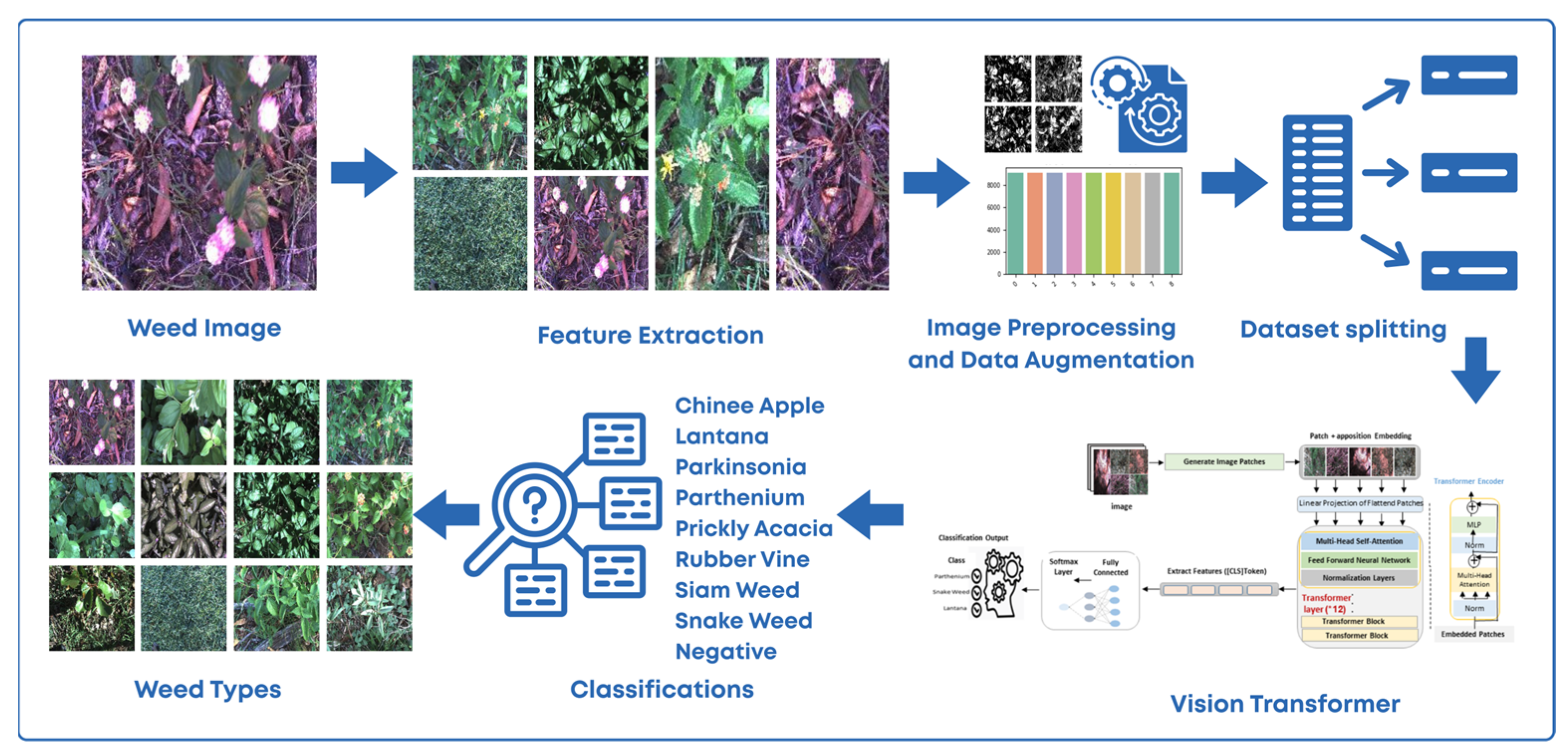
Figure 1. WeedNet-ViT overview. Following the arrows of the graph: sample DeepWeeds images; feature-tile montage, augmentation previews, and split/distribution graphic; Vision Transformer (ViT) module and prediction panel; class exemplars (“Type of Weed”) with example labels (Parthenium, Snake Weed, Lantana).
Geographies 05 00064 g001
Figure 2. A sample from a herb dataset consisting of nine classes (0–8). Three random images represent each class. The numbers above the images (0–8) represent the class IDs.
Geographies 05 00064 g002
Figure 3. The dataset shows over sampling techniques in (a) weeds before balancing and in (b) after balancing.
Geographies 05 00064 g003
Figure 4. The dataset shows class weighting techniques in (a) weeds before balancing and in (b) after balancing.
Geographies 05 00064 g004
Figure 5. The proposed model structure based on CNN.
Geographies 05 00064 g005
Figure 6. Architecture of the proposed vision transformer. The asterisk () denotes that the Transformer layer is repeated 12 times *.
Geographies 05 00064 g006
Figure 7. Training/validation accuracy for the best CNN baseline: (a) before balancing, (b) oversampling, (c) class weighting; weighting improves validation stability.
Geographies 05 00064 g007
Figure 8. Loss curves for the superior CNN baseline: (a) before balancing, (b) oversampling, (c) class weighting; loss stabilizes with weighting.
Geographies 05 00064 g008
Figure 9. ROC curves for the superior CNN baseline: (a) before balancing, (b) oversampling, (c) class weighting; AUC remains high across settings.
Geographies 05 00064 g009
Figure 10. Confusion Matrices to the superior CNN model: (a) Before Balancing (b) Oversampling techniques and (c) Class weighting techniques.
Geographies 05 00064 g010
Figure 11. Accuracy and loss curves before balancing: (a) loss curve; (b) accuracy curve.
Geographies 05 00064 g011
Figure 12. Accuracy and loss curves with oversampling: (a) loss curve; (b) accuracy curve.
Geographies 05 00064 g012
Figure 13. Accuracy and loss curves with class weighting: (a) loss curve; (b) accuracy curve.
Geographies 05 00064 g013
Figure 14. Accuracy and Loss Curves with balancing Class Weighting techniques: (a) Before Balancing, (b) Oversampling techniques and (c) Class weighting techniques.
Geographies 05 00064 g014
Figure 15. Confusion Matrix ViT Model: (a) Before Balancing, (b) Oversampling techniques and (c) Class weighting techniques.
Geographies 05 00064 g015
Table 1. Distribution of the 9 sample categories.
ClassesNumber of Images
Chinee Apple1125
Lantana1064
Parkinsonia1031
Parthenium1022
Prickly Acacia1062
Rubber Vine1009
Siam Weed1074
Snake Weed1016
Negative9106
Total17,509
Table 2. Specifications of the ViT model.
FeatureSpecification
Model NameViT-Base Patch16 224
Patch Size16 × 16 pixels
Image Size224 × 224 pixels
Hidden Size768
Number of Layers12 transformer encoder layers
MLP Size1009
Number of Attention Heads3072
Total Parameters85,805,577
Model NameViT-Base Patch16 224
Table 3. Hyperparameters of proposed Vision Transformer.
HyperparametersValue
Learning Rate0.001
Initial LR0.0001
Weight Decay0.0001
Num Epochs10
Max Epoch30
Batch Size32
Raw IMG Size(256, 256)
IMG Size(224, 224)
OptimizerAdamW
SchedulerOneCycleLR
Table 4. CNN model training and validation results.
CNN ModelsBefore BalancingOversamplingClass Weight
EfficientNet B098.2%92.3%94.6%
ConvNeXt-Tiny96.6%91.1%93.2%
MobileNetV294.5%89.4%91.8%
RegNet_X_400MF94.9%91.7%93.9%
ResNet1893.1%87.4%91.1%
ShuffleNetV291.488.5%91.4%
Table 5. Classification Report.
CategoryPrecisionRecallF1-ScoreSupport
Chinee Apple0.950.960.95169
Lantana0.980.980.98160
Parkinsonia0.980.990.99155
Parthenium0.970.980.97153
Prickly Acacia0.940.970.96160
Rubber Vine0.950.970.96151
Siam Weed0.980.980.98161
Snake Weed0.950.930.94152
Negative0.980.980.981366
Table 6. Effect of data-balancing strategies on ViT: macro-F1 and accuracy under no balancing, class weighting (PyTorch class weights), and oversampling.
ModelPreparationMacro F1 (%)Accuracy (%)Notes
ViTNo balancing97%99.9%Weak generalization
ViTClass weighting97%96.9%Significant improvement in rare categories
ViTOversampling91%94%Increased risk of overfitting for rare classes
Table 7. Comparing the ViT model with other models.
ModelPrecision %Recall %F1-Score %Accuracy %
ViT95969796.9
ResNet1888909192.1
EfficentNetV294949494.5
Regnetx_400mf94949494.9
MobileNet V292949292.8
EfficentNetB095969595.6
ConvNeXt Tiny94959394.2
ShuffleNet V292929192.4
ResNet5082918788.4
Table 8. Comparison with Prior Studies on the DeepWeeds Dataset (Accuracy %).
ModelStudiesAccuracy %Proposed Models Accuracy %
ViT[11]98.5096.71
ConvNeXt[29]99.099.40
ResNet50[11]95.7096.20
EfficientNet-B0[42]77.1096.63
MobileNetV3[43]94.3494.51
DenseNet-201[44]94.6794.85
ViT[15]96.8096.90
Disclaimer/Publisher’s Note: The statements, opinions and data contained in all publications are solely those of the individual author(s) and contributor(s) and not of MDPI and/or the editor(s). MDPI and/or the editor(s) disclaim responsibility for any injury to people or property resulting from any ideas, methods, instructions or products referred to in the content.